Lecture 3: Discrete Time Stability and MIMO Systems
1 Discrete-time Systems 2.0
1.1 Discrete-time Systems Stability
We want to investigate the stability conditions for the discrete-time system given as x[k+ 1] =Adx[k] +Bdu[k]
y[k] =Cdx[k] +Ddu[k], x[0] =x0. (1.1) As usual, we want to find conditions for wich the state x[k] does not diverge. The free evolution (free means without input) can be written as
x[k+ 1] =Adx[k]. (1.2)
Starting from the initial state, one can write x[1] = Adx0 x[2] = A2dx0
...
x[k] =Akdx0.
(1.3)
In order to analyze the convergence of this result, let’s assume that Ad ∈ Rn×n is diago- nalizable and let’s rewrite Ad with the help of its diagonal form:
x[k] =Akdx0
= T DT−1k
x0
= T D T−1T
| {z }
I
DT−1. . . T DT−1
!
=T DkT−1x0.
(1.4)
where D is the matrix containing the eigenvalues of Ad and T is the matrix containing the relative eigenvectors. One can rewrite this using the modal decomposition as
T DkT−1x0 =
n
X
i=1
αiλkivi, (1.5)
where vi are the eigenvectors relative to the eigenvalues λi and αi = T−1x0 some coef- ficients depending on the initial condition x0. Considering any possible eigenvalue, i.e.
λi =ρiejφi, one can write
T DkT−1x0 =
n
X
i=1
αiρkiejφikvi. (1.6)
It holds
|λi|=ρki|ejφik|
=ρki. (1.7)
This helps us defining the following cases:
• |λi| <1 ∀i= 1, . . . , n: the free evolution converges to 0 and the system is asymp- totically stable.
• |λi| ≤ 1∀i= 1, . . . , nand eigenvalues with unit modulus have equal geometric and algebraic multiplicity: the free evolution converges (but not to 0) and the system is marginally stable orstable.
• ∃i s.t. |λi|>1: the free evolution diverges and the system is unstable.
Remark. The same analysis can be performed for non diagonalizable matrices Ad. The same conditions can be derived, with the help of the Jordan diagonal form of Ad.
Example 1. You are given the dynamics x[k+ 1] =
0 0 1 12
| {z }
Ad
x[k], x[0] = x10
x20
. (1.8)
SinceAd is a lower diagonal matrix, its eigenvalues lie in the diagonal, i.e. λ1 = 0, λ2 = 12. Since both eigenvalues satisfy |λi|<1, the system is asymptotically stable.
1.2 Discrete Time Controller Synthesis
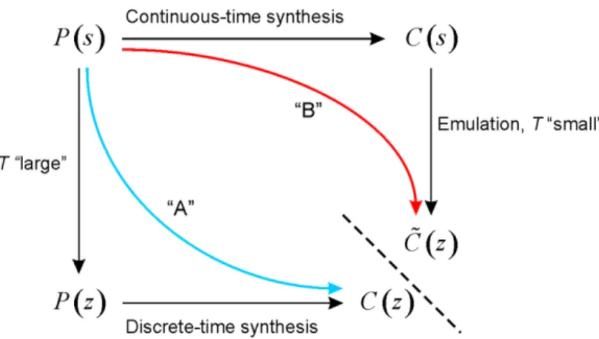
As you learned in class, there are two ways to discretize systems. The scheme in Figure 1 resumes them.
Figure 1: Emulation and Discrete time controller synthesis.
1.2.1 Emulation
In the previous chapter, we learned how to emulate a system. Let’s define the recipe for such a procedure: Given a continous-time plant P(s):
1. Design a continuous-time controller for the continuous-time plant.
2. Choose a sampling rate that is at least twice (ten times in practice) the crossover frequency.
3. If required, design an anti aliasing filter (AAF) to remove high frequency components of the continuous signal that is going to be sampled.
4. Modify your controller to take into accout the phase lag introduced by the dis- cretization (up to a sampling period delay) and the AAF.
5. Discretize the controller (e.g. use the Tustin method for best accuracy).
6. Check open loop stability. If the system is unstable, change the emulation method, choose a faster sampling rate, or increase margin of phase.
7. Implement the controller.
1.2.2 Discrete-Time Synthesis
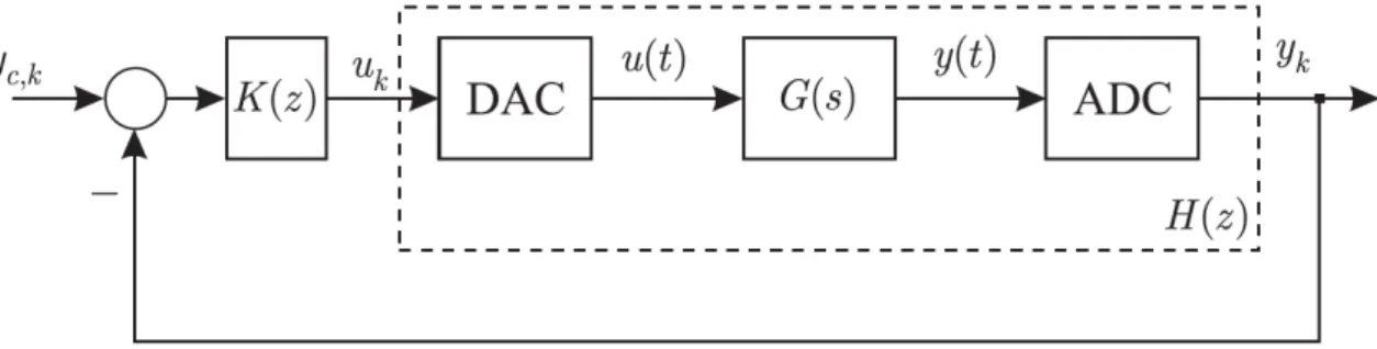
In this chapter we learn how to perform discrete time controller synthesis (also called direct synthesis). The general situation is the following: a control loop is given as in Figure 2. The continuous time transfer function G(s) is given.
Figure 2: Discrete-time control loop.
We want to compute the equivalent discrete-time transfer function H(z). The loop is composed of a Digital-to-Analog Converter (DAC), the continuous-time transfer function G(s) and of an Analog to Digital Converter (ADC). We aim reaching a structure that looks like the one in Figure 3.
The first thing to do, is to consider an input to analyze. The usual choice for this type of analysis is a unit-stepof the form
u(kT) = {. . . ,0,1,1, . . .}. (1.9) Since the z−Transform is defined as
X(z) =
∞
X
n=0
x(n)·z−n (1.10)
K(z) H(z)
yr ε(z) U(z) Y(z)
n= 0
−
Figure 3: Discrete Syhtesis.
one gets for u
U(z) = 1 +z−1+z−2+z−3+. . .+z−n. (1.11) This sum can be written as (see geometric series)
U(z) = 1
1−z−1. (1.12)
For U(z) to be defined, this sum must converge. This can be verified by exploring the properties of the geometric series.
Remark. Recall: sum of geometric series Let Sn denote the sum over the first n elements of a geometric series:
Sn =U0+U0·a+U0·a2+. . .+U0·an−1
=U0·(1 +a+a2+. . .+an−1). (1.13) Then
a·Sn=U0·(a+a2+a3+. . .+an) (1.14) and
Sn−a·Sn=U0·(1−an), (1.15) which leads to
Sn =U0· 1−an
1−a . (1.16)
From here, it can be shown that the limit for n going to infinity convergenges if and only if the absolute value of a is smaller than one, i.e.
n→∞lim Sn=U0· 1
1−a, iff |a|<1. (1.17) Therefore the limiting case |a|= 1 =:ris called radius of convergence. The according convergence criterion is|a|< r.
H(z) contains the converters: at first, we have the digital -to-analog converter. The Laplace-Transform of the unit-step reads generally
1
s. (1.18)
Hence, the transfer function before the analog-to-digital converter reads G(s)
s . (1.19)
In order to consider the analog-to-digital converter, we have to apply the inverse Laplace transfrom to get
y(t) = L−1
G(s) s
. (1.20)
Through a z− transform one can now get Y(z). It holds Y(z) = Z(y(kT))
=Z
L−1
G(s) s
. (1.21)
The transfer function is then given as
H(z) = Y(z)
U(z). (1.22)
Example 2. A continuous-time system with the following transfer function is considered:
G(s) = 9
s+ 3. (1.23)
(a) Calculate the equivalent discrete-time transfer function H(z). The latter is com- posed of a Digital-to-Analog Converter (DAC), the continuous-time transfer function G(s) and an Analog-to-Digital Converter (ADC). Both converters, i.e. the DAC and ADC, have a sampling time Ts= 1s.
(b) Calculate the static error if a proportional controller K(z) = kp is used and the reference input yc,k is a step signal.
Hint: Heavyside with amplitude equal to 1.
Solution.
(a) Rather than taking into account all the individual elements which make up the continuous-time part of the system (DAC, plant, ADC), in a first step, these el- ements are lumped together and are represented by the discrete-time description H(z). In this case, the discrete-time output of the system is given by
Y(z) =H(z)·U(z), (1.24)
whereU(z) is thez−transform of the discrete input uk given to the system. There- fore, the discrete-time representation of the plant is given by the ratio of the output to the input
H(z) = Y(z)
U(z). (1.25)
For the sake of convenience,uk is chosen to be the discrete-time Heaviside function (uk[k] = 1, k≥0
0, else. (1.26)
This input function needs to be z−transformed. Recall the definition of the z- transform
X(z) =
∞
X
n=0
x(n)·z−n. (1.27)
and applying it to the above equation, with the input uk gives (uk[k] = 1 fork ≥0) U(z) =X(uk)
=
∞
X
k=0
z−k
=
∞
X
k=0
(z−1)k.
(1.28)
For U(z) to be defined, this sum must converge. Recalling the properties of geo- metric series one can see
U(z) = 1
a−z−1, (1.29)
as long as the convergence criterion is satisfied, i.e. as long as |z−1| < 1 or better
|z| > 1 (a = 1). This signal is then transformed to continuous time using a zero- order hold DAC. The output of this transformation is again a Heaviside function uh(t). Since the signal is now in continuous time, the Laplace transform is used to for the analysis. The Laplace transform of the step function is well known to be
L(uh(t))(s) = 1
s =U(s). (1.30)
The plant output in continuous time is given by Y(s) = G(s)·U(s)
= G(s)
s . . (1.31)
After the plant G(s), the signal is sampled and transformed into discrete time once more. Therefore, thez−transform of the output has to be calculated. However, the signal Y(s) cannot be transformed directly, since it is expressed in the frequency domain. Thus, first, it has to be transformed back into the time domain (i.e. into y(t)) using the inverse Laplace transform, where it is then sampled every t=k·T. The resulting series of samples{y[k]} is then transformed back into thez−domain, i.e.
Y(z) =X
{L−1
G(s) s
(kT)}
. (1.32)
To find the inverse Laplace transform of the output, its frequency domain represen- tation is decomposed into a sum of simpler functions
G(s)
s = 9
s·(s+ 3)
= α s + β
s+ 3
= s·(α+β) + 3·α s·(s+ 3) .
(1.33)
The comparison of the numerators yields
α= 3, β =−3.
and thus
G(s) s = 3
s − 3 s+ 3
= 3· 1
s − 1 s+ 3
.
(1.34)
Now the terms can be individually transformed with the result L−1
G(s) s
= 3· 1−e−3t
·uh(t)
=y(t).
(1.35)
The z−transform of the output sampled at discrete time istants y(kT) is given by X({y(kT)}) = 3·
" ∞ X
k=0
z−k−
∞
X
k=0
e−3kT ·z−k
#
= 3·
" ∞ X
k=0
z−1k−
∞
X
k=0
(e−3T ·z−1)k
#
=Y(z).
(1.36)
From above, the two necessary convergence criteria are known:
|z−1|<1⇒ |z|>1
|e−3T ·z−1| ⇒ |z|>|e−3T|. (1.37) Using the above equations the output transfrom converges to (given that the two convergence criteria are satisfied)
Y(z) = 3·
1
1−z−1 − 1 1−e−3T ·z−1
. (1.38)
Finally, the target transfer function H(z) is given by H(z) = Y(z)
U(z)
= (1−z−1)·Y(z)
= 3·
1− 1−z−1 1−e−3T ·z−1
= 3· (1−e−3T)·z−1 1−e−3T ·z−1 .
(1.39)
(b) From the signal flow diagram, it can be seen that the error ε(z) is composed of ε(z) =Yc(z)−Y(z)
=Yc(z)−H(z)·K(z)·ε(z)
= Yc(z) 1 +kp ·H(z).
(1.40)
The input yc(t) is a discrete step signal, for which the z-transform was calculated in (a):
Yc(z) = 1
1 +z−1. (1.41)
Therefore, the error signal reads ε(z) =
1 1+z−1
1 + 3·kp· (1−e1−e−3T−3T)·z·z−1−1
. (1.42)
To calculate the steady-state error, i.e. the error after infinite time, the discrete-time final value theorem1 is used:
t→∞lim ε(t) = lim
z→1(1−z−1)·ε(z), (1.43) but as z goes to 1, so doesz−1 and thereforem 1 is substituted for each z−1 in ε(z) and the stati error becomes
ε∞= 1
1 + 3·kp. (1.44)
Note that the error does not completely vanish but can be made smaller by increasing kp. This is the same behaviour which would have been expected from a purely proportional controller in continuous time. To drive the static error to zero, a discrete-time integrator of the form T 1
i·(1−z−1) would be necessary.
1limt→∞ε(t) = lims→0s·ε(s)
2 MIMO Systems
MIMO systems are systems with multiple inputs and multiple outputs. In this chapter we will introduce some analytical tools.
2.1 System Description
2.1.1 State Space Descriprion
The state-space description of a MIMO system is very similar to the one of a SISO system.
For a linear, time invariant MIMO system with m input signals and p output signals, it holds
˙
x(t) =A·x(t) +B·u(t), x(t)∈Rn, u(t)∈Rm y(t) =C·x(t) +D·u(t), y(t)∈Rp
(2.1) where
x(t)∈Rn×1, u(t)∈Rm×1, y(t)∈Rp×1, A∈Rn×n, B ∈Rn×m, C ∈Rp×n, D ∈Rp×m. (2.2) Remark. The dimensions of the matrices A, B, C, D are very important and they are a key concept to understand problems.
The big difference from SISO systems is that u(t) and y(t) are here vectors and not scalars anymore. For this reason B, C, D are now matrices.
2.1.2 Transfer Function
One can compute the transfer function of a MIMO system with the well known formula P(s) =C·(s·I−A)−1·B+D. (2.3) This is no more a scalar, but a p×m-matrix. The elements of that matrix are rational functions. Mathematically:
P(s) =
P11(s) · · · P1m(s) ... . .. ... Pp1(s) · · · Ppm(s)
, Pij(s) = bij(s)
aij(s). (2.4) Here Pij(s) is the transfer function from the j-th input to the i-th output.
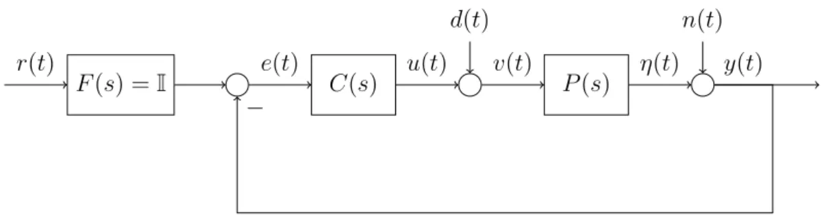
Remark. In the SISO case, the only matrix we had to care about was A. Since for the MIMO caseB,C,Dare matrices, one has to pay attention to a fundamental mathematical property: the matrix multiplication is not commutative (i.e. A·B 6=B·A). Since now P(s) and C(s) are matrices, considering Figure 4, it holds
LO(s) =P(s)·C(s)6=C(s)·P(s) = LI(s), (2.5) where LO(s) is the outer loop transfer function andLI(s) is the inner loop transfer func- tion. Moreover, one can no more define the complementary sensitivity and the sensitivity as
T(s) = L(s)
1 +L(s), S(s) = 1
1 +L(s). (2.6)
because no matrix division is defined. There are however similar expressions to describe those transfer functions:
F(s) =I C(s)
d(t)
P(s)
n(t)
r(t) e(t) u(t) v(t) η(t) y(t)
−
Figure 4: Standard feedback control system structure.
Output Sensitivity Functions Referring to Figure 5, one can write
Y(s) = N(s) +η(s)
=N(s) +P(s)V(s)
=N(s) +P(s) (D(s) +U(s))
=N(s) +P(s) (D(s) +C(s)E(s))
=N(s) +P(s) (D(s) +C(s)(R(s)−Y(s))),
(2.7)
from which follows
(I+P(s)C(s))Y(s) =N(s) +P(s)D(s) +P(s)C(s)R(s)
Y(s) = (I+P(s)C(s))−1(N(s) +P(s)D(s) +P(s)C(s)R(s)). (2.8) It follows
• Output sensitivity function (n→y)
SO(s) = (I+LO(s))−1. (2.9)
• Output complementary sensitivity function (r →y)
TO(s) = (I+LO(s))−1LO(s). (2.10) Input Sensitivity Functions
Referring to Figure 5, one can write U(s) = C(s)E(s)
=C(s) (R(s)−Y(s))
=C(s)R(s)−C(s) (N(s) +η(s))
=C(s)R(s)−C(s)N(s)−C(s)P(s)V(s)
=C(s)R(s)−C(s)N(s)−C(s)P(s) (D(s) +U(s)),
(2.11)
from which it follows
(I+C(s)P(s))U(s) =C(s)R(s)−C(s)N(s)−C(s)P(s)D(s)
−U(s) = (I+C(s)P(s))−1(−C(s)R(s) +C(s)N(s) +C(s)P(s)D(s)). (2.12) It follows
• Input sensitivity function (d→v)
SI(s) = (I+LI(s))−1. (2.13)
• Input complementary sensitivity function (d→ −u)
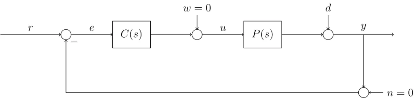
TI(s) = (I+LI(s))−1LI(s). (2.14) Example 3. In order to understand how to work with these matrices, let’s analyze the following problem. We start from the standard control system’s structure (see Figure 5).
To keep things general, let’s say the plant P(s)∈Cp×m and the controller C(s)∈ Cm×p. The reference r ∈ Rp, the input u ∈ Rm and the disturbance d ∈ Rp. The output Y(s) can as always be written as
Y(s) = T(s)·R(s) +S(s)·D(s). (2.15) where T(s) is the transfer function of the complementary sensitivity and S(s) is the transfer function of the sensitivity.
C(s)
w= 0
P(s)
d
r e u y
n= 0
−
Figure 5: Standard feedback control system structure.
Starting from the error E(s)
If one wants to determine the matrices of those transfer functions, one can start writing (by paying attention to the direction of multiplications) with respect to E(s)
E(s) =R(s)−P(s)·C(s)·E(s)−D(s),
Y(s) =P(s)·C(s)·E(s) +D(s). (2.16) This gives in the first place
E(s) = (I+P(s)·C(s))−1·(R(s)−D(s)). (2.17) Inserting and writing the functions as F(s) = F for simplicity, one gets
Y =P ·C·E+D
=P ·C·(I+P ·C)−1·(R−D) +D
=P ·C·(I+P ·C)−1·R−P ·C(I+P ·C)−1·D+ (I+P ·C) (I+P ·C)−1
| {z }
I
·D
=P ·C·(I+P ·C)−1·R+ (I+P ·C−P ·C)·(I+P ·C)−1·D
=P ·C·(I+P ·C)−1·R+ (I+P ·C)−1·D.
(2.18)
Recalling the general equation (2.15) one gets the two transfer functions:
T1(s) = P(s)·C(s)·(I+P(s)·C(s))−1,
S1(s) = (I+P(s)·C(s))−1. (2.19) Starting from the input U(s)
If one starts with respect to U(s), one gets
U(s) =C(s)·(R(s)−D(s))−C(s)·P(s)·U(s),
Y(s) =P(s)·U(s) +D(s). (2.20)
This gives in the first place
U(s) = (I+C(s)·P(s))−1·C(s)·(R(s)−D(s)). (2.21) Inserting and writing the functions as F(s) = F for simplicity, one gets
Y =P ·U+D
=P ·(I+C·P)−1·C·(R−D) +D
=P ·(I+C·P)−1·C·R+ I−P ·(I+C·P)−1·C
·D.
(2.22) Recalling the general equation (2.15) one gets the two transfer functions:
T2(s) = P(s)·(I+C(s)·P(s))−1·C(s),
S2(s) = I−P(s)·(I+C(s)·P(s))−1·C(s). (2.23) It can be shown that this two different results actually are the equivalent. It holds
S1 =S2
(I+P ·C)−1 =I−P ·(I+C·P)−1·C
I=I+P ·C−P ·(I+C·P)−1 ·C·(I+P ·C) I=I+P ·C−P ·(I+C·P)−1 ·(C+C·P ·C) I=I+P ·C−P ·(I+C·P)−1 ·(I+C·P)·C I=I+P ·C−P ·C
I=I T1 =T2
P ·C·(I+P ·C)−1 =P ·(I+C·P)−1·C
P ·C=P ·(I+C·P)−1·C·(I+P ·C) P ·C=P ·(I+C·P)−1·(C+C·P ·C) P ·C=P ·(I+C·P)−1·(I+C·P)·C P ·C=C·P
I=I.
(2.24)
Finally, one can show that
S(s) +T(s) = (I+P ·C)−1+P ·C·(I+P ·C)−1
= (I+P ·C)·(I+P ·C)−1
=I.
(2.25)
2.2 Poles and Zeros
Since we have to deals with matrices, one has to use the theory of minors (see Lineare Algebra I/II) in order to compute the zeros and the poles of a transfer function.
The first step of this computation is to calculate all the minors of the transfer function P(s). The minors of a matrix F ∈Rn×m are the determinants of all square submatrices.
By maximal minor it is meant the minor with the biggest dimension.
Example 4. The minors of a given matrix P(s) =
a b c d e f
(2.26) are:
First order:
a, b, c, d, e, f Second order (maximal minors):
det a b
d e
, det a c
d f
, det b c
e f
. (2.27)
From the minors one can calculate the poles and the zeros as follows:
2.2.1 Zeros
The zeros are the zeros of the numerator’sgreatest common divisor of the maximal minors, after their normalization with respect to the same denominator (polepolynom).
2.2.2 Poles
The poles are the zeros of the least common denominator of all the minors of P(s).
2.2.3 Directions
In MIMO systems, the poles and the zeros are related to a direction. Moreover, a zero- pole cancellation occurs only if zero and pole have the same magnitude and input-output direction. The directions δπ,iin,out associated with a pole πi are defined by
P(s)
s=πi ·δπ,iin =∞ ·δπ,iout. (2.28) The directions δξ,iin,out associated with a zero ξi are defined by
P(s)
s=ξi·δξ,iin = 0·δoutξ,i. (2.29) The directions can be computed with the singular value decomposition (see next week) of the matrix P(S).
Example 5. One wants to find the poles and the zeros of the given transfer function P(s) =
s+2
s+3 0
0 (s+1)·(s+3) s+2
.
Solution. First of all, we list all the minors of the transfer function:
Minors:
• First order: s+2s+3, (s+1)·(s+3)
s+2 , 0, 0 ;
• Second order: s+ 1.
Poles:
The least common denominator of all the minors is (s+ 3)·(s+ 2) This means that the poles are
π1 =−2 π2 =−3.
Zeros:
The maximal minor iss+ 1 and we have to normalize it with respect to the polepolynom (s+ 3)·(s+ 2). It holds
(s+ 1) ⇒ (s+ 1)·(s+ 2)·(s+ 3) (s+ 2)·(s+ 3) The numerator reads
(s+ 1)·(s+ 2)·(s+ 3) and so the zeros are
ζ1 =−1 ζ2 =−2 ζ3 =−3.
Example 6. One wants to find the poles and the zeros of the given transfer function P(s) =
1 s+1
1 s+2
2·(s+1) (s+2)·(s+3)
0 (s+1)s+32
s+4 s+1
! .
Solution. First of all, we list all the minors of the transfer function:
Minors:
• First order: s+11 ,s+21 ,(s+2)·(s+3)2·(s+1) ,0,(s+1)s+32,s+4s+1;
• Second order: (s+1)s+33,(s+1)·(s+2)s+4 − (s+2)·(s+1)2 = s+11 ,−(s+1)s+42.
Poles:
The least common denominator of all the minors is (s+ 1)3·(s+ 2)·(s+ 3).
This means that the poles are
π1 =−1 π2 =−1 π3 =−1 π4 =−2 π5 =−3.
Zeros:
The numerators of the maximal minors are (s+ 3), 1 and−(s+ 4). We have to normalize them with respect to the polepolynom (s+ 1)3·(s+ 2)·(s+ 3). It holds
(s+ 3) ⇒ (s+ 3)2·(s+ 2) (s+ 1)3·(s+ 2)·(s+ 3), 1 ⇒ (s+ 1)2·(s+ 2)·(s+ 3)
(s+ 1)3·(s+ 2)·(s+ 3),
−(s+ 4) ⇒ −(s+ 4)·(s+ 1)·(s+ 2)·(s+ 3) (s+ 1)3·(s+ 2)·(s+ 3) . The greatest common divisor of these is
(s+ 3)·(s+ 2).
Hence, the zeros are
ζ1 =−2, ζ2 =−3.
References
[1] Analysis III notes, ETH Zurich.
[2] Karl Johan Amstroem, Richard M. Murray Feedback Systems for Scientists and En- gineers. Princeton University Press, Princeton and Oxford, 2009.
[3] Sigurd Skogestad, Multivariate Feedback Control. John Wiley and Sons, New York, 2001.