Exercise 6: Introdutction to MIMO Systems 5 Discrete Time Controller Synthesis
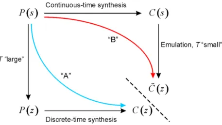
As you learned in class, there are two ways to discretize systems: see Figure 1.
Last week we learned how to emulate a system: this week we learn the discrete time controller synthesis (direct synthesis).
Figure 1: Emulation and Discrete time controller synthesis.
Figure 2: Discrete-time control loop.
The general situation is the following: a control loop is given as in Figure 2.
The continuous time transfer function G(s) is given.
We want to compute the equivalent discrete-time transfer functionH(z). The loop is composed from a Digital-to-Analog Converter (DAC), the continuous-time transfer functionG(s) and an Analog to Digital Converter (ADC).
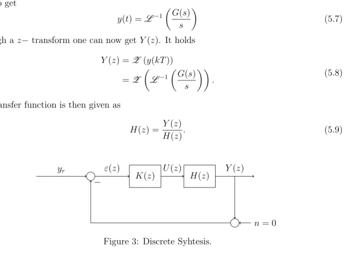
We want to reach a structure that looks like Figure 3.
The first thing to do, is to consider an input to analyze. What is usually chosen, is aunit-step u(kT) ={. . . ,0,1,1, . . .} (5.1) Since the z−Transform is defined as
X(z) =
∞
X
n=0
x(n)·z−n (5.2)
we get for u
U(z) = 1 +z−1+z−2+z−3+. . .+z−n (5.3) This sum can be written as (Analysis I/II)
U(z) = 1
1−z−1 (5.4)
H(z) contains the converters: at first, we have the digital -to-analog converter. The Laplace- Transform of the unit-step reads generally
1
s. (5.5)
Hence, the transfer function before the analog-to-digital converter reads G(s)
s (5.6)
In order to consider theanalog-to-digital converter, we have to apply the inverse Laplace trans- from to get
y(t) =L−1
G(s) s
(5.7) Through a z− transform one can now getY(z). It holds
Y(z) =Z (y(kT))
=Z
L−1
G(s) s
. (5.8)
The transfer function is then given as
H(z) = Y(z)
H(z). (5.9)
K(z) H(z)
yr ε(z) U(z) Y(z)
n= 0
−
Figure 3: Discrete Syhtesis.
6 MIMO Systems
MIMO systems are systems with multiple inputs and multiple outputs. In this chapter we will introduce some analytical tools to deal with those systems.
6.1 System Description
6.1.1 State Space Descriprion
The state-space description of a MIMO system is very similar to the one of a SISO system.
For a linear, time invariant MIMO system with m input signals and poutput signals, it holds d
dtx(t) = A·x(t) +B·u(t), x(t)∈Rn, u(t)∈Rm y(t) = C·x(t) +D·u(t), y(t)∈Rp
(6.1) where
x(t)∈Rn×1, u(t)∈Rm×1, y(t)∈Rp×1, A∈Rn×n, B ∈Rn×m, C ∈Rp×n, D∈Rp×m (6.2) Remark. The dimensions of the matrices A, B, C, D are very important and they are a key concept to understand problems.
The big difference from SISO systems is that u(t) and y(t) are here vectors and no more just numbers. For this reason B, C, D are now matrices.
6.1.2 Transfer Function
One can compute the transfer function of a MIMO system with the well known formula P(s) =C·(s·1−A)−1·B+D (6.3) This is no more a scalar, but ap×n-matrix. The elements of that matrix are rational functions.
Mathematically:
P(s) =
P11(s) · · · P1m(s) ... . .. ... Pp1(s) · · · Ppm(s)
, Pij(s) = bij(s)
aij(s). (6.4)
HerePij(s) is the transfer function from the j-th input to the i-th output.
Remark. In the SISO case, the only matrix we had to care about was A. Since now B,C are matrices, one has to pay attention to some mathematical properties: the matrix multiplication is not commutative(A·B 6=B ·A). Since now P(s) and C(s) are matrices, it holds
L(s) = P(s)·C(s)6=C(s)·P(s). (6.5) Moreover, one can no more define the complementary sensitivity and the sensitivity as
T(s) = L(s)
1 +L(s), S(s) = 1
1 +L(s) (6.6)
because no matrix division is defined. There are however similar expressions to describe those transfer functions: let’s try to derive them.
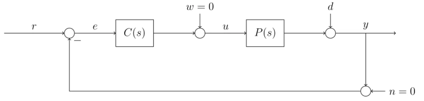
We start from the standard control system’s structure (see Figure 4).
To keep things general, let’s say the plant P(s) ∈Cp×m and the controller C(s)∈ Cm×p. The referencer ∈Rp, the inputu∈Rm and the disturbanced∈Rp. The output Y(s) can as always be written as
Y(s) =T(s)·R(s) +S(s)·D(s) (6.7) where T(s) is the transfer function of the complementary sensitivity and S(s) is the transfer function of the sensitivity.
C(s)
w= 0
P(s)
d
r e u y
n= 0
−
Figure 4: Standard feedback control system structure.
Starting from the error E(s)
If one wants to determine the matrices of those transfer functions, one can start writing (by paying attention to the direction of multiplications) with respect to E(s)
E(s) =R(s)−P(s)·C(s)·E(s)−D(s)
Y(s) =P(s)·C(s)·E(s) +D(s) (6.8)
This gives in the first place
E(s) = (1+P(s)·C(s))−1·(R(s)−D(s)) (6.9) Inserting and writing the functions as F(s) =F for simplicity, one gets
Y =P ·C·E+D
=P ·C·(1+P ·C)−1·(R−D) +D
=P ·C·(1+P ·C)−1·R−P ·C(1+P ·C)−1·D+ (1+P ·C) (1+P ·C)−1
| {z }
1
·D
=P ·C·(1+P ·C)−1·R+ (1+P ·C−P ·C)·(1+P ·C)−1·D
=P ·C·(1+P ·C)−1·R+ (1+P ·C)−1·D.
(6.10)
Recalling the general equation (6.7) one gets the two transfer functions:
T1(s) =P(s)·C(s)·(1+P(s)·C(s))−1
S1(s) = (1+P(s)·C(s))−1 (6.11)
Starting from the input U(s)
If one starts with respect to U(s), one gets
U(s) =C(s)·(R(s)−D(s))−C(s)·P(s)·U(s)
Y(s) =P(s)·U(s) +D(s) (6.12)
This gives in the first place
U(s) = (1+C(s)·P(s))−1·C(s)·(R(s)−D(s)) (6.13) Inserting and writing the functions as F(s) =F for simplicity, one gets
Y =P ·U +D
=P ·(1+C·P)−1·C·(R−D) +D
=P ·(1+C·P)−1·C·R+ 1−P ·(1+C·P)−1·C
·D.
(6.14)
Recalling the general equation (6.7) one gets the two transfer functions:
T2(s) =P(s)·(1+C(s)·P(s))−1·C(s)
S2(s) =1−P(s)·(1+C(s)·P(s))−1·C(s) (6.15) It can be shown that this two different results actually are the equivalent. It holds
S1 =S2
(1+P ·C)−1 =1−P ·(1+C·P)−1·C
1=1+P ·C−P ·(1+C·P)−1·C·(1+P ·C) 1=1+P ·C−P ·(1+C·P)−1·(C+C·P ·C) 1=1+P ·C−P ·(1+C·P)−1·(1+C·P)·C 1=1+P ·C−P ·C
1=1 T1 =T2
P ·C·(1+P ·C)−1 =P ·(1+C·P)−1·C
P ·C=P ·(1+C·P)−1·C·(1+P ·C) P ·C=P ·(1+C·P)−1·(C+C·P ·C) P ·C=P ·(1+C·P)−1·(1+P ·C)·C P ·C=C·P
1=1
(6.16)
Finally, one can show that
S(s) +T(s) = (1+P ·C)−1+P ·C·(1+P ·C)−1
= (1+P ·C)·(1+P ·C)−1
=1
(6.17)
6.2 System Analysis
6.2.1 Lyapunov Stability
The Lyapunov stability theorem analyses the behaviour of a system near to its equilibrium points whenu(t) = 0. Because of this, we don’t care if the system is MIMO or SISO. The three cases read
• Asymptotically stable: limt→∞||x(t)||= 0;
• Stable: ||x(t)||<∞ ∀t≥0;
• Unstable: limt→∞||x(t)||=∞.
As it was done for the SISO case, one can show by using x(t) =eA·t·x0 that the stability can be related to the eigenvalues of A through:
• Asymptotcally stable: Re(λi)<0∀i;
• Stable: Re(λi)≤0∀i;
• Unstable: Re(λi)>0 for at least one i.
6.2.2 Controllability
Controllable: is it possible to control all the states of a system with an input u(t)?
A system is said to be completely controllable, if the Controllability Matrix R = B A·B A2·B . . . An−1·B
∈Rn×(n·m) (6.18)
has full rank n.
6.2.3 Observability
Observable: is it possible to reconstruct the initial conditions of all the states of a system from the output y(t)?
A system is said to be completely observable, if the Observability Matrix
O =
C C·A C·A2
... C·An−1
∈R(n·p)×n (6.19)
has full rank n.
6.3 Poles and Zeros
Since we have to deals with matrices, one has to use the theory ofminors (see Lineare Algebra I/II) in order to compute the zeros and the poles of a transfer function.
The first step of this computation is to calculate all the minors of the transfer function P(s).
The minors of a matrixF ∈Rn×mare the determinants of all square submatrices. By maximal minor it is meant the minor with the biggest dimension. From the minors one can calculate the poles and the zeros as follows:
6.3.1 Zeros
The zeros are the zeros of the numerator’s greatest common divisor of the maximal minors, after their normalization with respect to the same denominator (polepolynom).
6.3.2 Poles
The poles are the zeros of the least common denominator of all the minors of P(s).
6.3.3 Directions
In MIMO systems, the poles and the zeros are related to a direction. Moreover, a zero-pole cancellation occurs only if zero and pole have the same magnitude and input-output direction.
The directions δπ,iin,out associated with a pole πi are defined by P(s)
s=πi ·δπ,iin =∞ ·δπ,iout. (6.20) The directions δξ,iin,out associated with a zero ξi are defined by
P(s)
s=ξi·δξ,iin = 0·δoutξ,i. (6.21) The directions can be computed with thesingular value decomposition (see next week) of the matrix P(S).
6.4 Nyquist Theorem for MIMO Systems
The Nyquist theorem can also be written for MIMO systems. The closed-loop T(s) is asymp- titotically stable if
nc=n++1
2 ·n0 (6.22)
where
• nc: Encirclements about the origin of
N(i·ω) =det(1+P(i·ω)·C(i·ω)) (6.23)
• n+: number of unstable poles.
• n0: number of marginal stable poles.
6.5 Examples
Example 1. The minors of a given matrix P(s) =
a b c d e f
are:
First order:
a, b, c, d, e, f Second order:
det a b
d e
, det a c
d f
, det b c
e f
Example 2. One wants to find the poles and the zeros of the given transfer function P(s) =
s+2
s+3 0
0 (s+1)·(s+3) s+2
Solution. First of all, we list all the minors of the transfer function:
Minors:
• First order: s+2s+3, (s+1)·(s+3)
s+2 , 0, 0 ;
• Second order: s+ 1.
Poles:
The least common denominator of all the minors is (s+ 3)·(s+ 2) This means that the poles are
π1 =−2 π2 =−3.
Zeros:
The maximal minor is s + 1 and we have to normalize it with respect to the polepolynom (s+ 3)·(s+ 2). It holds
(s+ 1) ⇒ (s+ 1)·(s+ 2)·(s+ 3) (s+ 2)·(s+ 3) The numerator reads
(s+ 1)·(s+ 2)·(s+ 3) and so the zeros are
ζ1 =−1 ζ2 =−2 ζ3 =−3.
Example 3. One wants to find the poles and the zeros of the given transfer function P(s) =
1 s+1
1 s+2
2·(s+1) (s+2)·(s+3)
0 (s+1)s+32
s+4 s+1
!
Solution. First of all, we list all the minors of the transfer function:
Minors:
• First order: s+11 ,s+21 ,(s+2)·(s+3)2·(s+1) ,0,(s+1)s+32,s+4s+1;
• Second order: (s+1)s+33,(s+1)·(s+2)s+4 − (s+2)·(s+1)2 = s+11 ,−(s+1)s+42
Poles:
The least common denominator of all the minors is
(s+ 1)3·(s+ 2)·(s+ 3).
This means that the poles are
π1 =−1 π2 =−1 π3 =−1 π4 =−2 π5 =−3 Zeros:
The numerators of the maximal minors are (s+ 3), 1 and−(s+ 4). We have to normalize them with respect to the polepolynom (s+ 1)3·(s+ 2)·(s+ 3). It holds
(s+ 3) ⇒ (s+ 3)2·(s+ 2) (s+ 1)3·(s+ 2)·(s+ 3), 1 ⇒ (s+ 1)2·(s+ 2)·(s+ 3)
(s+ 1)3·(s+ 2)·(s+ 3),
−(s+ 4) ⇒ −(s+ 4)·(s+ 1)·(s+ 2)·(s+ 3) (s+ 1)3·(s+ 2)·(s+ 3) . The greatest common divisor of these is
(s+ 3)·(s+ 2).
Hence, the zeros are
ζ1 =−2 ζ2 =−3
Example 4. The dynamics of a system are given as
˙ x(t) =
4 1 0
−1 2 0
0 0 2
·x(t) +
1 0 0 0 0 1
·u(t) y(t) =
1 0 0 0 1 1
·x(t).
(6.24)
Moreover the transfer function is given as P(s) =
(s−2) s2−6s+9 0
−1 s2−6s+9
1 s−2
!
(6.25) (a) Is the system Lyapunov stable, asymptotically stable or unstable?
(b) Is the system completely controllable?
(c) Is the system completely observable?
(d) The poles of the system are π1 = 2 and π2,3 = 3. The zero of the system is ζ1 = 2. Are there any zero-pole cancellations?
(e) Write aMatlab code that computes the transfer function basing on A, B, C, D.
Solution.
(a)
First of all, one identifies the matrices as:
˙ x(t) =
4 1 0
−1 2 0
0 0 2
| {z }
A
·x(t) +
1 0 0 0 0 1
| {z }
B
·u(t)
y(t) =
1 0 0 0 1 1
| {z }
C
·x(t) + 0 0
0 0
| {z }
D
·u(t)
(6.26)
We have to compute the eingevalues of A. It holds det(A−λ·1) =|
4−λ 1 0
−1 2−λ 0
0 0 2−λ
|
= (2−λ)· |
4−λ 1
−1 2−λ
|
= (2−λ)·((4−λ)·(2−λ) + 1)
= (2−λ)·(λ2−6λ+ 9)
= (2−λ)·(λ−3)2.
Since all the three eigenvalues are bigger than zero, the system is Lyapunov unstable.
(b)
The controllability matrix can be found with the well-known multiplications:
A·B =
4 1 0
−1 2 0 0 0 2
·
1 0 0 0 0 1
=
4 0
−1 0
0 2
,
A2·B =
4 1 0
−1 2 0 0 0 2
·
4 0
−1 0
0 2
=
15 0
−6 0
0 4
. Hence, the controllability matrix reads
R=
1 0 4 0 15 0
0 0 −1 0 −6 0
0 1 0 2 0 4
This has full rank 3: the system ist completely controllable.
(c)
The observability matrix can be found with the well-known multiplications:
C·A =
1 0 0 0 1 1
·
4 1 0
−1 2 0 0 0 2
=
4 1 0
−1 2 2
,
C·A2 =
4 1 0
−1 2 2
·
4 1 0
−1 2 0
0 0 2
=
15 6 0
−6 3 4
.
Hence, the observability matrix reads
O =
1 0 0
0 1 1
4 1 0
−1 2 2 15 6 0
−6 3 4
This has full rank 3: the system ist completely observable.
(d)
Although ζ1 = 2 and π1 = 2 have the same magnitude, they don’t cancel out. Why? Since the system ist completely controllable and completely observable, we have already the minimal realization of the system. This means that no more cancellation is possible. The reason for that is that the directions of the two don’t coincide. We will learn more about this in the next chapter.
(e)
The code reads P=tf(ss(A,B,C,D));
or alternatively P=tf(’s’);
P=C*inv(s*eye(3)-A)*B+D;