Universität zu Köln
Institut für theoretische Physik
Due to, or in spite of? The effect of constraints on efficiency in quantum
estimation problems
Inaugural-Disseration Erlangung des Doktorgradeszur
der Mathematisch-Naturwissenschaftlichen Fakultät der Universität zu Köln
vorgelegt von
Daniel Süß
aus Dresden Köln, 2018
Berichterstatter (Erstgutachter): Prof. David Gross Berichterstatter (Zweitgutachter): Prof. Johannes Berg
Tag der Disputation: 13. September 2018
Abstract
In this thesis, we study the interplay of constraints and complexity in quantum esti- mation. We investigate three inference problems, where additional structure in the form of constraints is exploited to reduce the sample and/or computational com- plexity. The first example is concerned with uncertainty quantification in quantum state estimation, where thepositive-semidefinite constraint is used to construct more powerful, that is smaller, error regions. However, as we show in this work, doing so in an optimal way constitutes a computationally hard problem, and therefore, is intractable for larger systems. This is in stark contrast to the unconstrained version of the problem under consideration. The second inference problem deals with phase retrieval and its application to characterizing linear optical circuits. The main chal- lenge here is the fact that the measurements are insensitive to complex phases, and hence, reconstruction requires deliberate utilization of interference. We propose a reconstruction algorithm based on ideas fromlow-rank matrix recovery. More specif- ically, we map the problem of reconstruction from phase-insensitive measurements to the problem of recovering a rank-one matrix from linear measurements. For the efficient solution of the latter it is crucial to exploit the rank-one constraint. In this work, we adapt existing work on phase retrieval to the specific application of char- acterizing linear optical devices. Furthermore, we propose a measurement ensemble tailored specifically around the limitations encountered in this application. The main contribution of this work is the proof of efficacy and efficiency of the proposed proto- col. Finally, we investigate low-rank tensor recovery – the problem of reconstructing a low-complexity tensor embedded in an exponentially large space. We derive a sufficient condition for reconstructing low-rank tensors from product measurements, which relates the error of the initialization and concentration properties of the mea- surements. Furthermore, we provide evidence that this condition is satisfied with high probability by Gaussian product tensors with the number of measurements only depending on the target’s intrinsic complexity, and hence, scaling polynomially in the order of tensor. Therefore, the low-rank constraint can be exploited to dramatically reduce the sample complexity of the problem. Additionally, the use of measurement tensors with an efficient representation is necessary for computational efficiency.
Kurzzusammenfassung
In dieser Arbeit untersuchen wir das Zusammenspiel von Zwangsbedingungen und Komplexität in Quantenschätzproblemen. Für diesen Zweck betrachten wir drei Schätzprobleme, deren zusätzliche Struktur in der Form von Zwangsbedingungen ausgenutzt werden kann um die notwendige Zahl der Messungen oder die Berech- nungskomplexität zu verringern. Das erste Beispiel beschäftigt sich mit der Un- sicherheitsabschätzung in Quantenzustandstomographie. In diesem nutzen wir die Zwangsbedingung, dass physikalische gemischte Zustände durch positiv-semidefinite Matrizen beschrieben werden, um kleinere und damit aussagekräftigere Fehlerregio- nen zu konstruieren. Wir zeigen jedoch in dieser Arbeit, dass ein optimales Nutzen der Zwangsbedingungen ein rechnerisch schweres Problem darstellt und damit nicht effizient lösbar ist. Im Vergleich dazu existieren effiziente Algorithmen für die Berech- nung optimaler Fehlerregionen im Falle des Models ohne Zwangsbedingungen. Das zweite Schätzproblem beschäftigt sich mitPhase Retrievalund dessen Anwendung für die Charakterisierung vonlinear-optischen Schaltkreisen. Hier ist die größte Heraus- forderung, dass die Messungen phasenunempfindlich sind und deshalb das gezielte Ausnutzen von Interferenz für die vollständige Rekonstruktion notwendig ist. Für diesen Zweck entwickeln wir einen Algorithmus, der auf Techniken der effizienten Rekonstruktion von Matrizen mit niedrigem Rang basiert. Genauer gesagt bilden wir das Problem der Rekonstruktion aus phasenunempfindlichen Messungen auf das Problem der Rekonstruktion von Matrizen mit Rang 1 aus linearen Messungen ab.
Für dessen effiziente Lösung ist es notwendig die Zwangsbedingung an den Rang auszunutzen. Hierzu adaptieren wir existierende Arbeiten aus dem Bereich des Phase Retrievals für die Anwendung auf die Charakterisierung von linear-optischen Schaltkreisen. Außerdem entwickeln wir ein Ensemble von Messvektoren, das speziell auf diese Anwendung zugeschnitten ist. Zuletzt untersuchen wir die Rekonstruk- tion vonTensoren mit niedrigem Rang, also das Problem einen Tensor mit niedriger Komplexität in einem exponentiell großem Hilbertraum zu rekonstruieren. Wir leiten eine hinreichende Bedingung für die erfolgreiche Rekonstruktion von Tensoren mit niedrigem Range aus Rang 1 Messungen ab, die den erlaubten Fehler der Initial- isierung und Konzentrationseigenschaften der Messungen miteinander in Verbindung setzt. Außerdem zeigen wir numerisch, dass Gauss’sche Produktmessungen diese Eigenschaft mit hoher Wahrscheinlichkeit erfüllen, auch wenn die Zahl der Messun- gen polynomiell in der Ordnung des Zieltensors skaliert. Damit können die Rangbe- dingungen ausgenutzt werden um die Zahl der notwendigen Messungen drastisch zu
Contents
1. Introduction 1
2. Uncertainty quantification for quantum state estimation 5
2.1. Introduction to statistical inference . . . 7
2.1.1. Frequentist statistics . . . 7
2.1.2. Bayesian statistics . . . 11
2.2. Introduction to computational complexity theory . . . 13
2.3. Introduction to QSE . . . 18
2.3.1. Existing work on error regions . . . 19
2.3.2. The QSE statistical model . . . 20
2.4. Hardness results for confidence regions . . . 21
2.4.1. Optimal confidence regions for quantum states . . . 22
2.4.2. Confidence regions from linear inversion . . . 24
2.4.3. Computational intractability of truncated ellipsoids . . . 28
2.4.4. Proof of Theorem 2.14 . . . 29
2.5. Hardness results for credible regions . . . 37
2.5.1. MVCR for Gaussian distributions . . . 38
2.5.2. Bayesian QSE . . . 39
2.5.3. Computational intractability . . . 40
2.5.4. Proof of Theorem 2.21 . . . 42
2.6. Conclusion & outlook . . . 50
3. Characterizing linear-optical networks via PhaseLift 53 3.1. Device characterization . . . 54
3.2. Phase retrieval . . . 56
3.3. Theory . . . 59
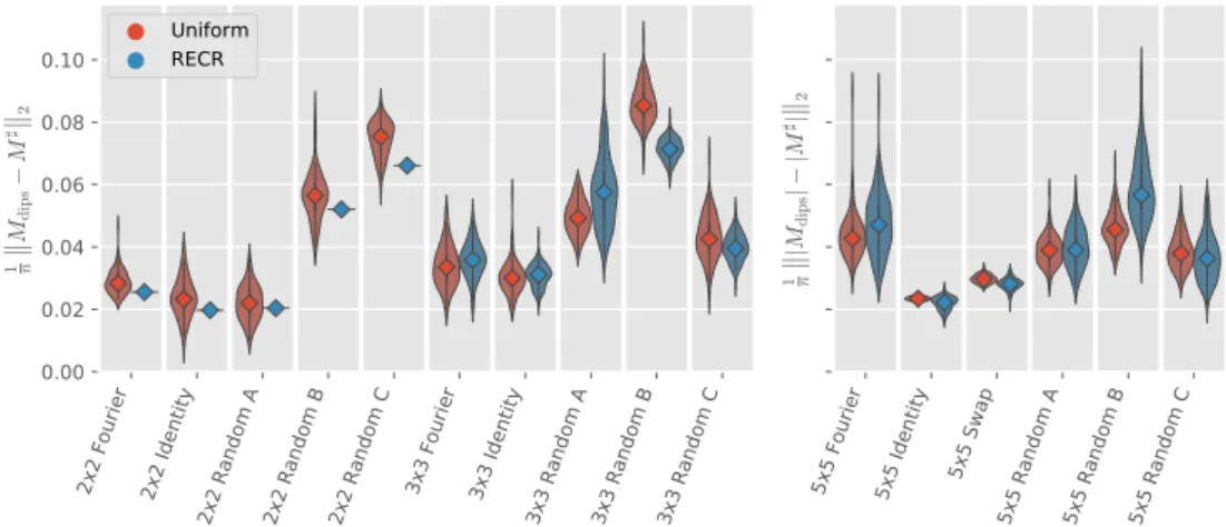
3.3.1. The RECR ensemble . . . 59
3.3.2. Proof of Proposition 3.3 . . . 67
3.3.3. Characterization via PhaseLift . . . 73
3.4. Application . . . 77
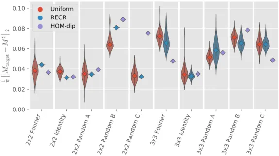
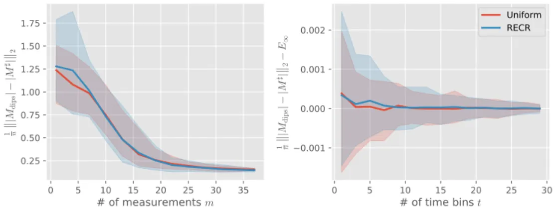
3.4.1. Numerical results . . . 77
3.4.2. Experimental results . . . 80
3.5. Conclusion & outlook . . . 84
4. Low-rank tensor recovery 87
4.1. Matrix Product States . . . 88
4.1.1. Graphical notation . . . 88
4.1.2. MPS tensor representation . . . 89
4.1.3. Applications of the MPS format . . . 94
4.2. The Python Library mpnum . . . 97
4.2.1. The MPArray class . . . 98
4.2.2. Arithmetic Operations . . . 100
4.3. Efficient low-rank tensor reconstruction . . . 103
4.3.1. Existing work . . . 103
4.3.2. The alternating least squares algorithm . . . 107
4.3.3. Analysis of the ALS . . . 109
4.3.4. Gaussian measurements . . . 118
4.3.5. Numerical reconstruction . . . 127
4.4. Conclusion & outlook . . . 131
5. Conclusion 135 A. Appendix 139 A.1. Generalized Bloch representation . . . 139
A.2. Experimental details . . . 139
A.2.1. Reference Reconstructions . . . 139
A.2.2. Data analysis . . . 140
A.3. Meijer G-functions . . . 141
Bibliography 143
1. Introduction
Physics as an inherently empirical science relies on experimental data to single out theories that are compatible with observations. It is therefore a fundamental problem to transform data into answers to questions posed by the physicist. A large fraction of experimental problems can be phrased in terms of parametric estimation: Given a mathematical model that relates the parameters of interest to observable outcomes, estimate the parameters that fit the data “best”. In other words, parameter estima- tion is an inverse problem for a fixed model of the system.
Two crucial aspects of estimation problems in general are constraints and com- plexity. The former refers to the fact that many models are specified in terms of continuous parameters, but not all parameter values correspond to valid models. One typical example for constraints are mathematical facts, e.g. the standard deviationσ of a Gaussian distribution N(µ, σ) should be positive. Others include assumptions on the particular model such as the constraint that a valid density matrix of a quan- tum system is positive semi-definite. Note that not all constraints need to be hard constraints as the examples stated above. Soft constraints can be used to promote desired properties of the estimate or to penalize values due to prior knowledge.
In general, the notion of complexity refers to the amount of resources required to solve inference problems as the size of the underlying models grows. On the one hand, we use “complexity” to refer to the amount of experimental resources required, which is often phrased in terms of sample complexity, i.e. the number of measurements.
Also, other measures such as the time required to perform a given experiment are possible if the necessary information can be quantified. On the other hand, we are interested in the amount of computational resources required to extract the desired information from the available data. Theses are often quantified in terms of runtime of the inference computation. Note that these two notions of complexity can be strongly related: If an experiment – such as the ones performed at the LHC – truly deserves the ubiquitous “Big Data” label, then an enormous amount of computational resources is necessary to perform even simple computations on the whole dataset. Additionally, inference problems can also be intrinsically hard to solve such as inference in general Bayesian networks [Coo90; Rot96].
In this work, we are interested in the interaction of constraints and complexity. The main motivation stems from recent progress in quantum technologies in general and quantum computing in particular: Many established techniques for characterization – i.e. inferring a complete description of a system from experimental data – work well
for small systems with only a few qubits, which were prevalent in the past. However, many of these approaches do not scale to larger systems as they require exponentially large amounts of resources. With the recent announcements of quantum devices with up to 72-qubits [Con18], it becomes clear that new techniques for characterization need to be developed. One way to go forward is to exploit physical constraints or to impose additional assumptions on the model to reduce the amount of resources necessary or to improve estimates. To better understand the interplay of constraints and complexity, we investigate three inference problems with applications to quantum estimation in this work.
In Chapter 2, we examine uncertainty quantification in quantum state estimation – the problem of estimating the density matrix ρ of a quantum system from mea- surements. Since all outcomes of quantum measurements are inherently random, one should not only report the final estimate, but also answer the question whether the result is statistically reliable or simply arose due to chance. For this purpose, we use the notion of “error bars” or “error regions” from statistical inference. To in- vestigate the effects of constraints on the computational complexity of the problem, we consider models that allow for easily computable optimal error regions in the un- constrained case. For those models, we show that taking into account the physical constraints on ρ, i.e. positive semi-definiteness, renders the problem of computing optimal error regions intractable. We also show that there are settings, where ex- actly those physical constraints drastically improve the power of error regions, and therefore, are necessary for optimality. In conclusion, we show that exploiting the physical constraints onρ is essential to obtain optimal error regions, but doing so in an optimal way poses an intractable computational problem in general.
The second main result of this thesis is concerned with characterizing linear optical circuits, which have been proposed as one possible architecture for quantum comput- ing. By measuring the output of such a device for different inputs, the problem is to reconstruct the transfer matrix of the device. Here, the main challenge is that the standard measurement devices in optics – single photon detectors and photo diodes – are insensitive to the phases of the output. Therefore, we need to deliberately use interference between different modes of the device to gain information on the complex phases. This raises the question of how to choose the inputs in an optimal way, in order to reduce the total number of measurements required, and how to reconstruct the transfer matrix in a computationally efficient way. In Chapter 3, we propose a characterization method that is asymptotically optimal w.r.t. the sample complexity, comes with a rigorous proof of convergence, and is robust to noise. The suggested method adapts ideas from low-rank matrix recovery and leverages an exact mathe- matical constraint on the signal to be recovered to derive a reconstruction algorithm that is efficient w.r.t. both sample and computational complexity.
Chapter 4 is dedicated to efficiently reconstructing low-rank tensors from linear measurements. As a natural extension of low-rank matrix recovery, this challeng-
ing problem has received a lot of attention recently. Here, we consider tensors X∈ Rd⊗N
, wheredis the local dimension andN the order of the tensor. Without any additional structure, reconstructingXfrom measurements of the formhA, Xifor measurement tensorsArequires at leastdN such overlaps as each component ofX is independent from the other. Therefore, the sample complexity scales exponentially inN and the problem becomes infeasible already for moderate values ofN. Further- more, any reconstruction algorithm of an arbitrary tensor requires an exponentially long runtime as simply outputting the result takes this amount of time. However, many tensors naturally occurring, e.g. in quantum physics, have additional structure that can be used to render their description and reconstruction efficient. Here, we consider low-MPS rank tensors, which are a generalization of low-rank matrices and constitute a variational class of tenors that have an efficient description in terms of the matrix product state (MPS) representation. More precisely, the number of parameters required to express a tensor of fixed MPS rank in said representation scales linearly inN. The question we are trying to answer is whether such low-MPS rank tensors can be recovered fromm linear measurements such that mscales poly- nomially in the intrinsic complexity, i.e. polynomially in N, instead of depending on the dimension of the embedding space. Additionally, we want the reconstruction algorithm to be efficient. For this purpose, it is necessary to consider measurement tensorsAthat also have an efficient representation, e.g. in the MPS tensor format. In this work, we provide a partial answer to this question We derive a condition on the measurement tensors that is sufficient for recovery via an alternating-minimization algorithm. Numerically, show that random Gaussian product tensors are a viable candidate for measurement tensors fulfilling this condition. The role of the low-MPS rank constraint in this problem is in stark contrast to Chapter 2, where imposing constraints on the parameter to be inferred rendered the problem computationally intractable. Here, the problem of tensor recovery only becomes tractable with the additional low-rank constraint.
2. Uncertainty quantification for quantum state estimation
Due to the intrinsic randomness of quantum mechanics, any information we obtain about a quantum system through measurements is subject to statistical uncertainty.
Consequently, one should not only report the final result of an experiment, but also answer the question whether this result is statistically reliable or simply arose due to chance. This motivated the recent development of techniques for uncertainty quan- tification in quantum state estimation (QSE) [Blu12; Fer14a; Sha+13; FR16; CR12;
AS09; Aud+08]. Despite the large body of work concerned with this problem, none of these constructions are known to be both optimal and computationally feasible.
In this chapter, we investigate the question whether the lack of an efficient algo- rithm for computing optimal error regions in QSE simply is due to a lack of imagi- nation or if there are fundamental restrictions that prevent the existence of such an algorithm. We provide evidence that the latter case is true: Based on the generally accepted conjecture thatP6=NPin computational complexity we show that no such algorithm can exist. More specifically, we show that the computational intractability does not simply arise due to the general difficulties of statistics in high dimensions.
Instead, by considering models which render the unconstrained problem tractable, we show that the computational intractability is caused by the quantum mechanical shape constraints: For%to constitute a valid quantum state, it has to be a Hermitian, positive semi-definite (psd) matrix with unit trace. The Hermiticity and trace con- straints are linear and easily satisfiable by means of a suitable linear parametrization.
In contrast, the psd constraint is non-linear, and hence, more problematic to satisfy.
The motivation for studying uncertainty quantification under quantum constraints is that these constraints can lead to a significant reduction in uncertainty. This is particularly evident if the true state is close to the boundary of state space, e.g. in the case of almost pure states, which are of interest in quantum information processing experiments. In this case, it is plausible that a large fraction of possible estimates that seem compatible with the observations can be discarded, as they lie outside of state space.
Indeed, it is known that taking the quantum constraints into account can result in a dramatic – even unbounded – reduction in uncertainty. Prime examples are results that employ positivity to show that even informationally incomplete measurements can be used to identify a state with arbitrarily small error [Cra+10; Gro+10; Gro11;
Fla+12; NG+13; KKD15]. More precisely, these papers describe ways to rigorously bound the size of a confidence region for the quantum state based only on the ob- served data and on the knowledge that the data comes from measurements on a valid quantum state. While these uncertainty bounds can always be trusted with- out further assumptions, only in very particular situations have they been proven to actually become small. These situations include the cases where the true state is of low rank [Fla+12; NG+13], or admits an economical description as a matrix-product state [Cra+10]. It stands to reason that there are further cases – not yet identified – for which the size of an error region can be substantially reduced simply by taking into account the quantum shape constraints.
Throughout this work, we consider the task of non-adaptive QSE, where a fixed set of measurements specified by the choice of positive operator valued measure (POVM) is performed on independent copies of the system. For a given POVM, the measure- ment outcomes of this setup can be described in terms of a generalized linear model (GLM) with parameter % – the quantum mechanical state or density matrix of the system. The well-established theory of GLMs then provides methods for inferring
% [MN89].
However, what sets the task of QSE apart from inference in GLMs in general are the additional quantum mechanical shape constraints. Nevertheless, there are esti- mators for%that on the one hand always yield a psd density matrix, and on the other hand, are well-understood theoretically with near-optimal performance and scalable to intermediate sized quantum experiments [PR04]. Unfortunately, the same cannot be said for error bars for %.
This chapter is structured as follows: We introduce the necessary concepts from statistical inference and computational complexity in Section 2.1 and 2.2, respectively.
Then, in Section 2.3 we provide more details on QSE and the One of the main results of this work concerning the proof of computational intractability of frequentist confidence region is given in Section 2.4. The Bayesian counterpart for credible regions is the topic of Section 2.5. Finally, we conclude this chapter with remarks on limitations of the hardness results as well as possible future work in Section 2.6.
Relevant publications
• D. Suess, Ł. Rudnicki, T. O. Maciel, D. Gross: Error regions in quantum state tomography: computational complexity caused by geometry of quantum states, New J. Phys. 19 093013 (2017)
2.1. Introduction to statistical inference
2.1. Introduction to statistical inference
The objective of statistical inference is to obtain information about the distribution of a random variableX from observational data. Here, we focus on the special case of inference in parametric models, which can be described as follows [Was13]: A parametric model is a family of distributions {Pθ}θ∈Ω labeled by a finite number of parameters θ, where Ω ⊆Rk is called the state space of the model. For simplicity, we only consider the scalar case k = 1 for now. Then, any function θˆ mapping observations to the spaceRcontaining the parameter space is called apoint estimator for the parameter θ. In general, we do not require θˆto map to the state spaceΩ as this restriction would preclude many relevant estimators such as the linear inversion estimator introduced in Section 2.4.2. However, since we are interested in learning about the distribution of X, not every estimator is equally useful. Indeed, the goal should be to find an estimator, which yields the parameter value that describes the observed data best. What we mean by “best” in this context not only depends on the specific model and what the estimate is supposed to be used for, but also on the fundamental interpretation of probability. Broadly speaking, there are two different interpretations of probability, namely the frequentist (or orthodox) interpretation and the Bayesian interpretation [Háj12], which lead to distinct schools of inference [Kie12;
BC16; Was13]. Although the two approaches yield the same results for very simple models or – under mild regularity assumptions – in the limit of many measurements, they generally differ and in some cases even yield contradictory results [Was13, Sec.
11.9].
So far we have only discussed point estimators, which yield a single value for the parameters. However, even if our model describes the data perfectly for some choice ofθ, we cannot exactly recover this value from a finite amount of data due to statistical fluctuations in general. The concept of error bars, or more specifically error regions, allows for quantifying the uncertainty of a given estimate. In Section 2.1.1, we introduce the basic concepts of frequentist inference and the corresponding notion of confidence regions. Section 2.1.2 is concerned with Bayesian inference and the corresponding notion of error regions, namely credible regions.
2.1.1. Frequentist statistics
In the frequentist framework, the probability of an outcome of a random experiment is defined in terms of its relative frequency of occurrence when the number of repetitions goes to infinity [Key07; Kie12]. More precisely, denote the number of repetitions of an experiment byN and the number of times the event under considerationx occurred by nN. Then, a frequentist interprets the probability P(x) as the statement that
nN
N →P(x) asN → ∞.
For the task of parameter estimation, we assume that the model is well-specified,
i.e. that the observed data are generated from the parametric model with the fixed
“true” parameter θ0 ∈ Ω, which is unknown. From a finite number of observations X1, . . . XN, we must construct an estimate θ(Xˆ ) for θ0. Although there are some intuitive approaches to this problem such as the method of moments [Was13, Sec.
9.2], theprinciple of maximum likelihood is often employed to construct an estimator with good frequentist properties. First, let us introduce thelikelihood functionof the model
L(θ;X) =Pθ(X) =
N
Y
i=1
Pθ(Xi), (2.1)
where we have assumed independence of the samples for the second equality. The maximum likelihood estimator (mle) is then defined by1
θˆMLE(x) = argmaxθ∈ΩL(θ;x). (2.2) The justification for using (2.2) is that under mild conditions on the model, the MLE posses many appealing properties [Was13, Sec. 9.4] such as consistency and efficiency:
Consistency means that the MLE converges to the true value θ0 in probability as N → ∞ and efficiency roughly means that among all well behaved estimators, the MLE has the smallest variance in the large sample limit.
A more flexible approach to the problem of how to single out a “good” estimator is formalized in statistical decision theory [CB02; LC98]. For this purpose, we need to introduce aloss function
L: Ω×R→R,(θ0,θ)ˆ 7→ L(θ0,θ),ˆ (2.3) which measures the discrepancy between the true value θ0 and an estimate θ(Xˆ ).
Keep in mind that since the Xi are random variables, so is θ(Xˆ ) and its loss. In order to asses the estimatorθ, that is the function mapping data to an estimate, weˆ evaluate the average loss orrisk function
R(θ0,θ) =ˆ Eθ0(L(θ0,θ(Xˆ ))) = Z
L(θ0,θ(x))ˆ Pθ0(x) dx. (2.4) Then, the problem of finding a good estimator reduces to the problem of finding an estimator that yields small values for Eq. (2.4). However, note that the risk function (2.4) for a given estimator still depends on the unknown true value. To obtain a single-number summary of the performance of an estimator for all possible values of θ0, there are different strategies such as maximizing or averaging the risk function over all θ0 [Was13, Sec. 12.2]. By minimizing these risks over all possible estimators, we try to determine a single estimator that performs best in the worst case
1Note that we have constrained the values of the MLE to the state spaceΩof the model. Otherwise, the right hand side of Eq. (2.2) might not be well defined.
2.1. Introduction to statistical inference or on average, respectively. However, in the following we introduce a less ambitious notion of optimality, namely admissibility.
Definition 2.1. [Was13, Def. 12.17] A point estimator θˆ is inadmissible if there exists another estimator θˆ0 such that
R(θ0,θˆ0)≤ R(θ0,θ)ˆ for all θ0∈Ω
R(θ0,θˆ0)<R(θ0,θ)ˆ for at least one θ0∈Ω.
Otherwise, we callθˆadmissible.
In words, θˆis admissible if there is no other estimatorθˆ0 that performs at least as good asθˆand strictly better for at least one value of the true valueθ0.
The choice of loss function generally depends on the problem at hand and deter- mines the properties of the corresponding estimator. Some examples for commonly used loss functions include the0/1-loss for discrete parameter models
L(θ0, θ) =
(1 θ0=θ
0 otherwise, (2.5)
and the mean squared error (MSE)
L(θ0, θ) = (θ0−θ)2, (2.6) which is often used for continuous parameter models, e.g. Ω = R. The use of the MSE loss is often motivated by the fact that it gives the same results as the principle of maximum likelihood for many problems. As an example, consider the task of estimating the mean from iid normal random variablesX(k)∼ N(θ0, σ)withσ∈R+
known. In this case, a straightforward estimator forθ0 is theempirical mean X¯ := 1
m
m
X
i=1
X(k), (2.7)
which is admissible with respect to MSE [Was13, Thm. 12.20]. Furthermore, X¯ is also the MLE as a transformation to log-likelihood shows:
argmaxθL(θ;x(1), . . . , x(m)) = argmaxθ
m
X
k=1
logPθ(X(k)=x(k))
= argminθ
m
X
k=1
1 2σ2
x(k)−θ 2
,
(2.8)
where we have used that the X(k) are independent and that the logarithm is mono- tonic increasing. Furthermore, we discarded all contributions independent ofθ is the
second line. Finally, note that the right hand side of the last equation is minimized by the choiceθ= ¯x, which proofs the claim.
Now we consider a multivariate generalization of the above problem, that is the task of estimating θ0 ∈ Rd from a linear Gaussian model X ∼ N(θ0,1) with unit covariance matrix. Suppose we only have a single observation X, i.e. m = 1. Since all the components Xi are independent, one expects that a separate estimation of the components via X¯ =X constitutes a “good estimator”. Indeed, the same com- putation as in Eq. (2.8) shows that the empirical mean is the MLE for this model as well. However, Stein shocked the statistical community when he proved that for d≥3, this estimator is inadmissible [Ste+56]. It can be shown that theJames-Stein estimator
θˆS:= max
0,
1− d−2 kXk2
X (2.9)
has smaller MSE risk than the empirical mean for all values of θ0 [Ste+56; LC98].
It is often referred to as ashrinkage estimator because it shrinks the empirical mean estimate X towards 0. Note however, that the choice of the origin as the fix point of the shrinkage operation is arbitrary – the James-Stein estimator outperforms the empirical mean estimator for any choice of fix point. Interestingly, Eq. (2.9) shows that by taking into account all the componentsXi, we can improve the MSE of the mean-estimator even if theXi are independent. However, this only applies to thesi- multaneousMSE error of all the components ofθ0. The James-Stein estimator (2.9) cannot be used to improve the MSE of a single component. Equation (2.9) can also be generalized to the case of more than one observation, i.e. m > 1. Finally, note that the James-Stein estimator is also not admissible: More elaborate shrinkage es- timators are known to outperform (2.9) w.r.t. the MSE. Even worse, to the best of the author’s knowledge, no admissible construction exists for estimating the mean of ad-variate Gaussian w.r.t. MSE ford≥3.
As already mentioned in the introduction, point estimators cannot convey uncer- tainty in the estimate. For this purpose, we need to introduce a precise notion of
“error bars”, namelyconfidence regions in the framework of frequentist statistics.
Definition 2.2. Consider a statistical model with k parameters, that is Ω⊆Rk. A confidence region C with coverageα∈[0,1]is a region estimator – that is a function that maps observed data x to a subset C(x) ⊆ Rk of the space containing the state space – such that the true parameter is contained in C with probability greater than α:
∀θ0∈Ω :Pθ0(C(X)3θ0)≥1−α. (2.10) Note that the coverage condition (2.10) is not a probabilistic statement about the true parameter θ0 for fixed observed data x. Instead, Definition 2.2 should
2.1. Introduction to statistical inference be interpreted as a statistical guarantee for the region estimator C: Say we repeat an experiment m times and obtain data x(1), …x(M) from a distribution with true parameter θ0. Then, in the limit m→ ∞ at least a fraction of 1−α of the regions C(x(1)), …, C(x(m)) contain the true parameterθ0. In other words, the probabilistic statement in (2.10) refers to the random variableC(X) for fixedθ0.
Similarly to point estimators, Eq. (2.10) does not uniquely determine a confidence region construction. Additional constraints are necessary to exclude trivial construc- tions such as the following: Take the region estimator that is always equal to the full parameter space independent of the data C(X) = Ω, then
Pθ(C(X)3θ0) = 1≥1−α (2.11) for all confidence levels α. Although, this construction trivially fulfils the coverage condition (2.10), it does not provide useful information on the uncertainty as it does not restrict the parameter space at all. Therefore, we have to impose a notion of what constitutes a good confidence region by introducing a loss function. Clearly, if we have two confidence regionsC1 andC2with the same confidence level andC1 ⊂ C2, then C1 is more informative. More generally, smaller regions should be preferred since they convey more confidence in the estimate and exclude more alternatives.
Therefore, measures of size such as (expected) volume or diameter are commonly used as loss functions for region estimators. We now introduce a notion of optimality similar to Definition 2.1.
Definition 2.3. [Jos69, Def. 2.2] A confidence regionCfor the parameter estimation of θ0 ∈Ω is called (weakly) admissible if there is no other confidence region C0 that fulfils
1. (equal or smaller volume) V(C0(x))≤ V(C(x))for almost all observations x.
2. (same or better coverage) Pθ0(C0 3θ0)≥Pθ0(C 3θ0) for all θ0 ∈Ω.
3. (strictly better) strict inequality holds for one θ0 ∈ Ω in (ii) or on a set of positive measure in (i).
This notion of optimality uses “pointwise” volume as a risk function instead of the average volume. The conditions in Definition 2.3 are stated only for “almost all” x since one can always modify the region estimators on sets of measure zero without changing their statistical performance. In Section 2.4.1 we show that this notion of admissibility is especially suitable for studying constrained inference problems.
2.1.2. Bayesian statistics
Let us now introduce the Bayesian point of view on statistical inference: In the Bayesian interpretation, probabilities do not describe frequencies in the limit of in- finitely many repetitions, but they reflect subjective degrees of belief. Put differently,
in the Bayesian framework randomness reflects one’s ignorance or lack of knowledge of the value of a parameter. In contrast to frequentist inference, this enables us to make probabilistic statements about the values of parameters even for a single fixed set of observations. Generally, Bayesian inference for a parametric model is carried out in the following way: First, we choose aprior distribution P(θ), which expresses our belief about the parameterθ before taking any data into account. Given an ob- servationX, the distribution ofθis updated according to Bayes’ rule [BC16; Gel+95]
P(θ|X) = P(X|θ)P(θ)
P(X) . (2.12)
Here, P(X|θ) is the likelihood function of the model analogous to (2.1) and P(θ|X) is the posterior distribution – or short posterior – of θ. Of course, the update in Eq. (2.12) is not limited to a single observation and can be iterated for independent data.
Computing the Bayesian update (2.12) analytically is possible only in a few rare cases: If for a given likelihood function, the prior and the posterior are in the same family of distributions, the prior is called aconjugate priorfor the likelihood function.
For example, consider a Gaussian random variableX∼ N(θ, τ2)with known variance τ2. If we assume a Gaussian prior θ∼ N(µ, σ2), we have [Gel+95, Eq. (2.10)]
θ|X=x∼ N(µ0, σ02) (2.13)
with
µ0 =
µ σ2 +τx2
1 σ2 +τ12
, and σ0 = 1
σ2 + 1 τ2
−1 2
. (2.14)
In other words, an update of a Gaussian prior with a Gaussian likelihood function yields a Gaussian posterior distribution. Although there are other well-known conju- gate priors with explicit formulas for the parameter update, in practice the Bayesian update (2.12) can only be approximated numerically. Commonly used methods in- clude sampling techniques such as Markov Chain Monte Carlo and Sequential Monte Carlo [Gel+95] as well as variational Bayes [FR12].
Note that the posterior distribution encodes all the information on θwe have. To summarize important features of the posterior, we introduce point and region esti- mators similar to the frequentist case: One commonly used estimator is the Bayesian mean estimator (BME) given by
θˆBME(X) = Z
θP(θ|X) dθ. (2.15)
A justification for the BME is that it minimizes (under normal circumstances [LC98;
BGW05]) the expected risk E
R(θ,θ(X))ˆ
, provided the corresponding loss func- tionL is aBregman divergence. Note that the expectation is taken overθ w.r.t. the
2.2. Introduction to computational complexity theory posterior with observation X. Another example of a point estimator is the maxi- mum a posteriori (MAP) estimator. As the name suggests, the MAP estimator is obtained by maximizing the posterior (2.12). Since this does not require the expen- sive computation of the denominator in Eq. (2.12) and – at least local – minima of the posterior can be found efficiently via gradient descent, the MAP estimator is often used for high dimensional problems in machine learning [Mur12] that otherwise would be intractable.
Let us now introduce the appropriate concept of error regions in the Bayesian framework.
Definition 2.4. Acredible region2Cwith credibility1−αis a subset of the parameter space Ωcontaining at least mass 1−α of the posterior
P(θ∈ C|X1, . . . , XN)≥1−α. (2.16) Notice the different notion of randomness compared to Eq. (2.10): Confidence regions are random variables due to their dependence on the data and Eq. (2.10) de- mands that the true value is contained in the confidence region with high probability.
Here, “probability” refers to (possibly hypothetical) repetitions of the experiment – no statement can be made for a single run of an experiment with given outcomes. In contrast, the definition of credible regions (2.16) only refers to probability w.r.t. the posterior, and therefore, is well defined even for a single run of the experiment.
In order to single out “good” credible regions, we need to introduce a notion of op- timality. As argued in Section 2.1.1, smaller error regions are generally more informa- tive. Therefore, good credible regions are minimal-volume credible regions (MVCRs) or credible regions with the smallest diameter. Although in the following we deal with MVCRs w.r.t. a geometric notion of volume, some authors have proposed to measure the volume of a region by its prior probability [EGS06; Sha+13]. In case the posterior has probability density Π w.r.t. the volume measure under consideration, the MVCR is given by highest posterior sets [Fer14a]
C={θ∈Ω : Π(θ)≥λ}. (2.17)
The constantλis determined by the saturation of the credibility level condition (2.16).
2.2. Introduction to computational complexity theory
The objective of computational complexity theory is to classify computational prob- lems according to their inherent difficulty. Broadly speaking, we quantify the diffi- culty by the runtime needed to solve the problem. Other resources, which one may
2We use the same letter for confidence and credible regions when the meaning is clear from the context.
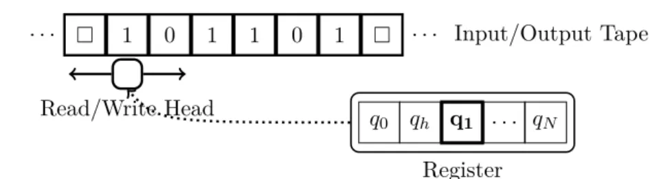
. . . 1 0 1 1 0 1 . . . Input/Output Tape
q0 qh q1 . . . qN Register Read/Write Head
Figure 2.1.: Illustration of a Turing machine with alphabetΓ ={0,1,}and register Q={q0, qh, q1, . . . , qN}.
want to consider, are the amount of memory or communication between parties re- quired.
At a first glance, an answer to the question whether a given problem can be solved efficiently might depend on what we consider as a “computer”: Clearly, a modern high-performance cluster can solve problems in seconds, which would take a human equipped with pen and paper more than a lifetime to finish. Maybe surprisingly, it turns out that a single, simple mathematical model – theTuring machine– describes the capabilities and restrictions of almost all physical implementations of computation well enough for the purpose of complexity theory. The only conceivable exception so far are quantum computers that exploit quantum mechanical phenomena. Although so far no unconditional proof of an advantage of quantum computers exists, there is overwhelming evidence that they are able to solve problems efficiently for which there is no efficient classical algorithm. Note that quantum computers only provide efficient algorithms for problems that are considered hard classically. The class of uncomputable functions is the same for classical and quantum computers [AB09].
This section introduces the main concepts needed for the hardness results of Sec- tion 2.4 and 2.5. Especially the definition ofNP-hard computational problems and polynomial-time reductions is crucial for the rest of this chapter. For a more thorough treatment, we refer the reader to [AB09; GJ79].
A Turing machine (TM) can be thought of as a simplified and idealized mathemat- ical model of an electronic computer. It is defined by a tuple(Γ, Q, δ)and figuratively speaking consists of the following parts as shown in Fig. 2.1:
• An infinite tape, that is a bi-directional line of cells that can take the values from a finite setΓ called the alphabet. Γ must contain a designated symbol called “blank”.
• A register that can take on values from a finite set of statesQ. Qmust contain the initial stateq0 and the halting state qh.
2.2. Introduction to computational complexity theory
• A transition function
δ:Q×Γ→Q×Γ× {L, S, R}, (2.18) which describes the “programming” of the TM.
The operation of a TM can be summarized as follows. Initially, the reading head of the tape is over a certain cell and the register is in the initial stateq0. Furthermore, we assume that only a finite number of tape cells have a value different from – these are referred to as the input. For one step of the computation, denote by γ∈Γ the value of tape cell under the reading head and by q ∈Qthe current value of the register. The action of the TM is determined by the transition function
(q0, γ0, h) =δ(q, γ). (2.19) as follows: The register is set to valueq0, the tape head overwrites the cell with symbol γ0, and it moves depending on the value of h: If h=Lorh=R, it moves one cell to the left or right, respectively and ifh=S it stays in the current position. This cycle repeats until the register takes on the halting state qh. If the TM halts, the state of the tape with leading and trailing blanks removed is taken as its output. Note that the definition of a TM given above is one of many; others may include additional scratch tapes or have tapes that only extend to infinity only in one direction [AB09].
However, they are all equivalent, i.e. the architecture given above can simulate all the other architectures with a small overhead and vice versa. Furthermore, we can assume Γ = {0,1,}, that is, we use a binary encoding for all non-blank values of the alphabet.
We now formalize the notion of runtime of a TM and the complexity of a given problem. Denote by
{0,1}∗ = [
n∈N
{0,1}n (2.20)
the set of all finite bit strings.
Definition 2.5. [AB09, Def. 1.3] Let f:{0,1}∗ → {0,1}∗ and T:N→ N be some functions. Furthermore, let M be a Turing machine. We say M computes f in T(n)-time if for every input x ∈ {0,1}∗, whenever M is initialized with input x, it halts with f(x) written on its output tape in at most T(|x|) steps. Here, |x| denotes the length ofx.
In words, Definition 2.5 gives a formal notion of the runtime of a TM for computing a function f in terms of the number of elemental steps required. But as stated in the introduction, we are more interested in the intrinsic complexity of computing the function f instead of a specific implementation. For this purpose, we introduce complexity classes, which are sets of functions that can be computed within given
resource bounds. The most important examples of complexity classes pertain to boolean functions f:{0,1}∗ → {0,1}, which correspond to decision problems. The corresponding set of “truthy” inputs L={x in{0,1}∗:f(x) = 1} is referred to as a language.
Definition 2.6. Let T: N→ N be some function. We say that a language L is in DTIME(T(n))if and only if there is a TMM that computes f in time c×T(n) for some constant c >0. The complexity class P is then defined by
P= [
λ≥1
DTIME(nλ). (2.21) In words,Pis the set of all languages that can be decided by a TM in a number of steps that scales polynomially in the input size. The problems inPare considered to be efficiently solvable. Therefore, in order to show that some problem is “easy”, we just have to provide a TM, or put differently an algorithm, that decides the problem in polynomial time. On the other hand, showing that no polynomial-time algorithm exists for a given problem shows that it is computationally hard. However, proving the nonexistence of efficient algorithms for many natural computational problems has turned out to be a tremendous challenge – notwithstanding deep results for computa- tional models strictly less powerful than the TM model [AB09, Part Two]. Hence, we are going to follow a less ambitious, but very fruitful strategy: Instead of proving that a given problem is infeasible to solve efficiently, we are comparing its computational complexity to other problems that are conjectured to be computationally infeasible.
If we can show that the problem under consideration is at least as hard as many other problems, which could not be solved efficiently by a myriad of computer scientists in the last decades, then we have strong evidence to believe it is intrinsically hard. This idea is formalized in the definition of polynomial-time reductions.
Definition 2.7. Def. 2.2 from [AB09] A language L ⊆ {0,1}∗ is polynomial- time (Karp) reducible to a Language L0 ⊆ {0,1}∗ denoted by L ≤p L0, if there is a polynomial-time computable functionf:{0,1}∗→ {0,1}∗ such that for allx∈ {0,1}∗ we have x∈L ⇐⇒ f(x)∈L0.
Less formally speaking, if we have L ≤p L0 then L0 is at least as hard to decide asL. Indeed, by using the reduction f, we can turn any TM decidingL0 into a TM deciding L with at most polynomial runtime overhead. Particularly, if additionally L0 ∈P then so is L. Conversely, if no efficient algorithm for L exists and L ≤p L0, then there cannot be an efficient algorithm L0. The latter observation is the basis of the strategy mentioned above: We show that a given problem is computationally hard by establishing that is at least as hard as a large class of other problems, which have withstood numerous attempts at solving them efficiently so far. For this purpose we introduce the complexity classNP.
2.2. Introduction to computational complexity theory Definition 2.8. A language L⊆ {0,1}∗ is in NPif there exists a polynomial-time computable function M such that for every x∈ {0,1}∗
x∈L ⇐⇒ ∃u∈ {0,1}p(|x|)s.t. M(x, u) = 1. (2.22) The function M is called the verifier and for x ∈ L, the bitstring u is called a certificate for x.
Clearly, P ⊆ NP with p(|x|) = 0. On the other hand, the question whether NP⊆P, and hence, P =NP is one of the major unsolved problems in math and science [Coo06; Aar; GJ79]. One argument against this hypothesis goes as follows:
Whereas the problems in P are considered to be easily solvable, the problems in NP are at least easily checkable given the certificate. In other words the question whetherP=NPboils down to the question whether finding the solution to a prob- lem is harder than verifying whether a given solution is correct. However, these philosophical considerations are not the main reason for the importance of Defini- tion 2.8 from a computer scientific point of view. The main justification of the class NPis twofold: On the one hand, there are a myriad of problems known to be inNP and many of them have resisted all efforts of finding a polynomial-time algorithm.
On the other hand, there is a tremendous number of problems known to be at least as hard as any problem inNP[GJ79] – these are referred to as NP-hard problems:
Definition 2.9. We say that a language L is NP-hard if for every L0 ∈ NP we have L0 ≤p L. We say that a language L is NP-complete if L ∈ NP and L is NP-complete.
Clearly, for anyNP-hard problemL,L≤pL0 implies thatL0 is NP-hard as well, and hence, any problem in NP is polynomial-time reducible to L0. Therefore, an efficient algorithm for L0 would provide an efficient algorithm for a large number of other problems, which are widely considered difficult and which have been con- founding experts for years. This fact is taken as very strong evidence thatL0 cannot be solved efficiently. As an example of an NP-complete problem, we consider the number partition problem.
Problem 2.10. Given a vectora∈Nd, decide whether there exists a vector ψ with
∀k ψk∈ {−1,1} and a·ψ= 0. (2.23) In case there is such a vectorψ one says that the instancea allows for a partition because the sum of components ofa labeled byψi = 1is equal to the sum of compo- nentsailabeled byψi=−1. For a proof ofNP-hardness of Problem 2.10, see [GJ79].
The question remains what the notion ofNP-hardness means in practice. Due to its strict definition in terms of worst-case runtime needed for any instance, Defini- tion 2.8 leaves open many possibilities for the existence of “good-enough” solutions.
First, approximative or probabilistic algorithms often suffice for all practical pur- poses and are not bounded byNP-hardness results [GJ79; AB09]. A prime example is the number partition problem 2.10: It is often considered the “easiest hard prob- lem” because although it isNP-hard, highly efficient approximative algorithms for it exist [Kel+03]. Furthermore, considering only the worst-case behavior is often too pessimistic in practice. A more appropriate classification of the difficulty of “typical”
instances is given in terms ofaverage case complexity [AB09].
2.3. Introduction to QSE
The goal of state estimation is to provide a complete description of an experimen- tal preparation procedure from experimental feasible measurements. In the case of QSE, this complete description is given in terms of the density matrix % of the system [PR04]. Another common procedure performed in quantum experiments is quantum process estimation, where the goal is to recover aquantum channel [NC10].
However, the task of process estimation can be mapped to QSE by way of the Choi- Jamiolkowski isomorphism [NC10; JFH03; Alt+03], and therefore, we are only con- cerned with the problem of QSE in this work.
Since its inception in the fifties [Fan57], QSE has proven to be a crucial experi- mental tool – in particular in quantum information-inspired setups. It has been used to characterize quantum states in a large number of different platforms [OBr+04;
Lun+09; Mol+04; KRB08; Rip+08; Ste+06; Chi+06; Rie+07; Sch+14] and even been scaled to systems with dimension on the order of 100 [Häf+05]. However, as the Hilbert space dimensions of quantum systems implemented in the lab grow, it is unclear whether this approach to “quantum characterization” will continue to make sense.
Acquiring and post-processing the data necessary for fully-fledged QSE is already prohibitively costly for intermediated sized quantum experiments. As an extreme ex- ample, the eight qubit MLE reconstruction with bootstrapped error bars in [Häf+05]
required weeks of computation in 2005 (private communication, see [Gro+10]). Some sol This problem can be partially mitigated by means of more efficient algorihtms [SGS12;
Qi+13; Hou+16; SZN17] or approaches exploiting structural assumptions to improve the sampling and computational complexity of state estimation [Cra+10; Gro+10;
Fla+12; Sch+15; Bau+13b; Bau+13a].
There is also the question what use is a giant density matrix with millions of entries to an experimentalist? In many cases, the full quantum state contains more infor- mation than necessary. For example, consider the case when a single number such
2.3. Introduction to QSE as the fidelity of the state in the lab w.r.t. some target state is sufficient whether the experiment works “sufficiently well” or not. For this purpose, a variety of theoreti- cal tools for quantum hypothesis testing,certification, and scalarquantum parameter estimation [OW15; Aud+08; GT09; FL11; Sch+15; Li+16] have been developed in the past years that avoid the costly step of full QSE.
However, there remain use cases that necessitate fully-fledged QSE. We see a partic- ularly important role in the emergent field ofquantum technologies: Any technology requires means of certifying that components function as intended and, should they fail to do so, identify the way in which they deviate from the specification. As an example, consider the implementation of a quantum gate that is designed to act as a component of a universal quantum computing setup. One could use a certifica- tion procedure – direct fidelity estimation, say – to verify that the implementation is sufficiently close to the theoretical target that it meets the stringent demands of the quantum error correction threshold. If it does, the need for QSE has been averted.
However, should it fail this test, the certification methods give no indicationin which way it deviated from the intended behavior. They yield no actionable information that could be used to adjust the preparation procedure. The pertinent question
“what went wrong” cannot be cast as a hypothesis test. Thus, while many estima- tion and certification schemes can – and should – be formulated without resorting to full state estimation, the above example shows that QSE remains an important primitive.
2.3.1. Existing work on error regions
In practice (e.g. [Häf+05]), uncertainty quantification for tomography experiments is usually based on general-purpose resampling techniques such as “bootstrapping” [ET94].
A common procedure is this: For every fixed measurement setting, several repeated experiments are performed. This gives rise to an empirical distribution of outcomes for this particular setting. One then creates a number of simulated data sets by sampling randomly from a multinomial distribution with parameters given by the empirical values. Each simulated data set is mapped to a quantum state using max- imum likelihood estimation. The variation between these reconstructions is then re- ported as the uncertainty region. There is no indication that this procedure grossly misrepresents the actual statistical fluctuations. However, it seems fair to say that its behavior is not well-understood. Indeed, it is simple to come up with pathological cases in which the method would be hopelessly optimistic: E.g. one could estimate the quantum state by performing only one repetition each, but for a large number of randomly chosen settings. The above method would then spuriously find a variance of zero.
On the theoretical side, some techniques to compute rigorously defined error bars
for quantum tomographic experiments have been proposed in recent years. The works of Blume-Kohout [Blu12] as well as Christandl, Renner, and Faist [CR12; FR16]
exhibit methods for constructing confidence regions for QST based on likelihood level sets. While very general, neither paper provides a method that has both a runtime guarantee and also adheres to some notion of non-asymptotic optimality [Kie12; Le 12].Some authors have proposed a “sample-splitting” approach, where the first part of the data is used to construct an estimate of the true state, whereas the second part serves to construct an error region around it [Fla+12] (based on [FL11]), as well as [Car+15b]. These approaches are efficient, but rely on specific measurement ensembles (operator bases with low operator norm), approach optimality only up to poly-logarithmic factors, and – in the case of [Fla+12; FL11] – rely on adaptive measurements.
Regarding Bayesian methods, theKalman filtering techniques of [Aud+08] provide a efficient algorithm for computing credible regions. This is achieved by approximat- ing all Bayesian distributions over density matrices by Gaussians and restricting attention to ellipsoidal credible regions. The authors develop a heuristic method for taking positivity constraints into account – but the degree to which the resulting construction deviates from being optimal remains unknown. A series of recent pa- pers aim to improve this construction by employing the particle filter method for Bayesian estimation and uncertainty quantification [GFF17; Wie+15; Fer14a]. Here, Bayesian distributions are approximated as superpositions of delta distributions and credible regions constructed using Monte Carlo sampling. These methods lead to fast algorithms and are more flexible than Kalman filters with regard to modelling prior distributions that may not be well-approximated by any Gaussian. However, once more, there seems to be no rigorous estimate for how far the estimated credible regions deviate from optimality. Finally, the work in [Sha+13] constructs optimal credible regions w.r.t. a different notion of optimality: Instead of penalizing sets with larger volume, they aim to minimize the prior probability as suggested by [EGS06].
2.3.2. The QSE statistical model
We now introduce the statistical model and the corresponding likelihood function used for the rest of this chapter. The first major assumption is that the system’s state in the lab is sufficiently stable for the duration of the experiment. Therefore, we can assume that all data is generated from a fixed, but unknown state %0 ∈ S, where
S:=
n
%∈Cd×d:%†=%,tr%= 1, %≥0
o (2.24)
denotes the state space of density matrices. Note that this assumption is not neces- sary for QSE in general, see e.g. [GFF17] for Bayesian methods that allow for tracking
2.4. Hardness results for confidence regions time-dependent states.
Since we consider the case of non-adaptive state estimation, the measurements performed are characterized by a fixed POVM {Ek}mk=1 and the probability of the eventk when the system is in the state %0 is given by theBorn rule
pk= trEk%0. (2.25)
However, in reality the quantum expectation values are never observed directly. In- stead, when the experiment is repeated onN independent copies of %0, the observa- tions are counts ni≥0 withP
ini =N following a multinomial distribution Pp(n1, . . . , nm) = N!
n1!· · ·nm!pn11 × · · · ×pnmm. (2.26) In case N is large and all the pi are sufficiently large, the multinomial distribu- tion (2.26) is local asymptotic normal [Sev05]. Therefore, we can approximate Eq. (2.26) by a Gaussian distribution
Pp(y1, . . . , ym)≈Πp,Σ(y1, . . . , ym) (2.27) with yi = nNi and Πp,Σ denoting the probability density of a Gaussian distribution with meanpand covariance matrix Σ = diag(p)−ppT. Hence, under this Gaussian approximation, the relative counts yi are given in terms of a linear Gaussian model with Gaussian likelihood function
L(%;y) =Pp(y) (2.28)
defined in terms of Eq. (2.27) and the probabilitiespk= trEk%. However, if some of thepi are close or equal to zero, which happens for rank deficient%0, local asymtotic normality (LAN) – that is the approximation in Eq. (2.27) – does not hold. In [SB18]
the authors discuss some implications of the lack of LAN in QSE.
2.4. Hardness results for confidence regions
In this section we are going to present the first major result of our work [SRG+17]
concerned with frequentist confidence regions in QSE. Optimal confidence regions for high-dimensional parameter estimation problems in are generally intricate even with- out additional constraints as there are only few elementary settings, where optimal confidence regions are known and easily characterized.
Since the goal of this work is to demonstrate that quantum shape constraints severely complicate even “classically” simple confidence regions, in the further dis- cussion we restrict the discussion to a simplified setting: We focus on confidence ellipsoids for Gaussian distributions, which are one of the few easily characterizable
examples. Furthermore, Gaussian distributions arise in the limit of many measure- ments due to local asymptotic normality. In this section we show that even charac- terizing these highly simplifying ellipsoids with the quantum constraints taken into account constitutes a hard computational problem. This simplification is motivated by the goal to show that the computational intractability exclusively stems from the quantum constraints and that it is not caused by difficulties of high-dimensional statistics in general. Furthermore, any less restrictive formulation encompassing this simplified setting must be at least as hard to solve.
In conclusion, although exploiting the physical constraints may help to reduce the uncertainty tremendously as mentioned in the introduction, doing so in an optimal way is computationally intractable in general. Therefore, our work can be interpreted as a trade-off between computational efficiency and statistical optimality in QSE.
2.4.1. Optimal confidence regions for quantum states
As already indicated in the introduction, additional constraints on the parameter θ0 under consideration can be exploited to possibly improve any confidence region estimator. This is especially clear for notions of optimality with a loss function stated in terms of a volume measureV(·), as we will show in this section. Therefore, assume that θ0 ∈ Ωc, where the constrained parameter space Ωc ⊆ Ω has non-zero measure w.r.t.V. We consider an especially simple procedure to take the constraints into account, namely truncating allθ /∈Ωc from tractable confidence regions for the unconstrained problem.
Although such an ad-hoc approach does not seem to exploit the constraints in an optimal way, it has multiple advantages as we discuss in more detail in Section 2.4.3:
First and foremost, some notions of optimality, e.g. admissibility, are preserved under truncation as shown in Lemma 2.11. In other words, there are notions of optimality such that truncation of an optimal confidence region for the unconstrained problem gives rise to an optimal region for the constrained one. Furthermore, as already men- tioned in the introduction, our goal is to show that the intractability arises purely due taking the constraints imposed by quantum mechanics into account. Therefore, we start from a tractable solution in the unconstrained setting and show that even this simple approach of taking the constraints into account leads to an computationally intractable problem. Finally, the truncation approach simplifies the discussion but as we discuss in Section 2.4.3, our results apply to a much larger class of confidence regions such as likelihood ratio based Gaussian ellipsoids.
We start by showing that the truncation of confidence regions preservers admissi- bility. Notice that Definition 2.3 can be stated for both, the unconstrained estimation problem θ0 ∈ Ω as well as the constrained estimation problem θ0 ∈ Ωc. The ques- tion is: How are admissible confidence regions for the constrained setting related to