Constraints on the tectonic and landscape evolution of the Bhutan Himalaya from thermochronometry
B. A. Adams1, K. V. Hodges1, K. X. Whipple1, T. A. Ehlers2, M. C. van Soest1, and J. Wartho1,3
1School of Earth and Space Exploration, Arizona State University, Tempe, Arizona, USA,2Department of Geosciences, Universität Tübingen, Tubingen, Germany,3GEOMAR Helmholtz Centre for Ocean Research Kiel, Kiel, Germany
Abstract
The observed geomorphology and calculated thermal histories of the Bhutan Himalaya provide an excellent platform to test ideas regarding the influence of tectonics and climate on the evolution of a convergent mountain range. However, little consensus has been reached regarding the late Cenozoic history of the Bhutan Himalaya. Some researchers have argued that observed geologic relationships show slowing deformation rates, such that the range is decaying from a geomorphic perspective, while others see the range as growing and steepening. We suggest that a better understanding is possible through the integrated interpretation of geomorphic and thermochronometric data from the comparison of predictions from models of landscape evolution and thermal-kinematic models of orogenic systems. New thermochronometric data throughout Bhutan are most consistent with a significant decrease in erosion rates, from 2 to 3 km/Ma down to 0.1–0.3 km/Ma, around 6–4 Ma. We interpret this pattern as a decrease in rock uplift rates due to the activation of contractional structures of the Shillong Plateau, an uplifted region approximately 100 km south of Bhutan.However, low-relief,fluvial landscapes throughout the Bhutanese hinterland record a late pulse of surface uplift likely due to a recent increase in rock uplift rates. Constraints from our youngest thermochronometers suggest that this increase in rock uplift and surface uplift occurred within the last 1.75 Ma. These results imply that the dynamics of the Bhutan Himalaya and Shillong Plateau have been linked during the late Cenozoic, with structural elements of both regions active in variable ways and times over that interval.
1. Introduction
The Bhutan Himalaya (Figure 1) is a poorly understood portion of Earth’s largest convergent orogen.
Inconsistent published interpretations of thermochronometric data [Grujic et al., 2006;Long et al., 2012;
McQuarrie et al., 2014;Coutand et al., 2014] and geomorphic observations [Duncan et al., 2003;Baillie and Norbu, 2004; Grujic et al., 2006] frame an interesting conundrum in Bhutan. Is the range decaying as tectonic convergence is accommodated by outboard structures, as some thermochronometry interpretations imply [Clark and Bilham, 2008;Coutand et al., 2014]? Or is Bhutan undergoing a recent period of tectonic rejuvenation and surface uplift as the geomorphology suggests [Duncan et al., 2003;
Baillie and Norbu, 2004]? Or could observed recent surface uplift rather be a landscape response to the development of a rain shadow behind the growing Shillong Plateau [Grujic et al., 2006]?
Currently, three different hypotheses have been proposed for the recent evolution of the Bhutan Himalaya. In thefirst, slowing exhumation rates inferred from thermochronometric data have been interpreted as being caused by reduced fault slip rates within the Bhutan Himalaya as the Shillong Plateau structures to the south became active [Coutand et al., 2014]. For simplicity, we will refer to this asTectonic Decline Hypothesis. A second the,Climate Hypothesis, holds that the same reduction in exhumation rates can be interpreted as a geomorphic response to the formation of a rain shadow north of the Shillong Plateau [Grujic et al., 2006].
Grujic et al. [2006] also posited that several isolated, high-elevation, low-relief landscapes located in the middle latitudes of central and eastern Bhutan could have formed in response to a reduction in erosional efficiency in the rain shadow if rock uplift rates remained constant. Importantly, the Climate Hypothesis holds that western Bhutan lies outside of the rain shadow and should not exhibit the transient landscapes or reduced exhumation rates. Yet another notion, theTectonic Rejuvenation Hypothesis, arose from the sense that the low-relief landscapes were created by changes in fault activity within the Himalaya [Duncan et al., 2003;Baillie and Norbu, 2004] and could have been formed as the result of a recent increase in rock uplift rates.
Unfortunately, it is difficult to simultaneously satisfy thermochronometric constraints on the exhumation history, geomorphic constraints on landscape evolution history, and hydrometeorologic data on rainfall
Tectonics
RESEARCH ARTICLE
10.1002/2015TC003853
Key Points:
•Geomorphic observations show surface uplift has occurred across all of Bhutan
•Bedrock cooling histories show erosion rates slowed across Bhutan circa 6–4 Ma
•Thermochronometry and geomorphology imply surface uplift is driven by tectonics
Supporting Information:
•Readme
•Table S1
•Table S2
•Table S3
•Text S1, Figures S1 and S2, and Tables S1 and S3 captions
Correspondence to:
B. A. Adams,
byron.adams@uni-tuebingen.de
Citation:
Adams, B. A., K. V. Hodges, K. X. Whipple, T. A. Ehlers, M. C. van Soest, and J. Wartho (2015), Constraints on the tectonic and landscape evolution of the Bhutan Himalaya from thermochronometry, Tectonics,34, 1329–1347, doi:10.1002/
2015TC003853.
Received 11 FEB 2015 Accepted 15 MAY 2015
Accepted article online 20 MAY 2015 Published online 30 JUN 2015
©2015. American Geophysical Union.
All Rights Reserved.
and runoff patterns using any single one of the three hypotheses (see Table 1 for summary). Although the Tectonic Decline and Climate hypotheses both provide plausible explanations for at least some of the thermochronometric evidence of a decrease in exhumation rates, there are problems with each. The geomorphology of Bhutan suggests that topographic relief is increasing, which cannot be explained by the Tectonic Decline Hypothesis. In addition, exhumation rates appear to have slowed not only on low- relief surfaces but also in the canyons surrounding them [Coutand et al., 2014], a circumstance that we will show is inconsistent with the Climate Hypothesis. Moreover, the modern rain shadow is only recorded in the foothills of the Bhutan Himalaya; no contrast in rainfall and runoff within the rain shadow is detectable within the interior of Bhutan, where the perched low-relief landscapes are preserved [Baillie and Norbu, 2004], thus weakening the Climate Hypothesis. Finally, no increase in exhumation rate has been observed Figure 1.(a) Digital elevation model of the Bhutan Himalaya. Grey lines mark political boundaries. Fault locations are based on the maps ofLong et al. [2012],Cooper et al. [2012, 2013], andAdams et al. [2013]. JF = Jomolhari fault, STF = South Tibetan fault system, KT = Kakhtang thrust, MCT = Main Central Thrust system, MBT = Main Boundary thrust system, MFT = Main Frontal thrust system, LF = Lhuentse fault, SP = Shillong Plateau. (b) Geomorphic map of the Bhutan Himalaya. Base map is colored according to the ratio of mean elevation to local relief (both calculated with a 5 km diameter window). Thick dashed lines demarcate the boundaries of perched low-relieffluvial landscapes. Blue lines trace the rivers shown in Figure 2, and magenta circles locate significant knickpoints. Thin black lines mark political boundaries.
in the hinterland of Bhutan to lend support to the Tectonic Rejuvenation Hypothesis. In fact, only a decrease in exhumation rates since late Miocene times has been observed in the hinterland [e.g.,Grujic et al., 2006;
Long et al., 2012;McQuarrie et al., 2014;Coutand et al., 2014].
In this paper, we begin with the assumption that a comprehensive model of the late Cenozoic tectonics of Bhutan requires the integration of some aspects of at least two, and perhaps all three, hypotheses. It is not unreasonable to expect that the Tectonic Decline and Climate hypotheses might operate in conjunction as both the dissipation of shortening and uplift rates within the Bhutan Himalaya and the formation of a rain shadow would reasonably result from the formation of the Shillong Plateau. Also, although the present rain shadow is restricted to the foothills, it is plausible that the interior of Bhutan did receive greater rainfall prior to the uplift of the Shillong Plateau. A recent tectonic rejuvenation of the Bhutan Himalaya could plausibly follow an earlier deceleration (Tectonic Decline and Tectonic Rejuvenation hypotheses linked sequentially). Moreover, a tectonic rejuvenation event young enough to be recorded in the transient landscape morphology might not be recorded in the thermal history of surface samples; thermochronometric data from surface samples can only record an acceleration in exhumation rate if the total amount of exhumation since the acceleration exceeds the depth of the closure isotherm at the onset of rapid exhumation.
Fortunately, the results of landscape evolution experiments suggest there is a way to determine which of these hypothetical scenarios most accurately describes the evolution of the Bhutan Himalaya. As we review below, the results of physical [Bonnet and Crave, 2003] and numerical models [Whipple and Tucker, 1999; Whipple, 2001] predict clearly distinguishable end-member erosion histories in response to a decrease in the rock uplift rate (Tectonic Decline Hypothesis), an increase in the rock uplift rate (Tectonic Rejuvenation Hypothesis), a decrease in the precipitation rate (Climate Hypothesis), or a combination of aspects of each. To test the plausibility of these hypotheses, we utilize a multichronometer approach (apatite (U-Th)/He [ApHe], zircon (U-Th)/He [ZrnHe], and muscovite 40Ar/39Ar [MsAr]) and thermal- kinematic modeling to improve the temporal resolution of exhumation histories in Bhutan. We leverage these data with landscape evolution models to help resolve the apparent incompatibility of thermochronometric and geomorphic observations in Bhutan. Ultimately, we show that the integration of thermochronologic and geomorphic studies can be used to achieve a comprehensive understanding of the late Cenozoic evolution of Bhutan in a way that studies of either kind alone cannot.
2. Tectonic and Geomorphic Setting
2.1. Tectonic History of the Eastern Himalaya and Shillong Plateau
While the age of collision between India and Eurasia is still debated [e.g.,Aitchison et al., 2007;Bouilhol et al., 2013,Tripathy-Lang et al., 2013], it is commonly accepted that the major contractional structures south of the Table 1. Proposed Mechanisms for the Recent Tectonic and Landscape Evolution of the Bhutan Himalaya
Hypotheses Description Predictions Sources
Climate Surface uplift caused by reduction in erosional efficiency in the Shillong Plateau rain shadow.
Exhumation rates decreased rapidly in central and eastern Bhutan and then rebounded as knickpoints
migrated headward. No change in the west.
Landscapes upstream of the knickpoint erode slowly and are uplifted.
Baillie and Norbu[2004] and Grujic et al. [2006]
Tectonic Decline Indo-Eurasian convergence on Shillong Plateau structures reduced deformation within the
Himalayan range.
Exhumation and fault slip rates decrease in the Himalayan
range north of active outboard structures.
Grujic et al. [2006] and Coutand et al. [2014]
Tectonic Rejuvenation An increase in tectonic activity led to surface uplift and higher exhumation rates.
Exhumation rates increased as knickpoints migrated headward. Landscapes upstream of the knickpoint
eroded slowly and were uplifted.
Duncan et al. [2003] and Baillie and Norbu[2004]
Hybrid Indo-Eurasian convergence on Shillong Plateau structures reduced rock uplift rates within the Himalayan range. This period was followed by an increase in rock uplift rates and surface uplift.
Exhumation rates decreased in the Himalayan range north of active outboard structures. Landscapes later adjusted to higher rock uplift rates by increasing
erosion rates and undergoing surface uplift.
this study
Himalayan crest have been active since at least the Early Miocene [e.g., Hodges, 2000]. The regional geology of the south flank of the Himalaya can be simplified into three tectonostratigraphic units that increase in metamorphic grade northward and are divided by three south vergent thrust systems (Figure 1a). The Main Frontal thrust system carries essentially unmetamorphosed rocks of the sub-Himalayan foreland in its hanging wall over Gangetic basin units in its footwall.
Moving up section, and northward, are the Main Boundary and Main Central thrust systems.
The Main Boundary thrust hanging wall contains predominantly metasedimentary rocks of the Lesser Himalayan sequence. The metamorphic grade of these rocks increases northward to lower amphibolite facies near the trace of the overlying Main Central thrust sheet. The hanging wall of that structure contains higher-grade (amphibolite to granulite facies) orthogneisses and paragneisses of the Greater Himalayan sequence. Ages of initiation of the Main Central, Main Boundary, and Main Frontal thrust systems are thought to be circa 23, 10, and 5 Ma, respec- tively [e.g.,Hodges, 2000;Long et al., 2012].
South of the eastern Himalaya, a number of structures related to the emergence of the Shillong Plateau add complexity to the regional deformational pattern. A particularly significant deformational feature is the north dipping Dauki thrust system, the trace of which marks the southern margin of the Shillong Plateau (Figure 1) [Biswas and Grasemann, 2005]. The system of faults associated with the Shillong Plateau uplift broadens and extends northeastward from the western edge of the plateau (approximately 90°E) to the Indo-Burman Ranges [Seeber and Armbruster, 1981; Biswas et al., 2007; Clark and Bilham, 2008; Banerjee et al., 2008].
Previous estimates of the timing of uplift of the Shillong Plateau have ranged from circa 8–15 Ma [Biswas et al., 2007;Clark and Bilham, 2008;Avdeev et al., 2011].
Nevertheless, global positioning satellite constraints on the regional modern velocityfields suggest that contractional structures south of the Main Frontal thrust trace may accommodate up to 8 mm/a of continental convergence in the eastern portions of the orogenic system, whereas convergence rates in Bhutan on Himalayan structures are approximately 14–17 mm/a [Vernant et al., 2014]. Contraction rates across the Shillong Plateau estimated on geological timescales using thermochronometric techniques have ranged from 0.65 to 2.3 mm/a since the late Miocene [Biswas et al., 2007;Clark and Bilham, 2008]. The discrepancy between these long-term rates and the modern is suggestive of a recent acceleration of slip rates on the Shillong Plateau structures [Banerjee et al., 2008; Vernant et al., 2014], which may have occurred circa 8–4 Ma [Vernant et al., 2014]. Interestingly,Coutand et al. [2014] utilized bedrock cooling histories in eastern Bhutan to show that overthrusting velocities were nearly halved around 6 Ma, and attributed this slow down to shortening accommodated by the Shillong Plateau (consistent with the Tectonic Decline Hypothesis).
2.2. Transient Landscapes of Bhutan
Digital topographic analysis andfield studies have illuminated low-relief landscapes that are perched above deeply incised canyons and are widespread throughout the middle latitudes of Bhutan [Duncan et al., 2003;
Baillie and Norbu, 2004;Grujic et al., 2006;Adams et al., 2013]. Topographic metrics (hillslope angle, local relief, channel steepness, and mean elevation) analyzed using the methods ofAdams et al. [2013] show that perched, fluvial, low-relief landscapes with similar characteristics and occurring at similar elevations, extend into western Bhutan (Figure 1b). While the low-relief surface in western Bhutan is not asflat or high as the other low-relief surfaces (see Figures 1a and 1b), the river profiles from this region show a dramatic transient form. Longitudinal river channel profiles (Figure 2) clearly reflect these low-relief landscapes upstream of knickpoints across western Bhutan (Figure 2). Downstream of the low-relief Figure 2.River profiles across the Bhutan Himalaya. See Figure 1b
for river traces. Open circles mark the significant slope-break knick- points, which separate regions of high and low channel steepness.
landscapes, mean elevations quickly fall and local relief increases (Figure 1b), indicative of headward propagating slope-break knickpoints (Figure 2) [Baillie and Norbu, 2004;Grujic et al., 2006;Adams et al., 2013].
These knickpoints, which separate terrains with different channel steepness indices (Figure 2), suggest that there has been significant surface uplift between approximately 89°E–91.5°E [e.g.,Whipple and Tucker, 1999;
Kirby and Whipple, 2012].
Grujic et al. [2006] suggested that the transient landscapes and decrease in Late Miocene exhumation rates, as recorded by apatitefission track (ApFT) cooling ages, in Bhutan are best explained by a reduction in erosivity caused by the onset of the Shillong Plateau rain shadow—the footprint of which extends from the Indo-Burman Ranges to approximately 90°E, in central Bhutan [Bookhagen et al., 2005; Grujic et al., 2006; Adlakha et al., 2013]. However, this rain shadow likely only changes the rainfall gradient in the foothills [Baillie and Norbu, 2004] and thus weakens the Climate Hypothesis. Because of this, Baillie and Norbu[2004] concluded that the low-relief surfaces of Bhutan were created by tectonic forcing, asDuncan et al. [2003] had noted before them.
However, there is an inherent limitation to using thermochronometric data to investigate the surface uplift of transient landscapes. Surface uplift, like that exhibited in Bhutan, is the marker of a landscape in the process of increasing local relief, such that insufficient exhumation may have occurred to expose thermochronometers which could record the change in exhumation rate. In such cases, only the lowest- temperature thermochronometric systems in areas with high geothermal gradients and deep canyons could possibly record the change manifest within the geomorphology. It follows that very young changes in exhumation rate would be difficult to constrain.
3. Landscape Evolution Theory: Testing Alternate Hypotheses in a Transient Landscape
To better illustrate the similarities, differences and nuances of the three hypotheses discussed above, we turn to the predictions of landscape evolution models. Erosion responses to changes in tectonic rock uplift and climate- moderated erosivity of rugged topography have been explored in physical and numerical models [e.g.,Whipple and Tucker, 1999;Whipple, 2001;Bonnet and Crave, 2003]. We have provided a cartoon of the change in elevation and erosion rate from the predictions of these models to accompany the following discussion (Figure 3).
These models predict that a sudden increase in rock uplift rate relative to the foreland, on the Main Frontal thrust, for example, would create a wave of incision as the lower river reaches steepen to increase local erosion rates to balance the new rate of rock uplift. The upper reaches of the landscape would be uplifted with no change in form or erosion rate above the migrating slope-break knickpoints at the leading edge of this incision wave. Eventually, once the knickpoints have passed through thefluvial system, the entire landscape will be eroding at a rate equal to the new rock uplift rate. The response to a decrease in climate-moderated erosivity would have a much different effect on the erosion rate history. Reduction of erosivity would result in a sudden decrease in erosion rate across the landscape. A wave of incision would propagate upstream as lower river reaches steepened to return to eroding at a rate equal to the rock uplift rate with their now reduced discharge. Therefore, landscape erosion rates would only deviate from the constant background rock uplift rate during the interval between the change in climate and the passage of the migrating knickpoint—a very short time in downstream, low-elevation portions of river canyons.
Much like the tectonic scenario above, a decrease in erosivity would cause surface uplift in the upper reaches of the landscape, but the erosion rate would have decreased. These two hypotheses make very different predictions for long-term erosion rate histories throughout the Bhutan Himalaya (Figure 3). The Tectonic Rejuvenation hypothesis would require that erosion rates in canyons downstream of slope-break knickpoints increased in response to increased rock uplift rates but remain unchanged elsewhere.
Alternatively, the Climate Hypothesis would require a sharp decrease in erosion rates at the time that precipitation decreased and that local erosion rates later rebounded to their previous rates as the knickpoint passed through the system [e.g.,Whipple and Tucker, 1999;Whipple, 2001;Bonnet and Crave, 2003].
The reduction of rock uplift rates (Tectonic Decline Hypothesis) also has a unique elevation and erosion history (Figure 3c). Although this model predicts a reduction in landscape elevation and could not explain the observed evidence for surface uplift across the Bhutan Himalaya, this hypothetical scenario would yield a decrease in erosion rate similar to the Climate Hypothesis. However, could it be possible that a slowdown in rock uplift
rates led to the patterns recorded in low-temperature thermochronometers and a subsequent increase in rock uplift rates led to surface uplift (Tectonic Decline followed later by Tectonic Rejuvenation)? Testing of this idea with thermochronometric data would require that deep canyons adjacent to low-relief surfaces have incised to a depth equal to the former position of the low-temperature closure isotherm below the low-relief surface. In the following section we lay out our approach to measure long-term erosion rates above and below knickpoints in Bhutan to test the viability of the hypotheses described above.
Figure 3.Erosion (solid curves) and elevation (dashed curves) responses at point locations within a mountain range to changes in tectonic and climate forcing occurring at t0. (a) Tectonic Rejuvenation Hypothesis–—an increase in rock uplift rate. (b) Climate Hypothesis—a reduction in mean annual precipitation rate. Note that both Figures 3a and 3b cause surface uplift but yield very different responses in erosion rate. (c) Tectonic Decline Hypothesis—reduction in rock uplift rate leads to a decrease in erosion rate and surface elevation. Note that landscapes do not reach new topographic and erosional steady state conditions until knickpoints have migrated through the landscape. Histories are shown for two positions near the front and crest of the range for comparison.
4. A Bedrock Multichronometer Approach
For ease of discussion of the thermochronometric data, we divided Bhutan into four regions (Regions A–D, Figure 4). Region A contains three samples that were collected from a low-relief landscape in western Bhutan (i.e., above a knickpoint; see Figures 4 and 5). Region B contains eight samples that were collected on the westernflank of a low-relief landscape in central Bhutan (i.e., below a knickpoint), and Region C contains three samples that were collected from within this low-relief landscape (i.e., above a knickpoint). Region D contains three samples that were collected from the deep canyon to the east of the central low-relief landscape (i.e., below a knickpoint). This sample strategy was selected to capitalize on the predictions of the models presented in Figure 3 regarding recorded erosion signals upstream and downstream of knickpoints. We determined new40Ar/39Ar muscovite (MsAr) and biotite (BtAr), as well as new (U-Th)/He zircon (ZrnHe) and apatite (ApHe) cooling ages for seventeen bedrock samples distributed within the four regions (Figure 4). Nearly all of our samples (n= 15) are higher- grade Greater Himalayan sequence rocks, and the remainder (n= 2) are Lesser Himalayan sequence rocks. By design our samples define a ~160 km long, roughly W-E transect in the middle latitudes of Bhutan. This latitude position is important to the structural interpretation of our cooling histories as will be discussed later. The elevation difference between our highest and lowest samples is approximately 1700 m.
4.1. (U-Th)/He Bedrock Cooling Ages From Apatite And Zircon
Single mineral crystals were handpicked from the 80–120μm size fractions and loaded into niobium tubes for helium isotope dilution analysis using a 980 nm diode laser on an ASI Alphachron instrument in the Group 18 Labs, Arizona State University. Degassed zircon crystals were dissolved in Parr digestion vessels with nitric and hydrofluoric acids. Degassed apatites were dissolved in nitric acid in an ultrasonic bath. Uranium and thorium concentrations in the solutions were measured by isotope dilution on an inductively coupled, plasma-source, quadrupole mass spectrometer in the W. M. Keck Foundation Laboratory for Environmental Geochemistry, Arizona State University. More details on our analytical protocols may be found invan Soest et al. [2011]. Helium abundances from apatites and zircons were corrected for alpha ejection using the techniques ofFarley et al. [1996] andHourigan et al. [2005], respectively. (U-Th)/He dates were calculated following the method ofMeesters and Dunai[2005].
Figure 4.Bedrock thermochronometry sample locations in Bhutan. White points are sample locations. Italicized data are taken fromAdams et al. [2013]. See Figure 1b for panel locations. Apatite (U-Th)/He, zircon (U-Th)/He, and muscovite40Ar/39Ar cooling ages are shown in red, green, and blue text, respectively.
Region demarcation is shown at the bottom of the panels. White lines represent the boundaries of perched low-relieffluvial landscapes. STF = South Tibetan fault, KT = Kakhtang thrust, MCT = Main Central Thrust, LF = Lhuentse fault, GHS = Greater Himalayan sequence, and LHS = Lesser Himalayan sequence.
Cooling ages for each bedrock sample were calculated as a weighted mean of replicate single-grain results.
As is frequently the case with helium thermochronometric data, replicate single-crystal analyses from individual bedrock samples frequently exhibited a scatter in excess of that anticipated on the basis of formally calculated analytical uncertainties. We dealt with this excess scatter in two ways. First, we employed the Hampel identifier method [e.g.,Pearson, 2011] to discard outliers with dates more than four median average deviations from the median. We then calculated a mean square weighted deviation (MSWD) for all of the remaining dates for the sample (three or more crystals in each case). Values calculated for this parameter were then compared with the expected MSWD: 1.0 plus or minus an approximately 95% confidence range based on the number of analyses in the weighted mean [Wendt and Carl, 1991]. If the calculated MSWD was higher than that range, we adopted the common practice of expanding the calculated error in the weighted mean by a factor of (MSWD)0.5to obtain a more realistic estimation of the uncertainty of the mean [e.g., Ludwig, 2012]. Mean dates and uncertainties (at the approximately 95% confidence interval) are reported in Table 2.
New ZrnHe mean cooling ages from 12 Greater Himalayan sequence and 2 Lesser Himalayan sequence bedrock samples ranged from circa 8–4.5 Ma. New ApHe mean cooling ages from eleven Greater Himalayan sequence and two Lesser Himalayan sequence bedrock samples ranged from circa 6.5 to 4.5 Ma. Furthermore, there was no discernable trend in cooling ages in relation to lithology or stratigraphic/structural position.
4.2.40Ar/39Ar Bedrock Cooling Ages From Muscovite and Biotite
Muscovite and biotite crystals were handpicked from the 250–1000μm size fractions and irradiated for 0.20–0.67 h in the mediumflux positions McMaster University nuclear reactor along with HD-B1 biotite as a neutronfluence monitor. Assuming an age of 24.18 ± 0.18 Ma (2σ) for the monitor [Schwarz and Trieloff, 2007], we calculated J values ranging from 1.8910 ×4–5.77 × 10⁴ for these samples. Calcium and Figure 5.Strike perpendicular metrics from elevation and rainfall data. Data are only calculated from the large drainage basins that contain the thermochrometry from each region. (a) Region A—data from the Wang Chu basin. (b) Region B
—data from the Mangde Chu basin. (c) Region C—data from the Chamkar Chu basin. (d) Region from the Kuri Chu basin.
Solid black lines represent the minimum and maximum elevations. Grey polygons represent 1 standard deviation envel- opes on the mean annual rainfall value from the Tropical Rainfall Measuring Mission data [Bookhagen and Burbank, 2010].
ApHe, ZrnHe, and MsAr cooling ages are shown by squares, diamonds and triangles, respectively. Dotted lines denote the range of sample elevations.
potassium salts were also irradiated along with the samples to estimate the production rate of interfering isotopes. Single-crystal total fusion degassing analyses were performed forJvalue determinations and salt corrections using a 60 W IPG Photonics infrared (970 nm) diode laser. For the analyses of unknowns, we extracted gasses for measurement from multigrain aliquots by progressive heating (from low- to high-laser power) using the same laser. After purification, Ar isotopic signals were measured using a Nu Instruments Noblesse, a sectorfield, multicollector mass spectrometer on either a Faraday detector or an ion counting multiplier depending on the Ar isotope signal size. Detector intercalibration was done using Faraday and multiplier40Ar/36Ar measurements of laboratory air standards. Cooling ages were calculated using Isoplot 3.75 [Ludwig, 2012]. Most muscovite incremental heating experiments resulted in plateau ages as traditionally defined [McDougall and Harrison, 1999], or—in one instance—a release behavior that was easily interpreted using the inverse isotope correlation method [Roddick, 1978]. Plateau and inverse isochron dates, with uncertainties reported at the approximately 95% confidence level, are reported in Table 3. Raw data and plots of release spectra and inverse isochron diagrams may be found in the supporting Information.
Fifteen Greater Himalayan sequence and two Lesser Himalayan sequence bedrock samples yielded MsAr plateau ages—or an inverse isochron age in the case of BT0850—ranging from circa 12.3 to 7.9 Ma.
Unfortunately, biotites for six Greater Himalayan sequence and two Lesser Himalayan sequence bedrock samples exhibited signs of contamination by excess 40Ar and we were generally unable to resolve the trapped40Ar/36Ar ratio using the inverse isochron method. While the BtAr data are presented here for the sake of thoroughness, we used only the MsAr dates, in conjunction with ZrnHe and ApHe dates, from our samples for the erosion rate modeling exercise described in the next section.
5. Constraining Erosion Histories Via Thermal-Kinematic Modeling
5.1. Thermal-Kinematic Model Setup
We evaluate the implications of these thermochronometric data using a 1-D thermal-kinematic model based on the transient solution to the advective-conductive heat transfer equation. To best determine the erosion histories of our samples, we adopted the protocol ofThiede and Ehlers[2013], which employs a modified 1-D version of the Pecubefinite element scheme [Braun, 2003;Whipp et al., 2007]. The use of complex 2-D and even 3-D thermal-kinematic models has become relatively common in the tectonics literature in recent years, and thus our choice of a 1-D approach bears some explanation. Previous research has shown that the primary path of heat flow is vertical, especially in the rapidly eroding Greater Himalaya [e.g.,Whipp et al., 2007;Thiede and Ehlers, 2013]. Because of this, 1-D models effectively capture most of the thermochronometric signature of advective and conductive heat transfer within the crust. In fact, pervious publications have highlighted the high degree to which 1-D models reproduce the results of 2-D and 3-D models in the Himalaya [e.g., Whipp et al., 2007; Thiede and Ehlers, 2013].
Moreover, unlike more complex models, 1-D models do not require inputs such as temporal variation in Table 2. New Apatite and Zircon (U-Th)/He Dataa
Sample Latitude (°N) Longitude (°E) Elevation (m) Lithology ApHe (Ma) 2σ(Ma) n ZrnHe (Ma) 2σ(Ma) n
BT0847 27.51336 90.58742 3522 leucogranite 5.41 0.98 7 6.57 0.76 5
BT0848 27.53239 90.57289 3213 orthogneiss 5.15 0.67 5 7.27 0.50 5
BT0849 27.50850 90.54692 2914 orthogneiss 5.35 0.17 5 7.06 0.12 4
BT0850 27.49989 90.53558 2622 paragneiss 5.6 1.1 4 6.95 0.53 5
BT0851 27.49350 90.52133 2243 paragneiss 5.26 0.27 3 6.22 0.42 4
BT0852 27.50411 90.48383 2025 paragneiss 4.99 0.45 3 5.99 0.73 5
BT0853 27.52039 90.45964 1876 leucogranite 4.412 0.091 3 6.29 0.11 3
BT0914 27.69694 90.72881 2882 orthogneiss 4.69 0.12 3 5.06 0.18 5
BT0919 27.66614 90.74593 2763 orthogneiss 5.34 0.13 3 5.84 0.54 5
BT0920 27.64550 90.73758 2779 orthogneiss -- -- -- 4.53 0.54 4
BT0987 27.46520 89.51972 2805 pelitic schist 5.89 0.38 4 6.89 0.66 5
BT0988 27.44978 89.52432 2655 orthogneiss 5.90 0.99 3 6.62 0.48 5
BT0989 27.42062 89.55662 2405 pelitic schist 6.4 1.8 5 6.63 0.42 4
BT1024 27.49695 90.50137 1827 orthogneiss 4.96 0.25 8 7.9 1.4 5
aApatite (U-Th)/He-ApHe; zircon (U-Th)/He-ZrnHe.
fault activity and geometries nor do they require the assumption of steady state topography; all of these parameters have been demonstrated to be in flux throughout the evolution of the Bhutan Himalaya [e.g.,Grujic et al., 2006;Long et al., 2012;Adams et al., 2013; McQuarrie et al., 2014;Coutand et al., 2014].
The computational speed of 1-D modeling allows for a large number (hundreds of thousands) of hypothetical erosion histories to be tested for consistency with measured cooling ages, providing a more thorough exploration of parameter space. As we discuss later, the results of our 1-D model are comparable to the results of previously published, more complex 2-D models for the thermal evolution of the eastern Himalaya [e.g.,Coutand et al., 2014].
In order to explore the erosion rate implications of the new data reported here as well as previously published data [Adams et al., 2013], we used a 1-D forward model to predict MsAr, ZrnHe, and ApHe Table 3. New Muscovite and Biotite40Ar/39Ar Dataa
Sample/
Aliquot
Latitude (°N)
Longitude (°E)
Elevation
(m) Lithology
Total Gas Age (Ma)
2σ (Ma)
Plateau Ageb(Ma)
2σ
(Ma) MSWD
Inverse Isochron Agec(Ma)
2σ
(Ma) MSWD
Initial 40Ar/36Ar 2σ BT0847 27.51336 90.58742 3522 leucogranite
Muscovite 10.70 0.30 10.638 0.059 0.71 10.70 0.29 2.1 299 11
BT0848 27.53239 90.57289 3213 orthogneiss
Muscovite 10.70 0.18 10.565 0.060 0.57 10.53 0.17 0.97 311.8 3.3
BT0849 27.50850 90.54692 2914 orthogneiss
Muscovite 10.50 0.30 10.565 0.040 1.7 10.63 0.26 3 289 11
BT0850 27.49989 90.53558 2622 paragneiss
Muscovite 10.33 0.18 -- -- -- 10.30 0.20 14 303.7 8.7
BT0851 27.49350 90.52133 2243 paragneiss
Muscovite 10.59 0.18 10.590 0.044 2.1 10.85 0.39 33 300 39
BT0852 27.50411 90.48383 2025 paragneiss
Muscovite 10.76 0.18 10.753 0.057 3.1 10.80 0.19 3.6 292.7 6.5
BT0853 27.52039 90.45964 1876 leucogranite
Muscovite 10.05 0.18 10.602 0.064 1.3 10.9 0.67 143 294 33
BT0914 27.69694 90.72881 2882 orthogneiss
Biotite 10.39 0.10 9.70 0.10 1.7 9.70 0.18 2.1 284.2 9.5
Muscovite 10.10 0.20 10.800 0.029 1.5 10.03 0.24 2.2 305.0 4.7
BT0919 27.66614 90.74593 2763 orthogneiss
Biotite 8.73 0.05 8.720 0.025 1.7 8.731 0.068 2.1 297.9 8.8
Muscovite 9.50 0.30 9.420 0.038 1.5 9.53 0.31 17 300 15
BT0920 27.64550 90.73758 2779 orthogneiss
Biotite 10.31 0.16 -- -- -- 10.37 0.3 27 293 20
Muscovite 9.974 0.066 2.1 9.87 0.47 9.1 297 10
BT0962 27.76839 91.13331 2360 paragnesis
Biotite 7.53 0.10 -- -- -- 7.51 0.13 14 301 14
Muscovite 7.79 0.14 7.860 0.024 2.1 8.00 0.11 5.8 266.3 9.1
BT0963 27.74961 91.13331 2309 paragnesis
Biotite 9.43 0.08 9.426 0.029 2.1 9.45 0.11 8.1 293 15
Muscovite 8.22 0.13 8.215 0.035 0.97 8.19 0.14 0.92 298.6 4.1
BT0964 27.74289 91.13753 1882 orthogneiss
Biotite 17.60 0.20 -- -- -- 17.58 0.33 40 298 32
Muscovite 9.4 1.0 8.499 0.078 2.0 8.24 0.37 10 374 46
BT0987 27.46520 89.51972 2805 pelitic schist
Muscovite 9.71 0.13 9.689 0.038 1.9 9.63 0.13 1.9 303.9 4.7
BT0988 27.44978 89.52432 2655 orthogneiss
Biotite 9.90 0.14 9.835 0.024 1.5 9.85 0.14 10 317 15
Muscovite 9.47 0.07 9.451 0.031 1.8 9.45 0.10 2.6 298.8 8.7
BT0989 27.42062 89.55662 2405 pelitic schist
Biotite 8.66 0.09 8.660 0.027 1.7 8.66 12 1.9 296.3 5.6
Muscovite 9.61 0.18 9.576 0.090 1.6 9.7 0.18 2.1 284.2 9.5
BT1024 27.49695 90.50137 1827 orthogneiss
Muscovite 12.10 0.20 12.309 0.052 2.3 12.1 1.9 1128 355 81
aCooling ages in bold were used in thermal modeling.
bDefined as three or more contiguous steps whose dates overlap at the 2σlevel and represent at least 50% of the released39Ar.
cUses all steps.
cooling ages from 500,000 randomly selected erosion rate histories. Modeled erosion rate histories were determined by randomly selecting a rate between 0 and 4 km/Ma, assuming erosion rates did not exceed 4 km/Ma in the past. Our models utilized implicit time steps where erosion rates changed at each time step. We initiated the model at 23 Ma assuming that regional erosion has been active since the initiation of the Main Central thrust system by that time [Chambers et al., 2011; Tobgay et al., 2012;
Stuwe and Foster, 2001; Daniel et al., 2003]. We allowed for over 10 Ma of “spin-up” time over the course of several time steps (three steps on average) before reaching our oldest cooling age. Because our ApHe and ZrnHe cooling ages were in some samples only separated by one million years, we chose a time step spacing of 1 million years from the bulk closure age of the majority of our MsAr cooling ages (11 Ma), to the time just after our youngest ApHe cooling age (2 Ma). The other free parameters of our model design were selected from the suite of conditions associated with Greater Himalayan rocks as laid out by Thiede and Ehlers [2013]. We used the following boundary conditions:
model depth—30 km, temperature at the base of the model650°C, temperature at the surface—5°C;
heat capacity—800 J kg1K1, density—2750 kg m3, conductivity2.5 W m1K1, heat production— 2μW m3.
As a means to determine which erosion histories accurately predicted our observed cooling ages, we adopted the reduced chi-square test for each chronometric system, such that
χ2¼ totp2
σ2n (1)
whereχ2is the chi-square misfit,tois the observed chronometric age,tpis the predicted cooling age, and σnis the uncertainty of each observed chronometric age. The Group 18 Labs protocol is to report the uncertainties of dates based on propagated analytical uncertainties, and expanded external uncertainty.
However, many (U-Th)/He and fission track laboratories report the uncertainties on calculated ages as percentages (usually 5–10%) based on the long-term reproducibility of replicate analyses of standard materials rather than on analytical imprecision alone. For modeling purposes, the use of such expanded uncertainties increases the number of acceptablefits and thus provides a more conservative assessment of plausible variations in exhumation rate. Consequently, we assume here a nominal 5% (1σ) uncertainty in the dates used for model comparison, or the actual analytical uncertainty, whichever is greater. A chi- square value less than or equal to three for all predicted chronometers within a sample was considered an acceptablefit, which practically means that the erosion history being tested matched the assigned closure temperature for each chronometer at the time of its closure at the 99.7% confidence level. One caveat of this statistical method is that the cooling histories of samples with inverted cooling age/cooling temperature data (e.g., where a higher-temperature chronometer is younger than a lower temperature chronometer) are not easily resolved, or not resolvable. The acceptable erosion rate histories for our samples are depicted in Figure 6 using an arithmetic mean and standard error for each modeled time interval [e.g.,Thiede and Ehlers, 2013].
5.2. Derived Erosion Histories
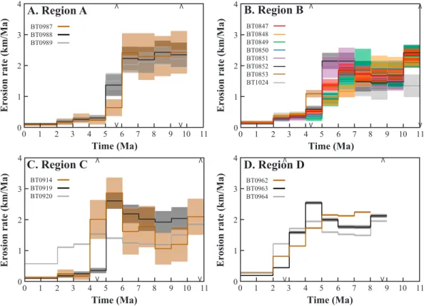
Despite some sample-to-sample variations in derived exhumation rates for any specific time step, the bestfit models for most samples indicate exhumation rates (interpreted here as erosion rates) decreased between MsAr closure (circa 12.3–7.9 Ma) and ApHe closure (circa 6.5–2.8 Ma) and remained relatively low until the present. Our results from all regions show a significant decrease in erosion rate circa 6–4 Ma from high rates approximately 2–3 km/Ma to rates as low as approximately 0.1 km/Ma over the Quaternary (Figure 6).
Though we were thoughtful in our sample collection to test model results for sensitivity to landscape position, wefind similar erosion rate histories within low-relief landscapes (i.e., above knickpoints) and in adjacent canyons (i.e., below knickpoints) and importantly no direct evidence of a recent increase in erosion rate associated with the passing of a knickpoint and surface uplift.
Interestingly, our modeling results from across Bhutan are similar to the 2-D modeling results ofCoutand et al.
[2014] from eastern Bhutan where they found a dramatic decrease in exhumation after 6 Ma when rates where as high as 2 km/Ma. This confirms that our 1-D models capture much of the information content from multichronometer data sets regarding regional and temporal patterns in erosion rate. The most dramatic change in our erosion histories generally occurred between the closure of the ZrnHe and ApHe
systems. The importance of this period of cooling is exhibited in the erosion history of BT0920, which did not have dateable apatite, and therefore displays a less dramatic cooling/erosion history.
Figure 7 illustrates the thermal evolution of a sample with an average erosion history from the Bhutan Himalaya (BT0988). The primary function of the thermal-kinematic model was to predict a temperature- time path (Figure 7b) from an imposed velocity history (Figure 7a). However, we also required that acceptable cooling histories yielded an appropriate closure temperature for all three chronometric systems (based on the predicted cooling rate) at or near the observed cooling ages, and cooled to the surface temperature at 0 Ma (Figure 7b). The thermal-kinematic model also tracked particle trajectories such that depth-time paths (Figure 7b), and the local geothermal gradient could be calculated (Figure 7a). In all the bestfit model simulations the erosion rates slowed circa 6–4 Ma. This decrease in erosion rate changed the thermal regime from one dominated by advection (during times of high erosion), to one of conduction (during times of lower erosion). As conduction became the more dominant process, the geothermal gradient decreased and isotherms moved deeper, causing cooling (Figure 7b).
While our explicit modeled erosion rate histories extend from the late Miocene to recent time steps, it is important to note that the youngest thermochronometric dates in the Bhutan Himalaya are pre- Quaternary, such that neither our models nor those ofCoutand et al. [2014] yield detailed information regarding the potential for variability in Pliocene and Quaternary erosion rates. In our numerical experiments as well as others recently published by Coutand et al. [2014], the only quantitative constraint on erosion rates subsequent to ApHe closure is that the samples must have cooled to surface temperatures in no more than the elapsed time since ApHe closure. This constrains the mean erosion rate, or total exhumation since the late Miocene or Pliocene, depending on location but offers no constraint on variations in erosion rate over this interval. Fortunately, the best fit erosion rate histories place constraints on the overburden thickness of samples at anytime in the history. Effectively, the depth of a sample at a given time is the integral of the erosion rate history curve at that time.
Figure 6.Erosion rate histories from 1-D thermal-kinematic modeling. Bold solid lines show mean histories. Transparent envelopes show two standard errors on the mean history. Erosion rate histories from samples located in Regions (a) A, (b) B, (c) C, and (d) D. See Figure 4 for sample and region locations and thermochronometric cooling ages used in the models. Arrows mark the extent of cooling ages and the associated one standard deviation uncertainties of each region.
Figure 8 shows the mean overburden thicknesses during the erosion histories of Regions A–D. The maximum overburden thickness at the time of ApHe cooling ages, circa 5 Ma for Regions A–C and circa 3 Ma for Region D, places a constraint on the possible total amount of erosion after our youngest thermochronometric data.
In Table 4 we have constructed a simple matrix to evaluate the plausibility of various changes in recent erosion rates post 3 Ma. For a change in erosion history to be plausible we require that the resultant eroded thickness not exceed our maximum eroded thickness values from Regions A–C (approximately 1.7 km) and Region D (approximately 1.8 km) after the closure of the ApHe system (Figure 8). In cases where this value is exceeded, the observed ApHe cooling ages would have been eroded from the surface and therefore are not plausible. The results suggest that a return to the high rates of the mid-Miocene (approximately 2 km/Ma) could have only occurred in the past 750 ka. A return to a more moderate rate of 1 km/Ma could have only occurred in the last 1.75 Ma. (see Figure 8).
We note that Region D records an exhumation path with a similar trend as Regions A–C, but with slightly differing timing and rates (Figures 6 and 8). This could easily be predicted by observing the difference in thermochronometer cooling ages of similar elevations from Regions B and D (Figure 5). The difference between the cooling histories from Regions A–D is likely the result of the sample locations with the range. Region D lies within the largest drainage system in Bhutan, the Kuri Chu basin (Figures 4 and 5).
At this position in the range, the Kuri Chu valley is very wide and deep, which will affect the local geothermal gradient. In addition, the Kuri Chu is coincident with an erosional reentrant in the Main Figure 7.Temperature and depth history of sample BT0988 from Region A. (a) Erosion rate and geothermal gradient histories since 10 Ma. (b) Temperature and depth paths since 10 Ma. Predicted closure temperatures for ApHe, ZrnHe, and MsAr are denoted by red, green, and bluefilled circles, respectively. Afilled brown circle marks the temperature at the surface of the model. Predicted depths of system closure for ApHe, ZrnHe, and MsAr are denoted by red, green, and blue open circles, respectively. Corresponding colored boxes denote the observed cooling age and 1σuncertainties, and possible range of closure temperatures. Solid red, green, and blue lines show the respective predicted closure temperature (Tc) of minerals (which have yet to be exhumed) as a function of time. Dashed colored lines show the predicted depths of the respective closure isotherms (Zc) of minerals (which have yet to be exhumed) as a function of time. Note that the depth of the closure temperature isotherm of each thermochronometric system has increased since circa 6 Ma when erosion rates decreased markedly, and conduction dominated the thermal regime over advection. Also note that the predicted cooling ages are near the limit of the acceptable observed cooling ages due to the uncertainty on the mean history, see Figure 5.
Central Thrust sheet associated with the construction of a N-S trending antiform [McQuarrie et al., 2008].
Such local tectonic activity could have also influenced the thermal/erosional history of Region D.
However, we again emphasize that the most robust signal within all of our data is a regional long-term reduction in erosion rates circa 6–4 Ma.
Figure 8.Mean overburden histories for Regions A–D. Grey envelopes represent 2 standard errors on the mean path. Filled white circles denote inflection points when erosion rates begin to decrease in each region. Open black circles denote the mean ApHe cooling ages. Open and closed circles are roughly coincident for Regions A and C. Dotted black line and numbers illustrate the possible erosion histories based on the maximum erosion since the closure of the youngest thermochronometer (ApHe) and assuming erosion rates of 2, 1, and 0.5 km/Ma.
Table 4. Possible Erosion Histories Post 3 Maa
Time of Change (Ma)
Erosion Rate (km/Ma) 0.50 0.75 1.00 1.25 1.50 1.75 2.00 2.25 2.50 2.75 3.00
3.00 1.50 2.25 3.00 3.75 4.50 5.25 6.00 6.75 7.50 8.25 9.00
2.75 1.38 2.06 2.75 3.44 4.13 4.81 5.50 6.19 6.88 7.56 8.25
2.50 1.25 1.88 2.50 3.13 3.75 4.38 5.00 5.63 6.25 6.88 7.50
2.25 1.13 1.69 2.25 2.81 3.38 3.94 4.50 5.06 5.63 6.19 6.75
2.00 1.00 1.50 2.00 2.50 3.00 3.50 4.00 4.50 5.00 5.50 6.00
1.75 0.88 1.31 1.75 2.19 2.63 3.06 3.50 3.94 4.38 4.81 5.25
1.50 0.75 1.13 1.50 1.88 2.25 2.63 3.00 3.38 3.75 4.13 4.50
1.25 0.63 0.94 1.25 1.56 1.88 2.19 2.50 2.81 3.13 3.44 3.75
1.00 0.50 0.75 1.00 1.25 1.50 1.75 2.00 2.25 2.50 2.75 3.00
0.75 0.38 0.56 0.75 0.94 1.13 1.31 1.50 1.69 1.88 2.06 2.25
0.50 0.25 0.38 0.50 0.63 0.75 0.88 1.00 1.13 1.25 1.38 1.50
aInterior cells are values of total eroded thickness (km) given the time since a possible change in erosion rate (columns) and a possible increased erosion rate (rows). Bold totals denote plausible eroded thicknesses, and therefore plausible changes in erosion rate and time, that are lower than the maximum possible eroded thickness from Regions A–C since 5 Ma (1.68 km). Underlined totals denote plausible eroded thicknesses, and therefore plausible changes in erosion rate and time, that are lower than the maximum possible eroded thickness from Region D since 3 Ma (1.81 km). Italicized totals are too high to preserve observed ApHe cooling ages.
6. Discussion
6.1. Constraining Surface Uplift in Bhutan
Both physical [e.g.,Bonnet and Crave, 2003] and numerical [e.g.,Whipple and Tucker, 1999;Whipple, 2001]
models of landscape evolution demonstrate that during the production of surface uplift, erosion rates within a landscape only increase once a knickpoint in afluvial system has moved through the landscape, since changingfluvial dynamics is the agent of restoring a landscape to equilibrium (Figure 3). As such, landscapes upstream from migrating knickpoints (Regions A and C) cannot be used to accurately test whether the Tectonic Rejuvenation or Climate Hypothesis has created the surface uplift observed in Bhutan. However, models of landscape evolution demonstrate that canyons downstream of migrating knickpoints should currently be eroding at a rate much faster that the uplifted surfaces (Figure 3), yet cooling histories from the incised canyons (Region B and Region D) do not record this increase in erosion associated with either hypothesis. This suggests that the increase is young and that not enough erosion has occurred to exhume thermochronometers that record the landscape evolution (since less than 2 km of incision has occurred since the time of change; see Figure 8). Instead, our cooling histories demonstrate that erosion rates decreased in a sustained manner and thus provide strong evidence for the Tectonic Decline Hypothesis over the Climate Hypothesis in Bhutan. The 6–4 Ma decrease in erosion rates recorded across Bhutan, including in samples from the low-relief surfaces (Regions A and C), is not related to the change in forcing factors that has created the major north migrating knickpoints and surface uplift, but instead this reduction in erosion rates points to an older event that likely caused relief reduction.
Our topographic analysis also shows that low-relief landscapes are present to the west of the proposed Shillong Plateau rain shadow limits approximately 90°E. Because of the similarity in location and form of the low-relief landscapes (Figures 1 and 2), we prefer a common formation mechanism for all of these surfaces. Furthermore, we suggest that a reduction in erosion rate in western Bhutan, which is outside of the Shillong Plateau rain shadow, shows that the observed slowing could not have been related to the rain shadow. In light of this, a widespread tectonic mechanism better explains the surface uplift observed in Bhutan. This implies a need for a recent pulse of increased rock uplift rates at the front of the range or middle latitudes of the Eastern Himalaya, and thus the need for a hybrid hypothesis combining the Tectonic Decline and Tectonic Rejuvenation hypotheses sequentially.
While mean erosion rates over most of Bhutan were around 0.1–0.3 km/Ma over the past 5 Ma, an erosion rate increase in recent times is possible. Due to the relatively old ApHe cooling ages (circa 5 Ma) observed at the surface today and the low amounts of recent erosion that they permit, wefind that it is unlikely that a tectonic mechanism of surface uplift is much older that 1.75 Ma, as this is the maximum duration at which rates approximately 1 km/Ma are permitted by our thermochronometric data. Furthermore, cooling histories from Region D show that a recent increase in erosion rate, if spatially uniform, must be younger than 3 Ma, since ApHe chronometers of this age still record decreasing erosion rates. Since there has not been enough incision around the low-relief landscapes (<2 km) to exhume young thermochronometers (<2 Ma), another quantitative chronometer capable of measuring more recent changes (e.g., cosmogenic nuclide techniques) will be required to better constrain the timing of surface uplift in Bhutan.
6.2. Coupled Tectonic Histories of the Eastern Himalaya and Shillong Plateau
AsCoutand et al. [2014] did before us, we interpret the modeled decrease in cooling/erosion rates circa 6–4 Ma as an indication of decreased shortening in the eastern Himalaya related to a N-S broadening of the region of India-Eurasia shortening to include the Shillong Plateau. Conversely,Long et al. [2012] used geochronometric and thermochronometric data to suggest a similar reduction in 1-D cooling rates in eastern Bhutan as rocks were transported over ramp/flat geometries of the basal thrust fault. However, we find it is highly unlikely that ramp/flat geometries could be responsible for the changes in cooling rates recorded by any of our samples. Based on the existing data from thermochronometric inversions [Coutand et al., 2014], and balanced cross sections [Long et al., 2011, 2012; Tobgay et al., 2012; McQuarrie et al., 2014], the rocks from which we have measured cooling histories have not experienced a transition across a major ramp, and as such we do not expect a significant change in their trajectory toward the surface over their recorded cooling history. In this way we have tried to avoid issues of spatial variability in shortening, rock uplift, and erosion rates associated with geologic structures, to focus on the temporal variability of deformation within the range.
While our easternmost sampling area, Region D, records younger ages and slightly higher erosion rates for longer time periods than western and central regions (Regions A–C), the decreasing trend in erosion rates from Region D and other regions is similar overall. We attribute the distinctive thermal history of Region D to local variability in geothermal gradient or the affects of the Kuri Chu antiform, not to an E-W structural dichotomy in Bhutan associated with the Shillong Plateau fault activity. Simply taking the absolute cooling ages at face value is misleading when considering an E-W structural dichotomy. In fact, such an over simplified hypothesis would suggest the younger ages observed in eastern Bhutan reveal the opposite findings of Coutand et al. [2014], in which eastern Bhutan was interpreted to be more recently active than western Bhutan. Based on thefindings from our thermal-kinematic models and the continuity of topographic indicators, the simplest and most robust interpretation of the thermochronometric data is that all of the Bhutan Himalaya experienced a reduction in erosion rate circa 6–4 Ma and not only those regions directly north of the Shillong Plateau (i.e., east of 90°E). This implies that the region of the eastern Himalaya over which a reduction in shortening rate after the middle Miocene is larger than previously assumed. In particular, this reduction must have included areas west of 90°E (e.g., western Bhutan and Sikkim), an idea supported by the observations ofClark and Bilham[2008], which suggest Shillong Plateau structures have affected surface deposits approximately 88°E. Indeed, the geodetic data presented byVernant et al. [2014] led those authors to suggest essentially the same timing for a dramatic reduction in fault slip rates in western Bhutan as consequence of deformational activity in the Shillong Plateau.
Coutand et al. [2014] interpreted significantly different exhumation histories for thermochronometric data from eastern and western Bhutan based on complex, 2-D thermal-kinematic models. While our interpretations are based on simpler, 1-D models, our inferred exhumation history for eastern Bhutan is quite similar to that of Coutand et al. [2014], underscoring our assertion that 1-D modeling frequently provides comparable tectonic insights. Collectively, our results and those ofCoutand et al. [2014] support reduced late Cenozoic erosion rates in eastern Bhutan. However, unlike those authors, we do not see evidence for a distinctive exhumation history for western Bhutan in our modeling results. Upon inspection, the eastern and western data sets modeled byCoutand et al. [2014] have similar apparent age ranges for the same thermochronometers, and we infer that their interpretation of a different exhumation history for the east as compared to the west derives from their construction of two very different structural models for the orogenic wedge in the east and the west. In fact, cooling age data presented by Coutand et al. [2014] from western Bhutan display an erosion history similar to the new data presented here when inverted with our simpler 1-D thermal-kinematic model (see Figure S2). Unfortunately, we were unable to use their entire thermochronometric data set with our specific thermal-kinematic model setup because our approach requires more spatially constrained data sets obtained using specific thermochronometers with no inverted cooling age/closure temperature data.
We note also thatLong et al. [2012] andMcQuarrie et al. [2014] proposed a reduction in exhumation rates through time in eastern and western Bhutan based on their own 1-D modeling studies, which were tied to interpretations of the structural evolution of the orogenic wedge based on structural observations. While those authors suggested that the decline likely occurred circa 10–9 Ma, and was related to a repartitioning of deformation related to the rise and expansion of the Tibetan and Shilong plateaus to the north and south, respectively, ourfindings suggest a slightly more recent, Miocene-Pliocene decline prior to a late stage of rejuvenation. Again, the thermochronometric data sets they presented did not meet our criteria for modeling, and thus could not be incorporated into our study. However, we infer that the detailed differences between their conclusions and ours reflects a reliance by them on specific assumptions regarding the evolution of structural geometries over time.
In addition to the late Miocene decline in tectonically driven exhumation, another geologic event/process is required to create the widespread surface uplift recorded in Bhutan. The existence of perched low-relief surfaces to the west of the spatial limits of the Shillong Plateau rain shadow is inconsistent with the hypothesis that a reduction in orographic precipitation led to the transient landscapes. Unfortunately, because the orographic rain shadow of the Shillong Plateau may have initiated after 4–3 Ma [Biswas et al., 2007], and few of the existing thermochronometric dates for Bhutan are younger than 4–3 Ma, we were not able to adequately test whether erosion rates responded after the rain shadow may have set in or how the erosion rates might have adjusted over time using thermochronometric data alone.