on Complex Magnetic Structures in Magnetoelectric Materials
Inaugural-Dissertation
zur
Erlangung des Doktorgrades
der Mathematisch-Naturwissenschaftlichen Fakult¨at der Universit¨at zu K¨oln
vorgelegt von
Simon Holbein
aus Leinefelde
Vorsitzender
der Pr¨ ufungskommission: Prof. Dr. Simon Trebst
Fred Vargas [1, p. 17]
1. Motivation 9 2. Magnetoelectric and multiferroic materials 11
2.1. The magnetoelectric effect . . . . 12
2.2. Multiferroic materials . . . . 13
2.2.1. Classification of multiferroics . . . . 15
2.2.2. Ferroelectricity in spiral magnets . . . . 16
2.2.3. Electromagnons: hybridized excitations . . . . 18
3. Neutron scattering techniques 21 3.1. Principal neutron scattering formulas . . . . 22
3.1.1. Nuclear scattering . . . . 23
3.1.2. Magnetic scattering . . . . 24
3.1.3. Inelastic neutron scattering . . . . 26
3.2. Neutron polarimetry . . . . 30
3.2.1. Basic formulas . . . . 30
3.2.2. Experimental techniques . . . . 34
4. Electromagons in TbMnO
337 4.1. Introduction . . . . 38
4.1.1. Crystal and magnetic structure . . . . 38
4.1.2. Multiferroic phase . . . . 40
4.1.3. Application of magnetic fields . . . . 42
4.1.4. Magnetic and magnetoelectric excitations . . . . 43
4.2. Diffuse scattering above the magnetic and multiferroic phase tran- sitions . . . . 44
4.2.1. Antiferromagnetic transition at T
N. . . . 45
4.2.2. Multiferroic transition at T
FE. . . . 53
4.3. Model for magnetic excitations . . . . 57
4.4. Magnetic excitations in the incommensurate phase . . . . 63
4.4.1. Fitting of the magnon dispersion . . . . 64
4.4.2. Comparison to time-of-flight data . . . . 67
4.4.3. Chirality of excitations . . . . 73
4.4.4. Influence of the Tb-subsystem . . . . 78
4.5. Magnetic excitations in commensurate high-field phase phase . . . 81
4.5.1. Zone-center modes in the HF-C phase . . . . 83
4.5.2. Dependency of modes on H
b, T and Q . . . . 87
4.6. Conclusion . . . . 89
5. Magnetic fluctuations in MnWO
491 5.1. Introduction . . . . 92
5.1.1. Crystal and magnetic structure . . . . 92
5.1.2. Multiferroic AF2 phase . . . . 94
5.2. Diffuse magnetic scattering . . . . 98
5.2.1. Sample characterization . . . . 99
5.2.2. Antiferromagnetic transition at T
N3. . . . 101
5.2.3. Multiferroic transition at T
N2. . . . 110
5.2.4. Relaxation times of magnetic fluctuations . . . . 116
5.3. Magnetic excitations in the multiferroic phase . . . . 119
5.4. Conclusion . . . . 123
6. Magnetic phase diagram of NaFe(WO
4)
2125 6.1. Introduction . . . . 126
6.1.1. Crystal and magnetic structure . . . . 126
6.1.2. Magnetic phase diagram and dielectric measurements . . . 127
6.2. Neutron diffraction in the zero field phase . . . . 130
6.2.1. Temperature dependence of magnetic order . . . . 130
6.2.2. Magnetic propagation vector . . . . 133
6.2.3. Diffuse magnetic scattering . . . . 134
6.3. Symmetry analysis . . . . 136
6.4. Structure determination of the zero-field phase . . . . 137
6.5. Neutron diffraction of high-field phases . . . . 142
6.5.1. Magnetic field dependence of the propagation vector . . . 142
6.5.2. Commensurate magnetic structures . . . . 143
6.6. Conclusion . . . . 146
7. Ni
0.42Mn
0.58TiO
3, a magnetoelectric spin glass 149 7.1. Introduction . . . . 150
7.1.1. The Ni
xMn
1-xTiO
3system . . . . 150
7.1.2. Magnetoelectric effect in the spin-glass phase . . . . 154
7.2. Magnetic properties of the spin-glass phase . . . . 155
7.2.1. Sample characterization . . . . 156
7.2.2. Temperature dependence of magnetic reflections . . . . 157
7.2.3. Q -dependence of magnetic reflections . . . . 160
7.3. Polarized neutron diffraction . . . . 165
7.3.1. Temperature dependence and polarization of ordered mag- netic moments . . . . 166
7.3.2. Influence of magnetic and electric fields . . . . 170
7.4. Magnetic excitations in the spin-glass phase . . . . 174
7.4.1. Zone center excitations . . . . 174
7.4.2. Q -dependence of magnetic excitations . . . . 175 7.4.3. Spin wave model . . . . 181 7.5. Conclusion . . . . 186
8. Summary 187
A. Unit conversion 191
B. SpinW code for TbMnO
3193
C. Supplemental data for Ni
0.42Mn
0.58TiO
3195 C.1. Field dependence of magnetic scattering components . . . . 195 C.2. Magnetic excitations . . . . 198
Bibliography 201
Glossary 223
Abstract 227
Kurzzusammenfassung 229
Danksagung 231
List of Publications 233
Offizielle Erkl¨ arung 235
Motivation
In order to increase the functionality of technical devices, there is ongoing re- search for materials with sophisticated properties. Especially the coupling between electric and magnetic properties in a material, known as the magnetoelectric effect, has the potential to improve today’s technology [3]. The effect was predicted already in the 19th century [2] but its application was hindered in the last century by the low number of available materials and the weakness of the effect [4]. The recent discovery of spin-induced ferroelectricity in TbMnO
3showed that frustrated magnets are ideal systems to develop a giant coupling between magnetic and electric order [5].
In magnetic oxides, frustration can arise due to competing magnetic exchanges and anisotropies. Common examples are systems with geometric frustration or competing nearest- and next-nearest neighbor exchanges [6, p. 173ff]. The frustra- tion destabilizes the magnetic order which can subsequently be modulated even by the intrinsically weak magnetoelectric effect [7]. As a result, these systems show spectacular cross-coupling effects, such as magnetically induced polarization flops [8] and giant magneto-capacitance [9].
Systems in which a complex magnetic structure directly induces a ferroelectric po- larization generated great interest [10]. These multiferroic systems with coexisting antiferromagnetic and electric order develop per definition a strong coupling of both orders. Neutron scattering is an experimental technique which is perfectly adapted to study antiferromagnetic materials. It has been a valuable tool to understand the microscopic properties of these interesting materials [11, 12, 13]. The aim of current research is to find novel multiferroic and magnetoelectric materials and to understand the various underlying microscopic origins that can lead to such effects [14].
In this thesis, experimental data on four different transition-metal oxides was
gathered and evaluated. Their magnetic properties were investigated by neutron
scattering on single crystalline samples. In order to study the magnetic structure, the critical behaviour and the dynamics of the systems, several different scattering techniques were applied. The observations contributed to a better understanding of the underlying physics. This work contains two introductory and four experimental chapters which are organized as follows:
Chapter 2 introduces the recent developments concerning the magnetoelectric effect and multiferroic materials. The focus is on multiferroics whose ferroelectric polarization is induced by a spin-spiral structure via the inverse Dzyaloshinskii- Moriya effect [15, 16], and on the first observations of electromagnons: hybridized phonon-magnon excitations.
The experimental technique of neutron scattering is presented in Chapter 3. The basics of nuclear and magnetic scattering are briefly summarized, followed by an overview of the use of neutron polarization analysis. The different experimental techniques applied in this work are introduced.
TbMnO
3, which is discussed in Chapter 4, is a prototype material for spin-induced multiferroics. In this material, the spiral order of Mn-moments accounts for the induced ferroelectricity [5]. The sequence of magnetic phase transitions and the correlation of the magnetic moments were investigated. The spin dynamics in the multiferroic phase were studied in detail and a spin-wave model was developed which can describe the full magnon dispersion. In addition, the magnetic excitation spectrum in the multiferroic high-field phase is analyzed and the influence of the rare-earth ion on the excitation spectrum is discussed.
Another prototype multiferroic is MnWO
4, which is presented in Chapter 5.
A complex spin-spiral of Mn-moments induces an electric polarization in this system [17]. The properties of the sequence of magnetic phase transitions were investigated in detail. The use of polarized neutrons in combination with applied magnetic fields allowed to observe ferroelectric fluctuations in the dielectric phase.
Furthermore, the excitation spectrum in the multiferroic phase is presented.
Chapter 6 presents a comprehensive study of the magnetic phase diagram of NaFe(WO
4)
2. The double tungstate is isostructural to MnWO
4and it could be demonstrated in this work that the system develops a similar spin-spiral structure.
In a magnetic field applied along ~b, the structure transforms into a collinear antiferromagnetic structure.
Finally, Chapter 7 presents studies on the ilmenite Ni
0.42Mn
0.58TiO
3. In this
material, the linear magnetoelectric effect was observed in the absence of a long-
range magnetic order [18]. It could be shown, that two competing orders are
coexistent in the spin-glass phase and that the antiferromagnetic domains can be
controlled by the application of crossed magnetic and electric fields. Furthermore,
the magnetic excitations in the spin-glass phase were investigated and compared
to spin-wave simulations.
Magnetoelectric and multiferroic materials
Figure 2.1.:
Classification of mag- netic and electric properties in in- sulating oxides. Rounded squares correspond to materials being elec- trically polarizable (PE), magneti- cally polarizable (PM), ferroelectric (FE) and ferromagnetic (FM). In-
spired from Ref. [19].
The fundamentals of electricity and magnetism, and in particular their interaction, are stated in Maxwell’s equations from 1865 [20]. In condensed matter, these two phenomena are separated due to their distinct ori- gin: electric charges on one hand, and spins on the other hand. While there are many materials in which one of these effects can be observed, materials with coexisting or coupled order are rare.
Figure 2.1 sketches the distribution of electric (red) and magnetic (green) properties in the material class of in- sulating oxides, indicating regions of polarizability and ferroic order. Multiferroic materials are materials at the intersection of ferromagnetism and ferroelectricity.
Materials showing a coupling of magnetism and elec- tric properties, i.e. the magnetoelectric effect, which is indicated by a white region, span over four different intersections.
In this chapter, an overview is given of the magneto- electric effect and the class of multiferroic materials.
The focus is on the materials investigated in this work,
which positions are indicated in Fig. 2.1 as a star (TbMnO
3and MnWO
4) and a
triangle (Ni
0.42Mn
0.58TiO
3).
2.1. The magnetoelectric effect
The term ”magnetoelectric (ME) effect” denotes in general the coupling between magnetic and electric properties in matter. In times of a booming digital industry with increasing demand for electronic storage and computing capacity, this effect opens possibilities for novel applications [21]. The interest in this field of research increased enormously since the beginning of the new century [7], revitalized, among others, by the observation of a giant ME effect in TbMnO
3in 2003 by Kimura et al. [5]. A detailed overview of the recent revival of the ME effect is given in Ref. [7].
The first reference of the ME effect can be traced back to Pierre Curie in 1894, who pointed out the possibility of such an effect on the basis of symmetry considera- tions [2]. But the effect was not experimentally observed before 1960, when Astrov reported a linear ME coupling in Cr
2O
3[22], which has been theoretically predicted by Dzyaloshinskii [23]. Since then, a variety of materials has been discovered, spanning over the complete region denoted in Fig. 2.1.
Following the phenomenological approach by Landau, the ME effect can be de- scribed by the free energy F ( E, ~ ~ H) of a material [24]. Differentiation of F with respect to E ~ or H ~ leads to the polarization and magnetization:
P
i( E, ~ ~ H) = − ∂F
∂E
i= P
is+
0ijE
j+ α
ijH
j+ 1
2 β
ijkH
jH
k+ γ
ijkH
iE
j+ ... (2.1) M
i( E, ~ ~ H) = − ∂F
∂H
i= M
is+ µ
0µ
ijH
j+ α
ijE
i+ β
ijkE
iH
j+ 1
2 γ
ijkE
jE
k+ ... (2.2) P ~
sand M ~
sare the spontaneous polarization and magnetization,
ijis the electric and µ
ijthe magnetic susceptibility and
0and µ
0are the electric and magnetic constants. The tensor susceptibility α
ijdescribes the linear magnetoelectric effect, i.e. the induction of an electric polarization by a magnetic field and of a mag- netization by an electric field. The linear effect is accompanied by higher order terms, characterized by the tensors β
ijk(bilinear ME effect) and γ
ijk(quadratic ME effect). In the following, we will focus on the linear effect, omitting higher order terms.
The linear ME effect is only observed in few materials, and its limitation can be
understood by a symmetry analysis. Electric and magnetic polarization behave
differently on time reversal and spatial inversion operations. The electric polar-
ization, given by an electric dipole, is invariant under time reversal and changes
its sign under spatial inversion. The case for the magnetization can be visualized
when expressing the magnetic moment by small current loops. These are invariant
under spacial inversion, but change their current direction under time reversal.
This implies, that the linear ME tensor α
ijcan only be non-zero for a material which simultaneously breaks both time reversal and spacial inversion.
The symmetry constraints given above limit the number of magnetic groups in which the linear ME effect is possible. One can deduce, that the effect is excluded for all dia- and paramagnets, as their magnetic space groups contain the time reversal operator 1
0. Furthermore, the magnetic space group cannot posses a center of symmetry ¯ 1. Overall there are 58 magnetic points groups, which allow for the linear magnetoelectric effect, summarized in Ref. [25, p. 138]. The magnetic point group of the system determines the shape of the ME tensor, e.g. the existence of diagonal and off-diagonal terms.
A detailed study of the microscopic origin of the magnetoelectric effect in ordered magnetic compounds was published in Ref. [26]. These are crucial in order to understand the strength of the effect and to be able to design materials suiting technical applications. In general, the effect can be described as a perturbation of an external field, modulating a microscopic exchange or anisotropy parameter. As an example, the electric field can move ions relative to its ligands, modulating the ions anisotropy or exchange path. The relevant interactions discussed to induce the ME effect are (in order of strength): the single-ion anisotropy, the symmetric superexchange, the antisymmetric superexchange, dipolar interactions and the Zeeman effect [26]. Technical applications based on the ME effect strongly depend on the strength of the effect. In the compounds that are known until now, the effect is relatively weak. It could be shown that an important limitation exists for the size of the ME tensor [27]:
α
2ij<
iiµ
jj. (2.3) This upper boundary of α
ijis given by the geometric mean of the materials mag- netic and electric susceptibilities. The chances to observe a strong ME coupling are thus increased for materials which develop strong ferroelectric and magnetic order.
2.2. Multiferroic materials
The limitation of the linear magnetoelectric effect, given by Eq. 2.3, shows that
materials with simultaneous ferroelectric and magnetic order are best suited to
exhibit strong ME effects. The term multiferroic used by Schmid in Ref. [28] is
now widely recognized for this group of materials (ferroelectromagnets was also
used in earlier publications [29]). In its initial formulation, this term is used to
state the coexistence of at least two types of ferroic ordering, i.e. ferroelectricity,
ferromagnetism and ferroelasticity. In a broader context, also ferri- and antifer- romagnetic order along with ferrotoroidal order are included in the term. The multiferroic materials investigated in this work, TbMnO
3and MnWO
4, show the coexistence of ferroelectric polarization and antiferromagnetic order.
It is indicated in Figure 2.1 that the magnetoelectric effect is not necessary a property of a multiferroic material. This is for example the case for the widely studied room-temperature multiferroics BiFeO
3and BiMnO
3. It can be explained by the distinct microscopic origin of both ordering types in these materials [10].
The first multiferroic material, in which both ferroic orderings were observed simultaneously in the absence of magnetic and electric field, was Ni
3B
7O
13I in 1966 [30]. There are two aspects that explain the difficulty of having magnetism and ferroelectricity together in the same phase. On one hand, the system has to obey specific symmetry restrictions, similar to the ME effect. The space group of the system must simultaneously break time reversal and spacial inversion symmetry, in order to allow for both ordering types (see Ref. [31] for a comprehensive discussion of symmetry aspects for multiferroic materials).
On the other hand, magnetic order and ferroelectricity have a distinct microscopic origin. Most ferroelectric materials are transition-metal oxides with perovskite structure, where the metal ion is in the center of an oxygen octahedron. For metals with an empty d-shell, a covalent bonding with an oxygen atom is often favored in order to reduce binding energy [32]. The metal ion then shifts toward an oxygen atom which induces an electric dipole moment. In materials with such an electron configuration, it is not possible to develop a magnetization because all electron shells are either full or empty and the electron spins cancel out each other . Magnetic ordering is a common feature of perovskite transition-metal oxides and arises in general from the intrinsic spin of localized electrons. In contrast to ferroelectricity, it requires metal ions with partially filled shells. The outcome of this incompatibility of ferroelectricity and ferromagnetism is often referred to as d
0-rule [4].
In the following, we will describe different types of multiferroic materials, with a strong focus on systems in which a spiral magnetic structure directly induces ferroelectric polarization. Two chapters in this work are dedicated to materials belonging to this group, namely TbMnO
3and MnWO
4. A more detailed distribu- tion of multiferroic materials of all types can be found in References [33] and [6, p.
288ff].
2.2.1. Classification of multiferroics
The multiferroic materials can generally be classified into two groups, following the approach by Khomskii [34]
a. The first group, called type-I multiferroics, contains materials in which magnetism and ferroelectricity have a distinct origin. BiFeO
3is a famous example of this group, with a multiferroic phase at room temperature.
In this case, the two ordering types can be attributed to different ions, yielding a weak ME interaction [36].
The second group, type-II multiferroics, covers materials in which one type of ordering directly induces the other, leading to an intrinsically strong ME coupling.
TbMnO
3was the first type-II material to be found in 2003 in the group of Kimura [5]. Magnetic and electric order are coexistent and their origins are coupled. The magnetically ordered state induces an electric polarization and thus causes ferroelectricity.
These multiferroics of spin origin are known to exhibit strong magnetoelectric effects. This renders this class of materials interesting to study for the reason of both fundamental physics and technical applications in spin-related electronics [37].
There exist many comprehensive reviews about the spin-induced ferroelectrics, among them References [14] and [38].
Common for all multiferroics of spin origin is the fact that the magnetic structure breaks the inversion symmetry, which is a necessary condition for the development of a spontaneous ferroelectric polarization. The major underlying microscopic mechanism for this effect, which were study up to today, can be classified belonging to one of three models: (a) exchange striction model, (b) inverse Dzyaloshinskii- Moriya (DM) model and (c) spin-dependent p-d hybridization model [14]. We will shortly present the main idea of the models (a) and (c) and focus in the next section on the inverse DM model (b).
The ferroelectricity in model (a) can be attributed to the symmetric spin exchange interaction ˆ J
ijbetween neighboring spins, S ~
iand S ~
j, and is of the form
(a) P ~
ij∝ J ˆ
ij( S ~
i· S ~
j) . (2.4) The interaction can induce striction along a specific crystallographic direction, yield- ing a net ferroelectric displacement of ions. A famous example is the commensurate spin chain ↑↑↓↓ along an alternating lattice with A and B-sites. This structure breaks the inversion symmetry. A modulation of the strength of antiferromagnetic (AFM) and ferromagnetic (FM) exchange leads to a variation of bond-lengths, inducting oriented electric dipoles [6, p. 297]. This can occur in systems with magnetic chains of alternating valences, which is the case for Ca
3CoMnO
6[39].
aArtificial multi-layer compounds are excluded from this consideration. The interested reader is referred to a dedicated review article such as Ref. [35].
There are also single-valence systems, where the FM and AFM interactions are modulated by the bond-angle of the superexchange. An example is the E-type magnetic phase of the RMnO
3series, where R stands for a rare-earth ion [40].
The exchange-striction model is independent of the spin-orbit coupling (SOC) and consequently exceeds in most systems the magnitude of the other models.
The spin-dependent p-d hybridization model is based on the SOC, similar to the inverse DM model. The connecting vector ~ r
ikbetween a spin at site i and its ligand at site k can be modulated by the spin-dependent hybridization [41, 42].
The resulting polarization points along the direction of the bond and is of the form:
(c) P ~
ik∝ ( S ~
i· ~ r
ik)
2~ r
ik. (2.5)
2.2.2. Ferroelectricity in spiral magnets
The inverse DM model (b) explains the appearance of spin-induced electric polar- ization in systems of spiral order. According to Khomskii, most type-II multiferroic materials known by date show this effect [6, p. 293]. A spiral spin order is formed in frustrated magnets, materials in which the magnetic ground state is highly degenerated and thus has a complex magnetic structure. The degeneracy can be due to competing FM and AFM exchange interaction or geometrical properties that forbid simultaneous minimization of the interaction or anisotropy energies.
The competition of interactions leads to the development of a complex long-range ordering of magnetic spins, which can be commensurate or incommensurate relative to the crystallographic unit cell.
The induced ferroic displacement in spin-spirals can be related to the relativistic spin-orbit coupling, and is of the form:
(b) P ~
ij∝ ~ r
ij× ( S ~
i× S ~
j) . (2.6) Microscopically this effect was explained in terms of the spin-current [15], which implies a purely electronic displacement, and in terms of the inverse DM in- teraction [16], yielding a displacement of ions. This expression was also de- rived phenomenological from the thermodynamic potential of spiral magnets by Mostovoy [43]. The DM interaction (also referred to as antisymmetric or anisotropic exchange) results from a relativistic correction of the superexchange interaction and is of the form D ~
ij( S ~
i× S ~
j) [23, 44]. The situation is sketched in Figure 2.2.
Two spins S ~ at sites i and i interact via an oxygen ion. When the bridging ion
is displaced from the equilibrium position, the system can reduce its energy by a
canting of spins. If the neighboring spins are already canted, which is generally
Figure 2.2:
Sketch of antisymmetric superex- change between two spins
S~iand
S~jwith con- necting vector
~rijvia a bridging oxygen ion. The Dzyaloshinskii-Moriya-vector follows the condition
D~ij=
~rij ×~x.the case for spin-spirals, then the inverse effect can arise, namely a displacement of oxygen ions away from the equilibrium position [16].
The development of a net ferroelectric polarization strongly depends on the form of the spin spiral. While in a helical spiral, where the spins rotate in a plane perpendicular to the propagation vector, the displacements macroscopically cancel out to zero, in a cycloid spiral, with spins rotating in a plane parallel to the propagation direction, the displacements occur along the same direction resulting in a net electric polarization [34].
Prominent examples which belong to this subgroup of type-II multiferroics, are TbMnO
3[5], Ni
2V
3O
8[45] and MnWO
4[17, 46, 47]. In all these compounds, the development of a spin-spiral of cycloid type coincides directly with the onset of a ferroelectric polarization. The close coupling leads to colossal magnetoelectric effects, e.g. it was shown that the electric polarization can be suppressed or flopped by applied magnetic fields. For example in TbMnO
3, the induced ferroelectric polarization flops from P
cto P
ain magnetic fields parallel to ~a and ~b [8]. The flop coincides with a flop of the spin spiral [48]. Polarized neutron analysis turned out to be a valuable tool to prove the coupling of spin-spiral and polarization. For example it could be demonstrated, that an applied electric field can align and flip the spiral domains [49, 50] and the hysteresis and switching behaviour of the spin-spiral could be investigated [51, 52].
It was mentioned before, that the induced ferroelectricity in this type of multifer- roics is based on the spin-orbit coupling. It can be written as H
SO= λ~ L · S ~ in the LS scheme, which applies for most transition-metal oxides [53, p. 35], with L ~ being the orbital momentum. The spin-orbit constant is proportional to the atomic number
b. In transition-metals with 3d electrons, SOC is generally weak and enters the Hamiltonian of the systems only as perturbation. Nevertheless, it can play a significant role in frustrated system leading to the fascinating multiferroic phases, as discussed above.
bFor hydrogen-like atomsλ∝Z4 is valid. The dependency is more complex for solids and is closer toλ∝Z2 [53, p. 35].
Figure 2.3:
Sketch of zone center magnon modes of a cycloid spin spiral propagating along
~b.The static spin structure is marked by gray, and the lo- cal fluctuations by colored arrows. The modes can be separated in a rotation around the normal vector of the cycloid
~a(top, phason mode), around the propaga- tion direction
~bdirection (middle, cycloid mode) and around
~c, the vector in thecycloid plane perpendicular to
~b(bottom, helical mode). The axis vectors show the oscillation of the spin vector products
S~i×S~j.
2.2.3. Electromagnons: hybridized excitations
The close coupling of magnetic and electric properties in the spin-induced mul- tiferroics also results in a new type of hybridized magnon-phonon modes, often referred to as electromagnons. Katsura et al. developed a theoretical model for the excitation spectrum in the case of a cycloid spin-spiral [54]. Following the inter- pretation by Senff et al. [12], Figure 2.3 sketches the different expected collective spin excitations at the zone center for a bc spin spiral propagating along ~b. From top to bottom, we can distinguish three different excitations, corresponding to (i) a rotation of spins around the normal vector of the cycloid ~a, the phason mode, (ii) a rotation around the propagation vector ~b, of the cycloid, the cycloid mode, and (iii) along the vector ~c, which is perpendicular to the normal vector and the propagation vector of the cycloid, the helical mode. The same expressions are used to distinguish the different modes as in Ref. [55].
Based on the DM mechanism, represented by Eq. 2.6, it is possible to attribute an electric character to the zone center modes. The direction of induced electric polarization is dependent on the cross product of neighboring spins, the vector chirality:
~ v
chiral= S ~
i× S ~
j. (2.7)
The modulation of ~ v
chiralfor the three modes is presented in Fig. 2.3 by colored
vectors in the coordinate system. While the phason mode has no influence on ~ v
chiral,
the cycloid mode (middle) rotates ~ v
chiralalong ~b and the helical mode (bottom)
rotates ~ v
chiralaround ~c. From Equation 2.6, we can deduce that only the cycloid
mode modulates the direction of the ferroelectric polarization, which results in
an oscillation of P ~ along ~a. The magnetic cycloid mode should thus be excited
by an applied electric field. This mode is the Goldstone mode of the ferroelectric transition and should possess zero energy [54, 56].
The first experimental observations of electromagnon modes in a multiferroic material was reported by Pimenov et al. [57]. By using infrared (IR) spectroscopy they observed two modes in TbMnO
3, which were magnetically active and could be excited by an electric field. Later IR studies revealed two additional modes at higher energies in the same compound [58]. The lower mode could be identified by inelastic neutron scattering (INS) with polarization analysis to correspond to an out-of-plane excitation at the magnetic zone center [12]. The assumption, that this mode corresponds to the electromagnon of the DM mechanism could be manifested by successive IR [59, 60] and INS experiments [56, 61], showing that the electromagnon follows the orientation flop induced by magnetic fields. Another electromagnon of DM-origin has been observed in Eu
0.55Y
0.45MnO
3[62].
The electromagnon with the strongest spectral weight, which is observed in TbMnO
3at higher energies, has to arise from a different effect. Several experimental observations in applied field excluded an DM-origin for this mode [59, 63, 64, 65]. In multiferroic RMnO
3, the strongest magnetoelectric mode is always found along ~a, independently of the orientation of the cycloid plane. Vald´ es Aguilar et al. were able to explain this mode based on a modulation of the symmetric exchange [66]. The electric field induces a structural distortion, which is associated with the rotation of the [MnO
6]-octahedra around ~c in RMnO
3. The distortion modulates the FM nearest-neighbor exchanges along ~b, resulting in a rotation of spins. Instead of the DM-electromagnon, which is a zone center mode, the Heisenberg-electromagnon is at a finite momentum transfer ~k = 1 − ~k
incnear the zone boundary [55]. The electromagnon based on Heisenberg exchange can be much stronger than the one of the DM mechanism [66].
Electromagnetic excitations have been observed in a series of spin-induced multi-
ferroics (see Ref. [14] for a review) and were recently observed also in the absence
of spin-driven ferroelectricity, e.g. in CuFeO
2[67]. They enlarge the spectrum of
fascinating effects correlated to the strong magnetoelectric coupling in this group
of materials. Possible applications of this type of excitation, especially in the field
of spintronics, are discussed for example in References [68] and [69]. It was also
suggested to use the multiferroic Goldstone mode in order to deliver electricity
without energy loss and to manipulate domain walls [70].
Neutron scattering techniques
The principal experimental technique applied in this work was coherent neutron scattering on single crystals. There are several advantages of using neutron as projectile, in comparison to X-rays, rendering them most suitable for the study of magnetic structures and excitations. Their weak interaction with matter allows for complex experimental setups, the variation of scattering lengths enables the investigation of light elements and different isotopes, their de-Broglie wavelength can be modulated to be in the range of lattice parameters and most of all, their intrinsic magnetic moment can interact with unpaired electron spins in matter.
The experiments presented in this work were performed at the neutron reactor sources Institut Laue-Langevin (ILL) in Grenoble (France), Laboratoire L´ eon Bril- louin (LLB) in Saclay (France) and Forschungsreaktor M¨ unchen II (FRM II) in Garching (Germany). Different instrumental techniques were applied including magnetic diffraction, inelastic magnetic scattering, neutron spin-echo spectroscopy and neutron polarimetry.
In this chapter, the principal formulas for elastic and inelastic scattering on the crystal and magnetic structure are presented, along with a brief description of the instrumental approaches applied in this work. The focus is on techniques using polarized neutrons, which allows to increase the information obtained from scattering experiments.
For a comprehensive documentation of experimental neutron scattering, the inter-
ested reader is referred to dedicated literature, e.g. by Wills and Carlile [71] or by
Furrer et al. [72].
3.1. Principal neutron scattering formulas
The first observation of antiferromagnetism was achieved by neutron diffraction by Shull and Smart in 1949 [73], shortly after the discovery of the neutron by Chadwick in 1932 [74]. The idea of magnetic neutron scattering originated from Bloch, who pointed out, that the intrinsic magnetic moment of neutron and proton are similar [75]. The scattering technique was extended by Brockhouse and Steward in 1955 in order to also detect inelastic processes on crystal excitations [76]. In the 70 years since then, the flux at the neutron sources was increased and the experimental techniques were perfectionized. The theory of nuclear and magnetic neutron scattering is presented for example in References [77] or [78], from which the formula were taken.
The neutron is a subatomic particle of spin S
n= 1/2 (µ
n≈ −1.91 µ
N, with µ
Nbeing the nuclear magneton), with an average vanishing electronic charge and a rest mass of m
n≈ 1.67 · 10
−27kg. The energy of propagating neutrons is given by E =
12mv
2. It is common to give different equivalent dimensions to describe the energy of neutrons: Energy in meV, Temperature T = E/k
Bin K, wavelength λ = h/mv in ˚ A and wave vector k = 2π/λ in ˚ A
−1. Neutrons with wavelengths in the order of lattice parameters of crystals correspond to a temperature of about 300 K and are denoted as thermal neutrons. A conversion table for several neutron energies is given in Appendix A.
Neutrons are scattered by the nuclei and by the unpaired electrons in the material.
The result is a superposition of nuclear and magnetic contributions, and both have to be taken into account in order to understand the observed data.
The ratio of total scattered neutrons per time I
sand incident neutron flux I
totis denoted as cross section σ
tot= I
s/I
tot. In an experiment, only a part is covered by the detector, given by the double differential cross-section d
2σ/dωdE, within a given solid angle dΩ and an energy interval E to E + dE. In a scattering process, we differ between initial state i and final state f . When the state of the scattering system changes from λ
i→ λ
fand the neutron wave vector and spin state change from (~k
i, σ
i) → (~k
f, σ
f), the differential cross section is given by Fermi’s golden rule:
d
2σ dΩdE
~ki→~kf
= 1 N
k
fk
im 2π ~
2 2X
λiσi
p
λip
σiX
λfσf
h~k
fσ
fλ
f|V |~k
iσ
iλ
0i
2
δ(E + E
λi− E
λf) . (3.1)
In the equation, p
jis the probability to find neutron or the system in the initial state and V is the interaction potential. This is the master formula for neutron scattering and it is valid even without the knowledge of the exact interaction between sample and neutron [78]. It is the basis for all neutron scattering experiments.
3.1.1. Nuclear scattering
Neutrons interact with the nucleus via the strong-force interaction. The efficiency of neutron scattering by a single nucleus is expressed by its scattering length b:
b
2= σ
tot/4π. The strength of the nucleus-neutron interaction depends on the details of the nuclear structure, which cannot be related to the atomic number in a simple way. The value of b can vary greatly between elements of similar atomic number and even between isotopes of the same element.
The wavelength of thermal neutrons is of orders of magnitude higher than the dimension of the nucleus, and the interaction potential of a system of N atoms at positions R ~
lcan be approximated by a delta function:
V
nuc(~ r) = 2π ~
2m
X
l
bδ(~ r − R ~
l) . (3.2)
The proportionality factor b is called neutron scattering length and varies for different elements and isotopes. In a material which is a composition of isotopes, this gives rise to coherent scattering and incoherent scattering. The coherent part shows interference effects and enables to deduce informations about the nuclear structure. The non-interfering incoherent part arises from deviations fo the scattering length relative to the mean value. In the following, we will focus only on coherent scattering.
By inserting V
nucin Equation 3.1, the differential cross section for elastic coherent nuclear scattering can be derived:
dσ dΩ
N,coh
= 8π
3v
0X
~ τ
|F
N( Q)| ~
2· δ( Q ~ − ~ τ) , (3.3)
with the scattering vector Q ~ = ~k
f− ~k
iand the volume of the unit cell v
0. The positions of atoms in a periodic crystal can be expressed as:
R ~
i(t) = R ~
l+ ~ r
j+ ~ u
i(t) . (3.4)
The vector R ~
ldenotes the coordinate of the unit cell, ~ r
jis the equilibrium position
of the atom in the unit cell and ~ u
i(t) is the displacement from the equilibrium
position due to thermal motion. The nuclear structure factor is given by:
F
N( Q) = ~ X
j
b
je
iQ·~~ rje
−Wd(Q)~. (3.5)
The term e
−Wd(Q)~is the Debye-Waller factor, which takes into account the effect of thermal motion of atoms on the interference pattern. The coherent nuclear Bragg scattering can thus be derived from the calculation of the nuclear structure, which takes into account the lattice symmetry, the position of atoms in the unit cell and the different scattering length.
Instrumentation
With the help of Equation 3.3, it is possible to compare experimental observed intensities at nuclear Bragg positions with calculations of F
N( Q) for a given struc- ~ ture. Such experiments are generally performed on powder diffractometers or, when investigating single crystals, on four-circle diffractometers such as the D10 at the ILL [79, p. 38f]. The correct integration of intensity, which is broadened in Q-space due to a ~ Q-dependent instrument resolution and a finite mosaicity of the crystal is a crucial part of the experiment. In addition, extinction effects and absorption can temper the observed intensities and have to be taken into account [80].
The analysis of nuclear scattering intensities determined on D10 has been done using the program FullProf [81]. In addition, a program for MATLAB [82] was written to calculate F
N( Q) for the materials investigated in this work. ~
3.1.2. Magnetic scattering
Magnetic neutron scattering arises from the dipole-dipole interaction between the magnetic moment of neutron and unpaired electrons in matter. The interaction potential of a neutron in spin state ~ σ
Nand propagating electron with momentum
~
p and spin ~ s can be written as follows:
V
mag(~ r) = −γµ
N2µ
B~ σ
N·
"
∇ × ~ s × R ~ R
3!
+ ~ p × R ~
~ R
3#
. (3.6)
The gyromagnetic ratio γ = 1.9132 and the nuclear and Bohr magneton, µ
Nand µ
B, enter the equation. The two terms of V
magin brackets are due to the intrinsic electron spin and the orbital motion of the electron, respectively. V
magis, in contrast to V
nuc, anisotropic due to the axial symmetry of the dipole field. By integrating V
magin the master equation, Eq. 3.1, the elastic and purely magnetic cross-section for an unpolarized neutron beam can be written as follows:
dσ dΩ
M,coh
= 1 N
m8π
3v
0X
~ τM
| F ~
M⊥(~ τ
M)|
2· δ( Q ~ − ~ τ
M) , (3.7)
with N
mbeing the number of magnetic ions and ~ τ
M= ~ τ ± ~k being the reciprocal vector of the magnetic structure. ~k is the propagation vector of the magnetic structure and denotes its periodicity relative to the crystal structure. Finally, the magnetic interacting vector F ~
M⊥is connected to the magnetic structure factor F ~
Mas F ~
M⊥= Q ~ ˆ × F ~
M× Q. Only scattering from electron spins perpendicular to ~ ˆ Q ~ contribute to the magnetic cross section. The magnetic structure factor is given by:
F ~
M( Q) = ~ X
j
f
jM(Q) m ~
je
iQ·~~rje
−Wd(Q)~. (3.8)
f
jMis the magnetic form factor which describes, similarly to the atom form factor, the distribution of magnetic moments in an atom. This leads to a decrease of magnetic intensity at larger Q, whereas the nuclear scattering length is independent of Q. Furthermore, the magnetic cross section is strongly dependent on the direction of the magnetic moments relative to Q, as only the components of the magnetization ~ perpendicular to the scattering vector account for the magnetic cross section.
When the magnetic unit cell has the same size as the lattice unite cell, magnetic reflections are at the same position as the nuclear reflections. In this case, the coherence between neutrons scattered by the nucleus and the magnetic moment is of importance. Only in case of scattering from an unpolarized neutrons beam, where the direction of neutron spins is distributed randomly, interference terms cancel out and the absolute intensities of nuclear and magnetic scattering simply sum up to the total intensity:
I ∝ |F
total|
2= |F
N|
2+ |F
M⊥|
2. (3.9)
Instrumentation
Elastic magnetic scattering can be investigated at powder diffractometers and four-circle diffractometers, similar to nuclear Bragg scattering. The data analysis is done by comparing experimental intensities with calculated intensities. In this work, the program FullProf has been used to analyze nuclear and magnetic Bragg scattering [81]. In addition, a code for MATLAB was written in order to calculate nuclear and magnetic structure factors for the materials investigated in this work.
3.1.3. Inelastic neutron scattering
Until now, only elastic scattering processes were considered, in which no energy is transfered, i.e. |~k
i| = |~k
f|. In inelastic scattering processes, two transfers can be associated: moment transfer Q ~ = ~k
f− ~k
i= ~ q + ~ τ and energy transfer
~ ω = E
i−E
f=
2m~2n
(k
f2−k
i2), which occur for both nuclear and magnetic scattering.
In this section, only the cross section for inelastic magnetic scattering we be derived.
The starting point is again the master equation for neutron scattering, Eq. 3.1.
This time, we allow also an energy transfer during the scattering process. The double magnetic cross section for unpolarized neutrons and spin-only scattering can be obtained as:
d
2σ dΩdE
M,coh
= (γr
0)
2k
fk
if
2( Q) ~ · e
−Wd(Q)~X
α,β
δ
α,β− Q
αQ
βQ
2S
α,β( Q, ω) , ~ (3.10) where α, β denote positions (x, y, z) and r
0is the classic radius of the electron.
The magnetic form factor and the Debye-Waller factor were already discussed.
The term δ
α,β−
QαQQ2βis the polarization factor, which determines that neutrons can only couple to a magnetization perpendicular to Q. The ~ magnetic scattering function S
α,βis given as:
S
α,β( Q, ω) = ~ 1 2π ~
X
j,j0
∞
Z
∞
e
i ~Q·(R~j−R~j0)h S ˆ
jα(0) ˆ S
jβ0(t)ie
−iωtdt, (3.11)
with ˆ S
jαbeing the spin operator of the j th ion at site R ~
j. This result for S
α,β( Q, ω) ~
is an approximation, which is valid for modest values of Q ~ [72, p. 18]. The term
h S ˆ
jα(0) ˆ S
jβ0(t)i is the spin-spin pair correlation function, stating the thermal average
of the time-dependent spin operators.
Instrumentation
Inelastic neutron scattering can be measured using a triple-axis spectrometer (TAS). The name originates from the rotation axes of monochromator, sample and analyzer. By a nuclear Bragg reflection at the monochromator, a specific neutron wave vector ~k
iis defined. The neutrons are scattered at the single crystalline sample, which can be rotated within a defined scattering plane. Finally, the energy of the scattered neutrons is analyzed by another nuclear Bragg reflection at the analyzer. The functionality is described in detail by Shirane et al. in Ref. [83].
This technique allows to individually select positions in ( Q, ω)-space and investi- ~ gate elastic and inelastic scattering processes. Using a large monochromator and analyzer crystals, horizontal and vertical focusing, as well as curved neutron guides, it is possible to increase the neutron flux at the sample, enabling the detection of even small inelastic signals. Furthermore, the setup allows the investigation under extreme sample conditions, such as high magnetic field and high pressure, and can be equipped to allow for polarization analysis. The different polarization techniques will be described in Section 3.2. Another interesting option is the use of multi-analyzer systems, such as FlatCone at the ILL [84], which covers a large solid angle. This allows for the simultaneous investigation of multiple positions in ( Q, ω)-space. ~
The majority of experiments presented in this work were obtained at TAS instru- ments. A complete list is given in the appendix. The analysis of TAS data was carried out using MATLAB, in combination with a library of programs developed by P. Steffens [85].
Another technique used to measure inelastic neutron scattering, is time-of-flight (TOF) spectroscopy. In direct mode, the incident neutron wavelength λ
iis selected by a velocity selector. A disc-chopper separates the monochromatic beam in short pulses, which arrive separately at the sample stage, after a delay of ∆t. The scattered neutrons are position- and energy-dependent analyzed in a detector bank, which covers a large horizontal and vertical solid angle. The position detection is achieved by position-sensitive detectors, while the energy is determined by the varying flight time of neutrons of varying energy. Within this work, an experiment has been performed at the IN5 spectrometer at the ILL [86]. The data analysis was done using the Horace suite for MATLAB [87].
Simulation of inelastic magnetic scattering
The dispersion of magnetic excitations obtained at INS experiments can be com-
pared to calculations which allow for the determination of magnetic exchange
interaction and anisotropy parameters. A commonly applied model is the linear
spin wave theory, developed by Bloch and Slater [88,89]. It treats the excitations as perturbations of the static structure and was initially applied to collinear magnetic structures [90].
Recently, Toth and Lake extended the linear spin wave theory for incommensurate structures [91]. Their approach is based on work by Haraldsen and Fishman [92]
and Petit [93]. Common in all models is a generalized technique for determining the static and dynamic properties of magnetic structures with canted spins. A local coordinate transformation is introduced for every magnetic atom in the unit cell. By doing so, the ground state is transformed into a state with collinear spins, in which the spin wave spectrum can be calculated [93]. Toth and Lake extended this model to incommensurate structures by adding an additional rotation which takes into account the incommensurability [91].
The algorithm developed by Toth and Lake is implemented in an open source toolbox for MATLAB, called SpinW [94]. The formalism uses the following Hamiltonian:
H = X
mi,nj
S ~
miJ ˆ
mi,njS ~
nj+ X
mi
S ~
miA ˆ
miS ~
mi+ B ~ X
mi
~ g
iS ~
mi. (3.12)
The crystallographic unit cell is indexed by m, n ∈ [1, .., L] and the magnetic atoms are indexed by i, j ∈ [1, .., N ]. Furthermore, S ~
miare spin vector operators, ˆ J
mi,mjare 3 × 3 matrices describing the pair coupling between spins, ˆ A
mi,miare diagonal 3 × 3 anisotropy matrices, B ~ is an external magnetic field and ~ g
iis the g-tensor.
This matrix formalism can be used to describe isotropic exchange (diagonal matrix), Dzyaloshinskii-Moriya exchange (antisymmetric matrix) and different anisotropy terms. The single-ion anisotropy can be expressed as easy-axis or easy-plane with any arbitrary orientation.
In order to solve the Hamiltonian by linear spin wave theory, one has to assume that the fluctuations only weakly reduce the expectation value of the spin operators.
This is in general the case at low temperatures and with systems with an ordered spin of S ≥ 3/2 [91]. The spins are expanded in terms of bosonic creation and annihilation operators, using the Holstein-Primakoff approximation [95]. These operators are then expressed in a rotating frame, taking into account the specific magnetic structure. The reformulated Hamiltonian has to be diagonalized, in order to find the eigenstates and eigenvalues, which is done by the formalism proposed by Colpa [96]. Finally, it is possible to calculate the dynamic correlation function S( Q, ω), cf. 3.11. The differential neutron cross section can be derived from ~ S( Q, ω) ~ which enables to directly compare the calculation with inelastic neutron data.
An exemplary calculation will be presented in the following. We start with the
Pbnm crystal structure of LaMnO
3. We assume only a contribution of the Mn
moment, which carries a spin of S = 4/2. There are four Mn ions in the crys-
Figure 3.1.:
Linear spin wave calculation with
SpinW[94]. (a) Sketch of a the A-type antiferromagnetic structure with
~k= (0, 0, 0) and moments along
~b. The exchangeconstants are ferromagnetic in the
ab-plane, Jab=
−0.4 meV and antiferromagneticalong
~c,Jc= 0.8 meV. (b) Calculated magnon dispersion between the Bragg positions
Q~1= (0, 1, 1),
Q~2= (0, 0, 1) and
Q~3= (0, 0, 2).
tallographic unit cell, occupying the 4b Wyckoff site at (0, 0, 1/2). The model of the magnetic structure is shown in Figure 3.1(a). The moments are aligned in an A-type antiferromagnetic structure with ferromagnetic ab-planes which are antiferromagnetically coupled along ~c. The propagation vector of this structure is ~k = (0, 0, 0) [97]. The moments are chosen to be oriented along ~b, and two exchange interactions are assumed, which are compatible with the magnetic ground state: a ferromagnetic interaction in the ab-plane, J
ab= −1.68 meV and an antiferromagnetic interaction along ~c, J
c= 1.22 meV. The easy-axis anisotropy is SIA
b= 0.15 meV. These values were determined by Moussa et al. by INS data [97]
a.
The calculated magnon dispersion using the SpinW model between the Bragg posi- tions Q ~
1= (0, 1, 1), Q ~
2= (0, 0, 1) and Q ~
3= (0, 0, 2) is shown in Figure 3.1(b).
The result corresponds perfectly to the model from Moussa et al. [97].
aThe interaction parameters in theSpinW model are increased by a factor of two, relative to the values by Moussaet al.due to a different formalism.
![Figure 4.3.: Magnetic structure of manganese moments in TbMnO 3 . The zig-zag chains of [MnO 6 ] octahedra are shown along the direction of the propagation vector, with darker oxygen octahedra in the back and brighter in the front](https://thumb-eu.123doks.com/thumbv2/1library_info/3698877.1505930/41.892.159.733.154.509/magnetic-structure-manganese-octahedra-direction-propagation-octahedra-brighter.webp)
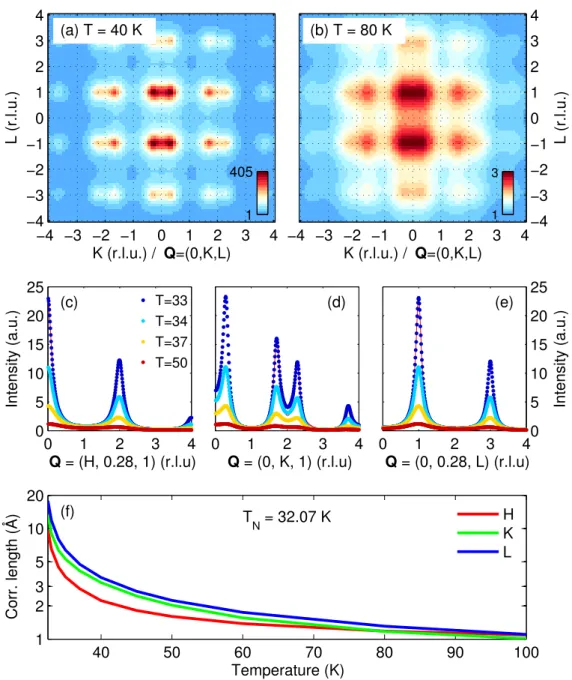
![Figure 4.16.: Calculated neutron intensity for TbMnO 3 along (a) [H, 0.28, 1], (b) [0, K, 1] and (c) [0, 0.28, L] using model M-II](https://thumb-eu.123doks.com/thumbv2/1library_info/3698877.1505930/64.892.166.730.167.378/figure-calculated-neutron-intensity-tbmno-using-model-ii.webp)