Neutron Scattering Studies on Magnetic Excitations in Complex Ordered Manganites

(1)

Neutron Scattering Studies on Magnetic Excitations in Complex Ordered Manganites

Daniel Sen

(2)

on Magnetic Excitations in Complex Ordered Manganites

Inaugural Dissertation

zur

Erlangung des Doktorgrades

der Mathematisch-Naturwissenschaftlichen Fakultät der Universität zu Köln

vorgelegt von

Daniel Sen

aus Köln

Köln, September 2007

(3)

Berichterstatter: Prof. Dr. M. Braden Prof. Dr. M. Vojta Prof. Dr. B. Büchner Vorsitzender

der Prüfungskommission: Prof. Dr. L. Bohatý

Tag der letzten mündlichen Prüfung: 29. Oktober 2007

(4)

Heinrich Böll

(5)

1 Introduction

An entity might be considered as complex if it is consisting of many dierent and connected parts [1]. In light of this denition, transition-metal oxides are of spe- cial complexity, as their physical behavior arises from the sophisticated interplay between many dierent degrees of freedom including spin, charge, orbital, and the crystal lattice [2]. The electronic correlations often result in a competition or even coexistence of states with very dierent characteristics, and small external pertur- bations can lead to a giant response and novel behavior, as e. g. high-temperature superconductivity in cuprates [3] and the colossal change of the electric resistivity in a magnetic eld in perovskite manganites, known as CMR-eect [4].

In manganites, a slight change of parameters tunes between ground states with contrasting properties, and the competition between various interactions results in a very rich one might as well call it complex phase diagram containing a variety of phases. In the neighborhood of two distinct states, the balance between the dierent degrees of freedom is often very subtle and can easily be manipulated.

The most popular consequence is the CMR-eect, which today is considered as the switching between a ferromagnetic metallic and an antiferromagnetic charge- ordered state [4, 5]. A second remarkable feature, appearing at the border of two dierent antiferromagnetic states, is a gigantic magnetoelectric coupling, which has recently been discovered in multiferroic manganites [6] and which, due to its possible technical applications, immediately attracted a lot of interest.

The present thesis analyzes the magnetic excitation spectrum of three dierent manganese oxides related to these eects, undoped LaSrMnO 4 , charge-ordered La 1 / 2 Sr 3 / 2 MnO ₄ and multiferroic TbMnO ₃ , which were studied by means of in- elastic neutron scattering. Common to all three systems is a complex magnetic ordering, and the magnetic state is strongly inuenced by the interplay with other degrees of freedom. Conversely, understanding the static and dynamic magnetic properties does not yield insight only into the magnetic, but also e. g. into the orbital correlations.

LaSrMnO 4 is the two-dimensional analog of the parent compound of manganese

oxides, LaMnO ₃ . Although considered as a simple antiferromagnet in the recent

literature [7], the spin-wave spectrum is not consistent with this simple approach,

and the present results provide signicant evidence for a heterogenous magnetic

ground state driven by a close correlation of magnetic and orbital degrees of free-

dom. Structurally similar to LaSrMnO 4 , the hole-doped system La 1 / 2 Sr 3 / 2 MnO ₄ ex-

(8)

hibits the typical cooperative ordering of charges, orbitals, and spins, generic for manganites with a rational fraction of charge carriers. Although the ordered state has attracted a lot of interest since its prediction half a century ago [8], and de- spite the great importance for the understanding of the CMR-eect, even the ground-state properties of the ordered state are not well established and dierent concepts are still controversially discussed [9]. Analyzing the spin-wave dispersion allows to distinguish between the dierent proposals, unambiguously conrms the predictions of the classical model, and reveals certain similarities between the anti- ferromagnetic charge-ordered and the ferromagnetic state, which seem to compete in a wide parameter range resulting in the famous metal-insulator transition in perovskite manganites.

The orthorhombic manganite TbMnO ₃ is one of the pivoting materials in the fas- cinating class of multiferroic oxides [10]. The dynamics of systems with simultane- ous magnetic and ferroelectric order is predicted to be controlled by new collective excitations regarded as hybridized magnon-phonon vibrations [11], and the strong magnetoelectric coupling in TbMnO ₃ allows, for the rst time, the experimental observation of such excitations. The physical properties of TbMnO ₃ are well un- derstood by the momentum, temperature, and eld dependence of the hybridized uctuations, and the experimental results are in excellent agreement with recent theories connecting the observed ferroelectricity with complex magnetic ground states [12, 13].

The present thesis is divided into six chapters, which are arranged according

to ascending physical complexity. These introductory remarks are followed by

a brief introduction into the technique of inelastic neutron scattering in chapter

2. Subsequently, chapter 3, the rst of three experimental chapters, discusses

the magnetic and orbital correlations of the single-layered manganite LaSrMnO 4 .

Chapter 4 is the longest section of this thesis and is dedicated to the charge- and

orbital-ordered state in half-doped La 1 / 2 Sr 3 / 2 MnO ₄ , including the analysis of the

excitation spectrum in La 1 / 2 Sr 3 / 2 MnO ₄ , as well as the thermal evolution and the

doping dependence of the ordered state. The last experimental chapter 5 deals

with the characterization of the excitation spectrum of multiferroic TbMnO ₃ , and

the thesis is nally closed by a summary of the most relevant results in chapter 6.

(9)

2 Magnetic neutron scattering

Only four years after the discovery of the neutron by J. Chadwick in 1932 it has been demonstrated that neutrons can be diracted by condensed matter. More- over, due to its magnetic moment neutrons are not only diracted by crystalline, but also by magnetic lattices, as rst has been suggested by Bloch in 1936 and fteen years later has been veried in the pioneering work of Shull, Wollan and Strauser [14, 15]. Since then, and especially with today's advanced reactor sites and modern spallation sources neutron scattering has become one of the most powerful and versatile experimental techniques for probing condensed matter.

The fundamental physical properties of the neutron provide insight into the static and dynamical correlations of modern materials, which mostly are hardly accessible with alternative techniques. In elastic neutron studies one takes advan- tage of the short-range nature of the nuclear interaction potential, which yields a high visibility of light elements and a sizable contrast even between dierent iso- topes, and of the neutron's magnetic moment, which interacts with the magneti- zation density of unpaired electrons and oers a unique method to study magnetic correlations on a microscopic scale. In the eld of dynamic correlations neutron scattering is today by far the most important experimental tool, since only neu- trons allow a sizeable momentum transfer at energy scales valid for collective exci- tations like phonons and magnons. Due to its rest mass m n = 1.674928 × 10 ⁻²⁴ g a thermal neutron with wavelength λ =2.4 Å possesses an energy E ≈ 14 meV , which is of the order of typical collective excitations. In contrast, the energy of a photon with similar wavelength is 7 − 8 orders of magnitude larger and an excel- lent energy resolution and thus a huge experimental eort is required to resolve a meV-change in the photon energy, which is available only since a few years at the most brilliant x-ray sources. Indeed, the recent developments in the wide eld of spin and lattice dynamics are founded on experimental results achieved with inelastic neutron scattering.

2.1 Neutron scattering formulas

In a neutron scattering experiment the count rate C of neutrons with energy E in

the interval E ⁰ and E ⁰ + d E ⁰ scattered into a given solid angle d Ω normalized to

the incident neutron ux I ₀ is given by the dierential cross section _d _Ω ^d ² _d ^σ _E 0 . In this

section we recall briey the basic expressions for the cross section of elastic and

(10)

inelastic scattering and connect the cross sections with the physical properties of the system under investigation. For an extended derivation and a detailed discussion of the various cross sections we refer, however, to the classical review articles and textbooks on neutron scattering [1620].

Let k _i be the wave vector and σ _i the spin state of the incident neutron. If we label the initial and nal states of the scattering system by quantum numbers λ _i and λ _f the dierential cross section for a scattered neutron with nal wave vector k _f and nal spin state σ _f is given by Fermis Golden Rule:

d ² σ d Ω d E ⁰

k i →k _f

= 1 N

k f

k _i m

2π ~ 2 X

λ i σ i

p _λ _i p _σ _i X

λ f σ f

|hk _f σ _f λ _f |V |k _i σ _i λ _i i| ² δ( ~ ω + E _λ _i − E _λ _f ) (2.1) with the energy of the incident and scattered neutrons E _i and E _f , the energy change of the scattering system ~ ω , the probability p _j to nd the system or the neutron in the state j and the interaction potential V . This masterformula of neutron scattering is a very general result as no assumption about the interaction potential V (r) is made, and the determination of the cross sections for the various magnetic and nuclear scattering processes has reduced to the elaboration of the matrix elements of the interaction potential V (r) .

The interaction of neutrons with matter can be divided into two parts a nuclear part due to the scattering of the neutron at the nucleus and a magnetic part due to the magnetic dipole interaction between the magnetic moment of the neutron and the electrons of an atom. Since the focus of this thesis is on magnetic correlations, we will state the scattering formulas for the nuclear interaction briey and discuss afterwards the magnetic interaction in some more detail.

2.1.1 Nuclear neutron scattering

The nuclear forces which cause the nuclear scattering act on a scale much smaller than the typical wavelength of a neutron. The scattering potential of an assembly of N atoms at positions R j of, for simplicity, a single element can therefore be modeled as

V _N (r) = 2π ~ ² m

X

j

bδ(r − R _j ) (2.2)

with a single parameter b describing the scattering power of the atom j . The

scattering length b is not only element specic, but does also depend on the vari-

ation of isotopes and on the total spin of the nucleus-neutron system. Dening

the scattering vector Q = k _f − k _i the dierential cross section for coherent and

(11)

2.1 Neutron scattering formulas

incoherent nuclear scattering reads as:

d ² σ d Ω d E ⁰

coh

= 1 N

σ _coh 4π

1 2π ~

k _f k _i

X

jj ⁰

∞

Z

−∞

h e ^−iQR ^j ⁽⁰⁾ e ^QR ^j ⁰ ^(t) i e ^iωt d t (2.3)

d ² σ d Ω d E ⁰

inc

= 1 N

σ _inc 4π

1 2π ~

k f

k _i X

j

∞

Z

−∞

h e ^−iQR ^j ⁽⁰⁾ e ^QR ^j ^(t) i e ^−iωt d t (2.4) where σ _coh = 4πb ² and σ _inc = 4π(b ² − b ² ) . We will focus only on the coherent part in the following, as the incoherent part does not give interference eects between dierent atoms j and j ⁰ .

It is useful and common practice to express the cross section eq. 2.3 in terms of correlation functions: If we dene the coherent scattering function S(Q, ω) as

S(Q, ω) = 1 N

1 2π ~

∞

Z

−∞

X

jj ⁰

h e ^−iQR ^j ⁽⁰⁾ e ^QR ^j ⁰ ^(t) i e ^−iωt d t (2.5)

the cross section for coherent scattering reduces to d ² σ

d Ω d E ⁰

coh

= σ _coh 4π

k _f

k _i S(Q, ω). (2.6)

The scattering function S(Q, ω) describes the correlations in space and time be- tween an atom j at time t = 0 at site R _j and a second atom j ⁰ at a nite time t at site R _j ⁰ . Obviously, the scattering function contains all desired informations about the static and dynamic behavior of the system under investigation.

Elastic nuclear Bragg scattering Consider a crystal with translation invariance j and d atoms in the unit cell. Because of thermal motion each atom will oscillate around its equilibrium position d and the position of atom d is

R _jd = j + d + u _d (j, t), (2.7) where u d (j, t) is the displacement from the equilibrium. The translation invariance of the crystal reduces the double sum in eq. 2.5 to a single summation over the distances j − j ⁰ and for elastic scattering ( ω = 0 ) the dierential cross section transforms to

d σ d Ω

el coh

= (2π) ³ v 0

X

τ

|F _N (Q)| ² × δ(Q − τ ) (2.8)

(12)

with a reciprocal lattice vector τ , the unit cell volume v ₀ and the nuclear structure factor F _N (Q) dened by

F _N (Q) = X

d

b _d e ^iQd e ^−W ^d ^(Q) . (2.9) The Debye-Waller factor exp(−W _d (Q)) = exp(−h(Qu(j, d)) ² i) takes into account the mean square displacement of each atom and decreases the observed intensity of a Bragg peak with increasing |Q| .

One phonon cross section The coherent one phonon cross section is derived from the expansion of the displacement correlation functions hQu _d (j, 0)Qu _d (j ⁰ , t)i and can shown to be:

d ² σ d Ω d E ⁰

inel coh

= k _f k i

(2π) ³ 2v 0

X

τ

X

ν,q

1 ω ν (q)

X

d

b _d e ^−W ^d ^(Q) e ^iQd · Qe _d (q, ν)

√ M d

2 ×

[n _ν (q) δ(E _i − E _f + ~ ω _ν (q))δ(Q + q − τ )]

+ [(n _ν (q) + 1) δ(E _i − E _f − ~ ω _ν (q)δ(Q − q − τ )]

(2.10)

with the mass M _d of atom d , the thermal population factor for Bose particles n ν (q) and the polarization vector e d (q, ν) and the frequency ω ν (q) of the phonon ν [17]. The coherent one phonon cross section can be divided into two parts: The δ -functions in eq. 2.10 give the conservation of both energy and momentum in the scattering process and it is easily seen that the second line in eq. 2.10 describes the annihilation of a phonon and thus an increase of the neutron's energy in the scattering process, while the third line denes the creation of a phonon and an energy loss of the neutron. The contribution of these two processes to the cross section is asymmetric with respect to the principle of detailed balance: The annihilation of a phonon with frequency ω is counted with the single population function n _ν (q) , while the creation of a phonon contributes with a prefactor n _ν (q)+

1 to the summation.

2.1.2 Magnetic neutron scattering

In the case of magnetic neutron scattering the interaction potential between a neutron in spin state σ and a moving electron of momentum p and spin s is

V _M (r) = −γµ _N 2µ _B σ ·

"

curl s × R ˆ R ²

! + 1

~

p × R ˆ R ²

#

(2.11)

where γ = 1.9132 is the gyromagnetic ratio, µ _n and µ _B are the nuclear and

the Bohr magneton and R is the distance vector between the electron and the

(13)

2.1 Neutron scattering formulas neutron. Restricting ourselves for the moment to an unpolarized beam of neutrons, inserting the potential V _M into the masterformula eq. 2.1 results after some more sophisticated algebra in the dierential cross section for pure magnetic scattering

d ² σ d Ω d E ⁰

mag

= (γr ₀ ) ²

~ k _f k _i

X

α,β

δ α,β − Q _α Q _β Q ²

S ^αβ (Q, ω) (2.12) with the classic radius of the electron r ₀ and the summation over the spatial coordinates α, β ∈ [x, y, z] . The magnetic scattering function S (Q, ω) is dened by the spin-spin correlations

S ^αβ (Q, ω) = 1 2π

∞

Z

−∞

X

j,d 1

2 g _d f _d (Q) e ^−W ^d ^(q) e ^iQ(j+d) hS ₀ ^α (0)S _j+d ^β (t)i e ^−iωt d t (2.13) where g is the Landé factor, S describes the local magnetic moment and f d (Q) the atomic form factor of atom d in unit cell j .

The magnetic interaction leads in addition to magneto-vibrational scattering which is not included in the above cross section [17].

Elastic magnetic scattering For elastic magnetic scattering we have to eval- uate the scattering function S(Q, ω = 0) . Dening in analogy with the elastic structural scattering the magnetic structure factor

F _M (Q) = γr ₀ X

d 1

2 g _d f _d (Q)hS _d i e ^iQd e ^−W ^d ^(Q) (2.14) and F _M⊥ = ˆ Q × F _M × Q ˆ with Q ˆ = Q/Q , the cross section for elastic magnetic scattering reads

d σ d Ω

el mag

= 2π ³ v ₀

X

τ M

|F M,⊥ (τ _M )| ² × δ(Q − τ _M ), (2.15) and the form of the elastic magnetic cross section looks very similar to the one for nuclear scattering. However, there are some very crucial dierences which turn out to be fruitful and will later on allow us to easily separate magnetic from nuclear scattering: In the magnetic structure factor the scattering power of each spin is determined by the prefactor p = ¹ ₂ γr 0 gf d (Q) , ¹ which due to the atomic form factor f _d (Q) rapidly decreases with increasing |Q| and thus exhibits a contrary |Q| -dependence as in the nuclear case, where the scattering length b is

1 Notice that p has the dimension of a length; for Q = 0 the magnetic scattering length p ₀ =

1 2 γr ₀ = 0.2695 ×10 ⁻¹² cm is of the same order as a typical nuclear scattering length b .

(14)

0.1 0.2 0.3 0.4 0.5 0.6 0.7 0.8 0.9

80 60 40 20 0

8 6 4 2 0

(deg.)

|Q|(Å

-1 )

Figure 2.1: |Q| -dependence of mag- netic scattering Simulation of the |Q| - dependence of the eective magnetic scattering length f _Mn ³⁺ (Q) sin(α) of a Mn ³⁺ -ion for various angles α between the scattering vector Q and the magnetic moment S [21].

Q -independent. This behavior is superimposed by the general scattering law for magnetic scattering, that only the magnetization perpendicular to the scattering vector Q contributes to the cross section.

To resume, magnetic scattering always exposes a characteristic decrease with

|Q| , which furthermore depends sensitively on the angle α between the scattering vector Q and the magnetic moment S , see Fig. 2.1.

Inelastic scattering by spin waves If we choose the quantization axis to be along z and if we assume the total z-component of the magnetization S ^z to be a constant of motion (as is e. g. the case for the Heisenberg Model) only the terms α = β contribute in eq. 2.13 to the scattering function S(Q, ω) and we obtain for a Bravais lattice:

d ² σ d Ω d E ⁰

mag

∝

1 − Q ² _z Q ²

1 2π ~

Z ∞

−∞

X

j

e ^iQj hS ₀ ^z (0)S _j ^z (t)i e ^−iωt d t

+ X

α∈[x,y]

1 − Q ² _α Q ²

1 2π ~

Z ∞

−∞

X

j

e ^iQj hS ₀ ^α (0)S _j ^α (t)i e ^−iωt d t.

(2.16)

In linear approximation the rst part of eq. 2.16 is time independent and re- produces the elastic magnetic scattering we have just discussed, and the inelas- tic scattering by spin waves is determined only by the transverse correlations hS ₀ ^x,y (0)S _j ^x,y (t)i .

However, evaluating the transverse spin correlation terms for a given complex

magnetic structure is in general a non-trivial task. To derive a semi-classical

picture of the magnetic excitations in an ordered structure, which later on will be

helpful in the interpretation of the observed spectra, we discus here the simplest

possible case the Heisenberg FM with nearest-neighbor exchange only. The

(15)

2.1 Neutron scattering formulas

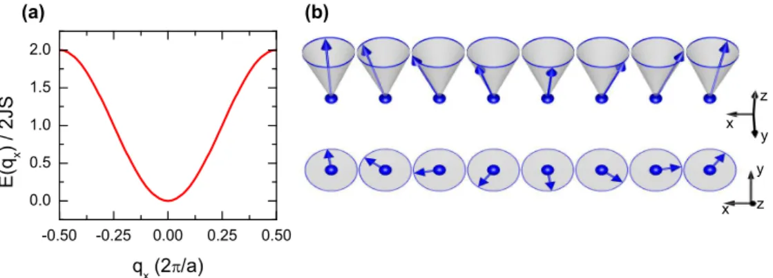
-0.50 -0.25 0.00 0.25 0.50 0.0

0.5 1.0 1.5 2.0

z y

x y x (b)

E(q x

)/2JS

q x

(2 /a) (a)

z

Figure 2.2: Spin waves in the FM Heisenberg model Magnon dispersion for the FM Heisenberg model calculated from eq. 2.18 (a), and snap shot of a spin wave as a precession of the transversal moment in the limit of large S (b)

Hamiltonian of a Heisenberg ferromagnet on a square lattice H = − X

i,j

J _i,j S _i S _j = − X

i,j

J _i,j

S _i ^z S _j ^z + ¹ ₂

S _i ^† S _j ⁻ + S _i ⁻ S _j ^†

(2.17) is easily diagonalized using the Holstein-Primako transformation yielding the spin-wave dispersion, see Fig. 2.2:

~ ω(q) = 4S(J _q=0 − J(q)) = 4J S · (2 − cos(q _x a) − cos(q _y a)). (2.18) The transverse cross section for the Heisenberg FM is nally given by

d ² σ d Ω d E ⁰

inel mag

= (γr ₀ ) ^{2 1} ₂ S( ¹ ₂ gf (Q)) ² k _f k _i

1 + Q ² _z Q ²

e ^−W ^(Q)

× X

τ M ,q

n(q)δ(E i − E f + ~ ω q )δ(Q − q − τ M )

+ (n(q) + 1)δ(E _i − E _f − ~ ω _q )δ(Q + q − τ _M ) ,

(2.19)

and consists as for phonon scattering of two parts describing separately the an- nihilation and creation of a magnon with energy ~ ω q by the neutron [17]. In the limit of large moments S _i the expectation values of the transverse correlations obey the equations

hS ₀ ^x (0)S _j ^x (t)i ∝ cos(qj − ωt) and (2.20a)

hS ₀ ^y (0)S _j ^y (t)i ∝ sin(qj − ωt), (2.20b)

and a spin wave can be visualized as a precession of the spins around the z -axis,

see Fig. 2.2.

(16)

Polarization analysis So far we have always integrated out the spin states of the neutron and the cross sections for nuclear and magnetic scattering did not depend explicitly on the neutron spin σ . However, with today's advanced spectrometers and polarization devices it is possible to manipulate very accurately the spin σ of the neutron and the technique of polarized neutron scattering yields additional, often very important details about the system under investigation.

A general treatment of the polarization analysis is quite complex [20]; here, we will restrict ourselves to the case of the longitudinal polarization analysis intro- duced rst by Moon, Riste and Koehler [22], and analyze only the projection of the nal polarization P _f of the scattered neutrons on the direction of the initial polarization P _i .

For the moment, we dene a coordinate system (ζ, ς, ξ) for the spin space and take the spin-quantization axis to be along ξ . Treating the spin state of the neutron separately, each cross section using unpolarized neutrons will now give rise to two cross sections in which the spin state of the neutron changes from the

|±i to the |∓i state in the scattering process (spin-ip scattering), and two cross sections in which the spin state remains unchanged (non spin-ip scattering).

Ignoring the incoherent scattering from the magnetic moments of the nuclei these cross sections are determined by the four transition amplitudes:

d ² σ d Ω d E ⁰

|±i→|±i

∝

N (Q) ± M _⊥ ^ξ (Q)

2 and (2.21a)

d ² σ d Ω d E ⁰

|±i→|∓i

∝

M _⊥ ^ς (Q) ± iM _⊥ ^ζ (Q)

2 (2.21b)

with the Fourier transform of the nuclear and magnetic density N (Q) and M (Q) [22]. As aforementioned, in the magnetic channel only the component M ⊥ (Q) of the magnetic density M (Q) perpendicular to the scattering vector Q contributes to the cross section.

It is now intriguing to discuss the implications derived directly from eq. 2.21, rather than reciting the bulky expressions for the various cross sections. ² In- specting the cross sections eq. 2.21 the fundamental rules for the longitudinal polarization analysis are immediately derived:

(i) Nuclear scattering does not ip the spin of the neutron.

(ii) The components of M ⊥ (Q) parallel to P _i always contribute to the non spin- ip scattering.

(iii) The magnetic components perpendicular to both P i and Q are always de- tected in the spin-ip channel.

2 A comprehensive discussion of this lengthy algebra is e. g. given in the classical textbook on

neutron scattering by Marshall and Lovesey [17] and in the more modern review by Chatterij

[20].

(17)

2.1 Neutron scattering formulas

NSF SF

P _i k x ˆ (M _⊥ ^y ) ² + (M _⊥ ^z ) ² P _i kˆ y (M _⊥ ^y ) ² (M _⊥ ^z ) ² P _i kˆ z (M _⊥ ^z ) ² (M _⊥ ^y ) ²

Table 2.1: Contribution of the in-plane and out-of-plane eective magnetic moments M _⊥ ^y and M _⊥ ^z to the non spin-ip (NSF) and spin-ip (SF) channels for various choices of the incident polarization: parallel to the scattering vector Q ( x ), perpendicular to Q within (y), and perpendicular to both Q and the scattering plane (z). For convenience, we neglect the inuence of chiral terms and scattering due to nuclear-magnetic interfer- ence, which would give additional contributions in the SF- P _x - and NSF- P _y,z -channels, see e. g. Ref. [20].

These simple rules exhibit their full beauty upon combining the cross sections for dierent choices of the incident polarization P _i : We dene the spatial coordinates (x, y, z) by xkQ ˆ , y⊥Q ˆ within and z ˆ ⊥ Q perpendicular to the scattering plane, as will always be the case for the polarized neutron data presented in this thesis.

Now, if P _i kˆ x , magnetic intensity is only observed in the SF-channel, while for P _i kˆ y only the vertical component M _⊥ ^z (Q) of the magnetization density contributes to the SF-scattering, see Tab. 2.1.2. Taking the dierence between the two observed intensities the common background cancels out and we obtain directly the in-plane component of the eective moment M _⊥ ^y (Q) :

d ² σ d Ω d E ⁰

^|±i→|∓i

P kˆ x

−

d ² σ d Ω d E ⁰

^|±i→|∓i

P k y ˆ

∝ |M _⊥ ^y (Q)| ² . (2.22) Measuring the various SF cross sections, respectively their dierences provides thus the opportunity to dene all three components of the magnetic density inde- pendently.

In conclusion, the longitudinal polarization analysis enables to recover the spa- tial details of the magnetic density distribution of a magnetically ordered struc- ture, like e. g. in diraction experiments the direction of the ordered moment, or, in the case of inelastic scattering, the eigenvectors of magnetic excitations in addition to their eigenfrequencies ω _q [17, 22].

Crystal-eld excitations So far, we have discussed the scattering of collective phenomena like e. g. spin waves. However, neutron scattering is also sensible to local excitations, which will concern us especially in the discussion of the excitation spectrum of the multiferroic compound TbMnO ₃ .

In a crystal, the surrounding electrostatic eld as well as the spin-orbit coupling

lifts the degeneracy of an unlled 4f ⁿ conguration of a rare-earth ion and gives

(18)

rise to J -multiplets. The neutron can excite the rare-earth ion from a lower to a higher state with a corresponding loss of the neutron energy or deexcite from a higher to a lower energy level. The obtained spectrum reects the splitting of the J -multiplet and superimposes the scattering by collective excitations: If the dierent crystal-eld states have eigenfunctions |ii with energies δ _i and thermal population n i , the cross sections for a crystal-eld excitation is determined by a series of delta functions:

d ² σ d Ω d E ⁰

CEF

∝ k _f

k _i f(Q) ² X

i,j

n i |hi|J ⊥ |ji| ² δ(δ i − δ j − ~ ω), (2.23) and again only the component J ⊥ of the momentum J perpendicular to Q con- tributes to the cross section [23]. The best way to separate the dierent con- tributions is to study the Q -dependence, since local excitations do not posses a characteristic dispersion.

2.2 The triple-axis spectrometer

The experimental realization for using neutrons as a spectroscopic tool for de- termining the dispersion of phononic and magnetic excitations is the triple-axis spectrometer (TAS) installed at a reactor neutron source. First build by Brock- house in the late 1950s, a TAS spectrometer allows the full control over the entire (Q, ω) -space within the borders set by the scattering kinematics in a wide en- ergy and momentum transfer regime. In addition, today's spectrometers are very exibel and extreme sample environments as e. g. strong magnetic elds and ad- vanced neutron techniques like polarization analysis can often be mounted onto these machines.

The TAS spectrometers used for the studies in this work are situated at the four major reactor sources in Germany and France the Hahn-Meitner Institut (HMI) in Berlin, the Forschungsneutronenquelle Heinz Maier-Leibnitz (FRM II) in Munich, the Laboratoire Léon Brillouin (LLB) near Paris and the Institut Laue Langevin (ILL) in Grenoble. According to the energy spectrum of the incident neutrons from the reactor the various spectrometers are divided into three categories: cold, thermal and hot. At the cold spectrometers, like FLEX at the HMI, PANDA at the FRM II, 4F at the LLB and IN12 and IN14 at the ILL, the incoming neutrons are moderated inside the reactor to energies of

∼ 25 K . These machines are well suited for high-resolution studies at low energies

~ ω between 0 − 10 meV . Thermal spectrometers with incident energies around

300 K are dedicated to the energy regime ~ ω = 10 − 100 meV and are optimized to

a high neutron ux at the sample with reduced energy and Q resolution. Thermal

spectrometers used in this thesis are the PUMA spectrometer installed at the FRM

II, the 1T at the LLB and the IN22 at the ILL. Even higher energy transfers up

(19)

2.2 The triple-axis spectrometer

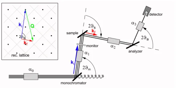
Figure 2.3: General layout of a TAS-spectrometer Classical W-conguration of a triple-axis spectrometer with the three movable axis, the horizontal collimation α _i and the trajectory of the neutron in real and reciprocal space.

to 500 meV can be achieved at hot sources, which are, however, not used in this work.

2.2.1 Basic principles of a TAS spectrometer

Although the characteristics of the various spectrometers are quite dierent, their general layout is very similar, see Fig. 2.3 and 2.4. In order to access a general point in the four-dimensional (Q, ω) -space it is sucient to control both the direction and the modulus of the wavevector of the neutron k _i before and k _f after the scattering process. The momentum transfer is then given by Q = k _f − k _i and the energy transfer by ~ ω = _2m ^~ ²

n (k _i ² − k ² _f ) . In a triple-axis spectrometer k _i and k _f are usually manipulated by applying Bragg's law for reection from a crystal. From the incident beam of neutrons with a continuous energy spectrum determined by the temperature of the moderator a specic energy k _i ² is selected by elastic Bragg reection from a monochromator crystal xing k _i in the reactor frame:

k _i = 2π 2d M sin 2ϑ M

, (2.24)

with the distance d _M between a set of crystal planes and the associated grazing

angle ϑ _M . After the scattering at the sample the beam of neutrons is again poly-

chromatic due to inelastic processes and a dened energy k _f ² in a given direction

k _f can be selected by a second Bragg reection from an analyzing single crystal

before the neutrons are counted in the detector unit. The spatial arrangement of

(20)

Figure 2.4: Cold triple-axis spectrometer 4F at the LLB The primary spec- trometer with the monochromator unit is marked by green, the sample area equipped with a closed-cycle cryostat and the typical Helmholtz coils for longitudinal polarization analysis by blue, and the secondary spectrometer with the monochromator crystal by red annotations. The reactor core is situated in the left and the neutron's trajectory from left to right is marked in yellow.

the monochromator, the sample, the analyzer and the detector thereby denes a plane in the coordinate system of the reactor to which the possible choices for the set (k _i , k _f ) is restricted. The momentum transfer Q is thus obviously limited to a single particular crystallographic plane, which has to be chosen properly at the beginning of each experiment!

Besides the reactor, the most important components which determine the per-

formance of a spectrometer are the monochromator and the analyzer. Typically,

for unpolarized studies the neutrons are analyzed using the (0 0 2) -reection of

pyrolytic Graphite (PG), and in the case of polarized experiments by the (1 1 1) -

reection of a Heusler alloy . At lower incident energies E _i . 40 meV the PG (0 0 2)

reection is also commonly used for monochromation, while the thermal spectrom-

eters provide additionally a Cu (1 1 1) or Cu (2 2 0) monochromator for higher neu-

tron energies. To increase the neutron intensity, the monochromator as well as the

analyzer consists of several blades which can be curved vertically (and sometimes

also horizontally) to focus the divergent neutron beam to the sample position.

(21)

2.2 The triple-axis spectrometer

0 25 50 75 100 125

1.0 1.5 2.0 2.5 3.0 3.5 4.0 4.5

(b)

neutronintensity (arb.units)

vertical curvature (arb. units) (a)

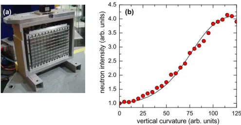
Figure 2.5: Double-focusing PG monochromator at the PANDA spectrom- eter Double-focusing PG(0 0 2) monochromator of the PANDA spectrometer consisting of 117 single blades mounted on the curvature mechanics (a). Measured elastic intensity from a Vanadium standard as a function of the vertical monochromator curvature with a neutron energy of k f =1.55 Å ⁻¹ (b).

With this type of curvature on both the monochromator and the analyzer side the measured intensity can easily gain more than a factor 10 , see Fig. 2.5, which more than overcompensates the small decrease in resolution due to the focusing. All of the inelastic experiments presented in this thesis have been performed using fully focusing congurations.

The transfer of energy in the scattering process can be realized in two alternative ways one may either x the energy of the incident or of the nal neutrons to a constant value and vary the other. If possible, we always choose the second alter- native with k _f xed, since in this conguration the spatial angles on the secondary spectrometer are held constant and the angular dependence of the reectivity of the analyzer has not to be taken into account. Checking the ux of the neutrons behind the monochromator allows to easily correct for changes in the reectivity of the monochromator and the intensity spectrum of the reactor source simply by normalization to the monitor countrate.

The actual value of the xed nal neutron energy depends decisively on the

velocity spectrum of the incident neutron beam. The Maxwell distribution for

thermal neutrons has a broad maximum centered at ≈ 50 meV , while on a cold

spectrometer the incident ux is maximized around ≈ 5 meV . Therefore, thermal

spectrometers perform best with k _f = 3 − 4 Å ⁻¹ , as on a cold machine the incident

ux limits the nal energy to k _f < 2 Å ⁻¹ . As the density of the reciprocal space

increases with decreasing wavelengths, the resolution in both Q and ω is best

on a cold source with small xed nal energies the typical energy resolution

determined by the width of the incoherent line of a Vanadium standard on a cold

(22)

TAS with k _f xed to 1.5 Å ⁻¹ of ∆E ≈ 50 µ eV is an order of magnitude better than on a thermal spectrometer with ∆E ≈ 800 µ eV for k _f =2.662 Å ⁻¹ .

A major problem on a triple-axis spectrometer are higher-harmonic wavelengths, which also satisfy the Bragg condition at the monochromator and analyzer. To reduce the contamination by these parasitic wavelengths appropriate lter based once more on Bragg reection are commonly used: The maximum wavelength for which Bragg scattering can occur is λ _max = 2d _max with a maximum d -spacing d _max . For wavelengths greater than λ _max the lter is transparent, and choosing a mate- rial with an appropriate d _max allows to diminish contaminations by higher-order neutrons. In the low-energy regime we have always used polycrystalline Beryllium with an upper cut-o energy of 5.2 meV (≈ 1.58 Å ⁻¹ ) as a band-pass lter. In the higher-energy regime at thermal spectrometers lters of pyrolytic Graphite are the best choice. However, PG-lters are restricted to certain energies with a high transmittance for λ and simultaneously low transmittance, of the order of 10 ⁻⁴ , for λ/2 . These energies are well known to be at 13.70 meV, 14.68 meV, 30.6 meV and 34.8 meV, energies which appear in almost all publications on inelastic neutron scattering.

2.2.2 The resolution function

One of the most important aspects in the planning, realization and analysis of a TAS experiment concerns the resolution of the chosen instrument. As the proper manipulation of the resolution is of such immense importance in a TAS mea- surement, we will present the basic properties of the resolution function in the following paragraph. For further insights into this widespread problematic we, however, refer to the original literature [2426] and to the excellent illustration in the practical textbook of the Brookhaven group [19].

In a TAS experiment a selected point (Q ₀ , ω ₀ ) of the four-dimensional (Q, ω) - space is selected by the proper settings of the scattering angles at all three axis of the spectrometer, see Fig. 2.3. However, the nite collimation and the imper- fect mosaicity of the monochromator crystals allows neutrons corresponding to the scattering event (Q ₀ + ∆Q, ω + ∆ω) to reach the detector as well, and the resolution function R of a TAS instrument is dened as the probability of detec- tion of neutrons as a function of ∆Q and ∆ω when the instrument has been set to measure a scattering process corresponding to the point (Q ₀ , ω ₀ ) [24]. Quite obviously, for any given scattering function S(Q, ω) the observed intensity in an experiment is determined by the convolution of the scattering function with the instrument's resolution function R ,

I (Q 0 , ω 0 ) = Z

R(Q − Q 0 , ω − ω 0 )S(Q, ω) dQ dω. (2.25)

It is very useful to visualize the resolution function as a four-dimensional ellip-

(23)

2.2 The triple-axis spectrometer soid in (Q, ω) space. The ellipsoid is centered at (Q ₀ , ω ₀ ) and the points at the borders of the ellipsoid possess a probability of 50 % to reach the detector unit, see Fig. 2.6. The exact size and the spatial orientation of the ellipsoid depends, of course, sensitively on the neutron wavelength, the type of the monochromator crystals, or more precisely on the selected d-spacing, on the scattering sense at the three axis, and on the selected collimation restricting the divergence of the beam.

The control of the spatial orientation of the resolution ellipsoid is often of great importance in an experiment, especially when dealing with dispersive excitations.

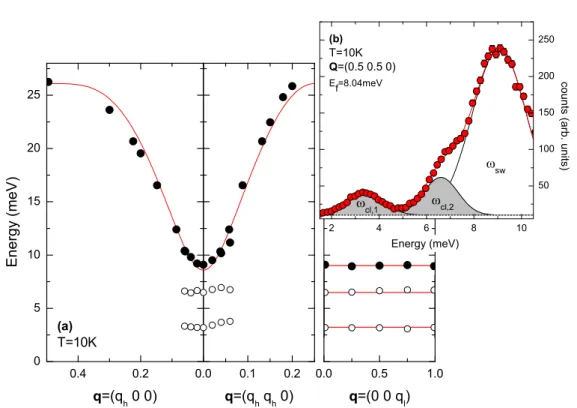
In Fig. 2.6a we show the low-energy part of the spin-wave dispersion of the charge and orbitally ordered compound La 1 / 2 Sr 3 / 2 MnO ₄ , which is analyzed in detail in chap. 4. Leaving a detailed discussion to one of the following chapters, for the moment the dispersion can well be understood by two equivalent magnon branches propagation outward from the magnetic zone center Q = (0.75 0.75 0) , correspond- ing to the modes traveling in the ±[q _h −q _h 0] directions. Typically, such a dispersion is mapped experimentally by scanning the momentum transfer Q at a constant energy E , as is indicated by the dotted red line in Fig. 2.6a. However, the exper- imental response depends decisively on the relative orientation of the resolution ellipsoid and the dispersion surface in the four-dimensional (Q, ω) -space, and the experimentally observed signal for both (equivalent) branches will be dierent:

For one of the two sides the slope of the dispersion is inclined to the long axes of the ellipsoid, and at this focusing side the convolution of the resolution function with the dispersion surface yields a sharp signal. On the other side, the long axes of the ellipsoid are, in the most extreme case, oriented perpendicular to the dis- persion surface resulting in a very broad response, see Fig. 2.6b. Of course, in an experiment it is always preferable to choose an appropriate Q -position allowing to work on the focusing side!

So far, the argumentation seems reversed, as usually the dispersion surface is not known before the experiment. Inverting however the above argumentation, the scattering function S(Q, ω) has to be extracted by a deconvolution of the observed intensity and the experimental resolution. The resolution matrix of a TAS instrument can easily be calculated [24], we usually use the ResLib code implemented for Matlab [27]. An arbitrary scattering function S(Q, ω) can then be convoluted with the resolution ellipsoid and subsequently be tted to a set of data to extract the desired parameters, as e. g. the dispersion relation ~ ω(q) of a magnon excitation. A typical example is shown in Fig. 2.6b, where the exper- imental data are tted to a model dispersion convoluted with the experimental resolution. Note, that in addition to the physical parameters describing the prop- erties of the scattering function S(Q, ω) there is only one adjustable parameter for all data points scaling the neutron intensity in this procedure.

In principle, iterating the above algorithm allows a very accurate description

of the experimental data yielding simultaneously all relevant physical parameters.

(24)

-0.05 0.00 0.05

50 100 150 E=4m eV

E

f

=14.7m eV (b)

counts(arb.units)

Q=(0.75+h 0.75-h 0)

-0.05 0.00 0.05

2 3 4 5 6

Energy(meV)

Q=(0.75+h 0.75-h 0) (a)

Figure 2.6: The resolution function of a TAS instrument Low-energy part of the spin-wave dispersion in La 1 / 2 Sr 3 / 2 MnO 4 , cf. chap. 4. Red ellipses denote the projection of the resolution ellipsoid onto the ([1 1 0], ω) -plane along a scan with constant energy E = 4 meV marked by the dotted line (a). Corresponding raw-data scan recorded at the spectrometer 1T.1 installed at the reactor Orphée in Saclay with the focusing side at negative q _h . The solid line denotes a t of the scattering function S(Q, ω) convoluted with the resolution function to the experimental data (b).

However, performing a triple-axis experiment is always a compromise between sev- eral, sometimes conicting aspects, and the actual situation is often more complex, e. g. the experimental data might not be sucient to determine all parameters of the scattering function S(Q, ω) , the resolution function of the spectrometer might not be properly known, as the spatial distances of the instrument had to be varied to optimize the experimental background or the neutron ux, or the experimental conditions are slightly imperfect due to a bad mosaicity of the used single crystal.

Therefore, in most of the data presented in this thesis we neglect the, nevertheless,

small inuence of resolution eects in the analysis, and we obtain the excitation

frequencies with a very good accuracy by tting the data assuming simple Gaus-

sian or Lorentzian line shapes. To acquire a satisfying and consistent description

of the data, only in very few cases resolution eects have to be taken explicitly

into account, and these exceptions will be considered separately whenever they

occur within the following discussion.

(25)

3 Magnetic excitation spectrum of single-layered LaSrMnO 4

The parent compound of the perovskite CMR-manganites LaMnO ₃ is surely one of the most intensively studied and best characterized compounds in the wide eld of transition-metal oxides. The physical properties of pseudo-cubic LaMnO ₃ are especially inuenced by the orbital degree of freedom, and over the last 50 years experimental and theoretical studies of LaMnO ₃ have revealed some very general concepts in the range of what today is called orbital physics [2830]: The strong coupling of the orbital and magnetic degrees of freedom, summarized in the famous Goodenough-Kanamori-Anderson rules (GKA) determining the magnetic ground state of very dierent transition-metal oxides [3133], the cooperative ordering of orbitals [34, 35] and the possibility of elementary excitations within this orbital lattice [36, 37] are all inspired by pioneering work on LaMnO ₃ . However, besides the great success on the way towards a comprehensive understanding of the Mott- insulator LaMnO ₃ in the last decades, some of the main physical properties are still discussed very controversially today, and the debate is remarkably vivid, see e. g. Refs. [3840].

Closely related to the perovskite LaMnO ₃ is its two-dimensional analog, single- layered LaSrMnO ₄ . However, in light of the enormous amount of work on perovskite and even bilayer manganites, it appears very astonishing that the single-layered system is only little studied so far. The reduction of the elec- tronic dimensionality together with the simple crystallographic structure in the La 1−x Sr _1+x MnO ₄ -series oers the unique opportunity to study the complex inter- play between orbital, spin and lattice degrees of freedom, typical for the physics of manganites, in a less complex environment, and opens the way to a systematic investigation of certain aspects related with the CMR-eect, namely charge and orbital order phenomena.

In this chapter we present our results of inelastic neutron-scattering experi-

ments on the magnetic excitation spectrum in the parent compound of the fam-

ily of single-layered manganites, LaSrMnO ₄ . To introduce the properties of the

La 1−x Sr _1+x MnO ₄ -series more closely, we review in the beginning of this chapter the

main features of the electronic phase diagram, focusing, however, on the orbital

and magnetic ordering in the undoped compound LaSrMnO ₄ . Subsequently, we

continue with the discussion of the experimental results on the magnetic excitation

spectrum, and, nally, we close the chapter with some concluding remarks.

(26)

3.1 Basic properties of single-layered LaSrMnO ⁴

The partial substitution of three-valent La by two-valent Sr in the series of single- layered manganites La 1−x Sr 1+x MnO 4 oxidizes the central Manganese sites, which possess a formal valence Mn ^(3+x)+ . In this sense, the composition LaSrMnO ₄ corresponds to the perovskite LaMnO ₃ , as all Mn-ions are three valent with a 3d ⁴ electron conguration. Therefore, we frequently refer to LaSrMnO 4 as undoped.

The main physical features of undoped LaSrMnO ₄ and of the phase diagram of La 1−x Sr _1+x MnO ₄ and 0 6 x 6 1 have been elaborated by several groups, see Refs. [7, 4145], as well as [46] and [sen05a], and we will shortly summarize the basic properties in the following introductory section.

All known compounds of the se-

Figure 3.1: Tetragonal crystal structure of space-group symmetry I4/mmm of the single-layered 214-manganites La 1−x Sr _1+x MnO ₄ .

ries La _1−x Sr _1+x MnO ₄ crystallize in the tetragonal K ₂ NiF ₄ structure with space- group symmetry I4/mmm [41, 43], see Fig. 3.1. In this high-symmetry struc- ture the characteristic MnO ₆ -octahedra are linked by common corners to form an array of perfect MnO ₂ -square planes.

These planes are topologically identical to those of the other known members of the Ruddlesden-Popper series of rare- earth manganites R _n+1 Mn _n O _3n+1 , such as the perovskite RMnO ₃ ( n = ∞ , fre- quently referred to as 113-structure) and the double-layer compound R ₃ Mn ₂ O ₇ with n = 2 (often labeled as 327- structure), and in this, as well as in the following chapter, we will mainly be concerned with the orbital and mag- netic correlations within these layers.

While in the perovskite structure neigh- boring planes are directly linked to form a three-dimensional network, in the 214- structure adjacent planes are shifted by [a/2 a/2 0] with respect to each other and separated by an intermediate rock-salt like La/Sr-O block along the tetragonal axis, reducing the electronic dimensionality from three down to two.

The electronic phase diagram of the La 1−x Sr _1+x MnO ₄ -series as published in

Ref. [7] is shown in Fig. 3.2. Similar to LaMnO ₃ , the parent compound LaSrMnO ₄

is a typical Mott-Hubbard system [47, 48], showing an insulating behavior with,

due to the layered structure, very anisotropic transport properties [42]. Below

T _N ≈ 128 K the system orders magnetically with, contrary to the well-known

(27)

3.1 Basic properties of single-layered LaSrMnO 4

Figure 3.2: Electronic phase diagram of La 1−x Sr 1+x MnO 4 Phase diagram of single-layered manganites La 1−x Sr _1+x MnO ₄ as published by Larochelle et al. [7]. The abbreviations are G-type antiferromagnet, G-AFM; CE-type antiferromagnet, CE-AFM;

spin glass, SG; charge/orbital order phase, COO; short-range charge and orbital order, SRO. Also included is the occupation of the e _g -orbitals; in the low doping regime the electrons occupy orbitals with d _3z ² _−r ² -symmetry aligned perpendicular to the planes, whereas for larger x the orbitals are oriented within the MnO ₂ -layers. The phase diagram for x > 0.75 has been studied in Ref. [44] and the charge ordered state extends to x ≈ 0.9 . A -type ordering in LaMnO ₃ , an AFM coupling within the MnO ₂ -layers [49, 50].

Next-nearest neighbor planes order ferromagnetically, and in analogy to the classi- cation scheme of the perovskites the spin arrangement in LaSrMnO ₄ is frequently referred to as a G-type ordering, see Fig. 3.3. ¹

Upon doping, the room temperature resistivity decreases continuously, but all compounds remain insulating [42]. Simultaneously, hole doping suppresses the G-type ordering observed for x = 0 : The Néel temperature rapidly decreases with increasing hole concentration and the G-type ordering nally disappears around x ≈ 0.15 [7, 43]. For intermediate doping concentrations 0.15 < x < 0.4 no long- range order exists, and spin-glass behavior is revealed by several experimental

1 However, as the classication scheme derived by Wollan and Kohler is ambiguous in the case

of layered structures, the magnetic ordering in LaSrMnO ₄ is referred to as C-type in some

publications [51, 52].

(28)

techniques [7, 42, 53]. For larger values x ≥ 0.4 magnetic ordering reappears, but the ordering scheme is more complex than the simple G-type. The region around half doping is characterized by a combined ordering of charge, orbital and lattice degrees of freedom [42, 54], which is discussed very controversially [8, 9], and seems to be intimately coupled to the observed huge drop of the electric resistivity at the metal-insulator transition in the perovskite manganites. However, this region of the phase diagram will be the issue of the following chapter, and for the moment we will restrict ourselves to the low-doping regime x < 0.4 . Note, however, that our analysis of the magnetic correlations around half doping results in a critical revision of the present phase diagram shown in Fig. 3.2, see Fig. 4.34 in Chap. 4.

Orbital correlations in single-layered manganites La 1−x Sr 1+x MnO 4 The elec- tronic phase diagram is signicantly inuenced by the orbital degree of freedom, which in the single-layered manganites is strongly correlated with the magnetic ordering via the GKA-rules.

In the undoped compound LaSrMnO ₄ all Mn-ions are three valent with elec- tronic conguration 3 d ⁴ and the doubly degenerate e _g -level of cubic symmetry is single occupied. The remaining degeneracy of the two e _g -levels can further be removed in a tetragonal symmetry, either by a tetragonal crystal eld [55] or by the well-known Jahn-Teller eect [29], and it has been shown by band structure calculations and by Monte Carlo simulations that an intermediate crystal-eld E _z stabilizes a dominant occupation of the out-of-plane d _3z ² −r ² -orbitals against the in- plane d _x ² _−y ² -states in LaSrMnO ₄ [56, 57]. ² Indeed, x-ray and neutron diraction experiments reveal a negative thermal expansion of the tetragonal c -axis below T _JT ≈ 600 K , which is shown to arise from a temperature-dependent elongation of the MnO ₆ -octahedra and which is interpreted as evidence for a ferro-orbital order- ing of the d _3z ² _−r ² -states, see [43, 46] and [sen05a]. Later on, this argumentation has been conrmed by measurements of linear dichroism [58] and by results of x-ray absorption experiments [51, 52].

Slightly substituting La by Sr removes electrons from the e _g -band forming iso- lated Mn ⁴⁺ -ions with local electron conguration 3 d ³ and empty e _g -states, thereby aecting also the orbital occupation on the neighboring sites. The subtle balance of the crystal-eld energy E _z and the orbital ordering is decisively inuenced even by small changes in the e _g -electron density n _e [57], and it has been shown that a localized hole attracts the surrounding orbitals to form a composite object involv- ing several Mn-sites, which frequently is referred to as orbital polaron [59, 60].

Consequently, even slight hole doping changes the orbital occupation considerably, and the out-of-plane occupation in LaSrMnO ₄ ops into the MnO ₂ -layers for in-

2 The crystal eld parameter E _z is usually understood as an eective parameter parameterizing

the splitting of the e _g -level due to the tetragonal crystal eld E _tetra and the Jahn-Teller

energy E _JT .

(29)

3.1 Basic properties of single-layered LaSrMnO 4

termediate doping levels x ≥ 0.25 , as is experimentally evidenced by the rapid suppression of the c -axis elongation with increasing x and recent results of x-ray absorption measurements [43, 52] and [sen05a].

The orbital structure is closely related with the observed magnetic correlations, and the AFM coupling of adjacent Mn-sites within the planes in the G-type or- dering is fully consistent with the ferro-orbital ordering of the d _3z ² −r ² -type [33].

The observed rapid suppression of the G-type ordering upon slight hole doping is the counterpart of the reorientation of orbital occupation in the magnetic sector:

The appearance of the spin-glass phase for x ≈ 0.25 might be attributed to the competition between the AFM superexchange and the FM Zener double exchange in a Mn ³⁺ -Mn ⁴⁺ cluster, mediated within the planes by the anisotropic orbital arrangement [57, 60].

3.1.1 Magnetic order in undoped LaSrMnO ⁴

So far, the magnetic and orbital ordering in the undoped compound seems well understood. However, as we will show below, this seems far from truth as certain experimental observations are inconsistent with the simple G-type ordering.

The G-type magnetic ordering in

Figure 3.3: Magnetic G-type ordering in LaSrMnO 4 showing the two dierent mag- netic domains.

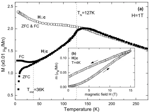
undoped LaSrMnO ₄ has been inves- tigated in detail by several groups [7, 42, 43, 46, 49, 50]. Below T _N ≈ 128 K the compound orders antifer- romagnetically as evidenced by the appearance of superstructure reec- tions with propagation vector Q = ( ¹ / 2 1 / 2 0) in neutron scattering exper- iments. The magnetic moments are aligned along the tetragonal c -axis, and at low temperatures the ordering is three dimensional and long range.

Due to the antiferromagnetic order- ing within the planes, the coupling between neighboring planes is frus- trated in the body-centered K ₂ NiF ₄ structure, and two dierent twin do-

mains corresponding to the two ordering schemes shown in Fig. 3.3 contribute

in diraction experiments. Next-nearest neighbor planes are coupled ferromag-

netically via a weak higher-order process yielding the three-dimensional G-type

arrangement. At low temperatures, the ordered moment is quite large, 3.21 µ _B ,

but still lower than 4.0 µ _B expected for a Mn ³⁺ -ion without an orbital contribution,

and the reduction of the ordered moment can only partially be explained by the

(30)

0 50 100 150 200 250 0.5

1.0 1.5 2.0 2.5

T stat

=36K H c

M(x0.01 B

/Mn)

Temperature (K)

(a)

H c

ZFC & FC

FC

ZFC

T N

=127K

H=1T

0 5 10 15

0.00 0.05 0.10

m(B

/Mn)

m agnetic field H (T) (b)

H||c

T=4K

Figure 3.4: Macroscopic magnetization of LaSrMnO 4 Temperature dependence of the macroscopic magnetization M (T ) in LaSrMnO 4 for a eld H = 1 T applied parallel and perpendicular to the c -axis. Upon eld cooling (FC), a nite magnetization is visible for H||c , while in the zero-eld run (ZFC) the magnetization vanishes for T → 0 K (a).

Field dependence of the magnetization M(H) at T = 4 K for the eld H applied along c revealing a nite remanent magnetization of ≈ 0.05 µ _B / Mn (b). All data were digitized from Ref. [43].

inuence of magnetic uctuations in the two-dimensional structure. The critical behavior close to the phase transition at T _N has been shown to resemble the char- acteristic behavior of a two-dimensional antiferromagnet with a strong Ising-like anisotropy, which furthermore is supported by a large anisotropy-gap in the mag- netic excitation spectrum, and LaSrMnO ₄ is treated as a simple two-dimensional Heisenberg antiferromagnet in the recent literature [7]. However, although the above picture seems consistent and agrees nicely with the proposed orbital order- ing in LaSrMnO ₄ , a careful analysis of the macroscopic magnetization and of the magnetic excitation spectrum are contrasting this simple approach and the actual situation is more complex [43, 46].

Macroscopic magnetization of LaSrMnO 4 In Fig. 3.4 we show the tempera-

ture and eld dependence of the macroscopic magnetization M (T, H ) as reported

by P. Reutler [43]. In a wide temperature regime the magnetization M(T ) ex-

hibits the typical behavior of a conventional antiferromagnet with the moment

aligned along c above T _N = 128 K M (T ) shows a Curie-like increase and below

(31)

3.1 Basic properties of single-layered LaSrMnO 4

the Néel transition the parallel magnetization M _|| (T ) with the eld H applied parallel to the ordered moment decreases, while the perpendicular magnetization M ⊥ (T ) is only slightly aected due to the induced canting of the spins. However, at low temperatures T < 40 K the progression of M _|| (T ) signicantly deviates from the expected behavior of a simple antiferromagnet: While M || (T ) vanishes for T → 0 K in the zero-eld cooled (ZFC) cycle, the eld-cooled (FC) signal shows a pronounced cusp at T _stat ≈ 36 K and the magnetization remains at a nite value of ≈ 0.015 µ _B / Mn for T → 0 K . A similar behavior is absent in the perpendicular magnetization and the low-temperature properties of the magne- tization M (T ) point to the existence of ferromagnetic domains, which can be aligned by a magnetic eld applied along c .

The eld dependence of the magnetization M(H) at T = 4 K further sup- ports the existence of ferromagnetic correlations. Below T _stat , for small elds H||c ^∂ _∂H ² ^M 2 > 0 , and M (H) is curved to the left, while M (H) is right-curved for strong elds H > 10 T , somehow reminiscent of a metamagnetic transition [61].

Furthermore, with decreasing eld a signicant hysteresis and a nite remanent magnetization ≈ 0.05 µ _B / Mn is observed, in strong contrast to the expected be- havior of an antiferromagnet with vanishing macroscopic magnetization in zero eld [43].

Magnon spectrum of LaSrMnO 4 The second experimental evidence against the simple Heisenberg ordering in LaSrMnO ₄ comes from the analysis of the spin- wave excitation spectrum. The magnon dispersion in the ordered phase has been investigated using inelastic neutron scattering by Larochelle et al. [7] and in the Diploma thesis of myself [46]. The q -dependence of the magnetic excitations along the main symmetry directions as elaborated in Ref. [46] is shown in Fig. 3.5.

Using cold neutrons, the energy scan at the antiferromagnetic zone-center Q = (0.5 0.5 0) reveals three dierent contributions to the excitation spectrum at ~ ω _cl,1 = 3.3 meV , ~ ω _cl,2 = 6.5 meV , and ~ ω _sw = 8.80 meV [46], ³ in contrast to the expectation of a single magnon branch in a two-dimensional Heisenberg model, see Fig. 3.5b. However, only the mode ω _sw possesses a pronounced q -dependence within the MnO ₂ -planes, see Fig. 3.5a, which is well describable following linear spin-wave theory. With only a nearest-neighbor exchange J _AFM in the layers, the Heisenberg model on a two-dimensional square lattice yields in linear approxima- tion the dispersion relation

~ ω = 4J _AFM S q

1 + α 2

− ¹ ₄ cos(2πq _h ) + cos(2πq _k ) 2

, (3.1)

with α = Λ/2J _AFM and the single-ion anisotropy Λ [62]. The observed q - dependence is excellently modeled using the parameter set J _AFM = 3.07 meV

3 Note, that Larochelle et al. only discuss a single magnon branch at 8.80 meV, although a

second feature at 6.5 meV is clearly resolvable in the data shown in Fig. 4 of Ref. [7].

Neutron Scattering Studies on Magnetic Excitations in Complex Ordered Manganites