Neutron-Scattering Studies on Chiral Multiferroics

Neutron-Scattering Studies on Chiral Multiferroics

Inaugural-Dissertation

zur

Erlangung des Doktorgrades

der Mathematisch-Naturwissenschaftlichen Fakult¨ at der Universit¨ at zu K¨ oln

vorgelegt von

Max Michael Baum

aus K¨ oln

K¨ oln, 2013

Vorsitzender

der Pr¨ ufungskommission: Prof. Dr. S. Trebst

Tag der letzten m¨ undlichen Pr¨ ufung: 5. Juli 2013

Abstract

Magnetoelectric multiferroics exhibit a strong correlation of magnetism and ferro- electricity. Among the multiferroics with a strong magnetoelectric effect many have a chiral antiferromagnetic structure. In these materials it is possible to con- trol the electric polarisation by an applied magnetic field and, inversely, to manip- ulate the antiferromagnetic domains by an applied electric field. The observation of antiferromagnetic domains requires a microscopic method, which neutron scat- tering with polarised neutrons is particularly suitable for. This thesis reports on neutron and X-ray measurements on several (chiral) antiferromagnetic multifer- roics. Special attention is devoted to the switching of (chiral) antiferromagnetic domains.

Neutron-diffraction data on the magnetic structures of the pyroxenes NaFeSi

O

and LiFeSi

O

are presented. LiFeSi

O

undergoes a single magnetic phase tran- sition below 18 K into a canted antiferromagnetic structure with the magnetic space group P 2

/c

. NaFeSi

O

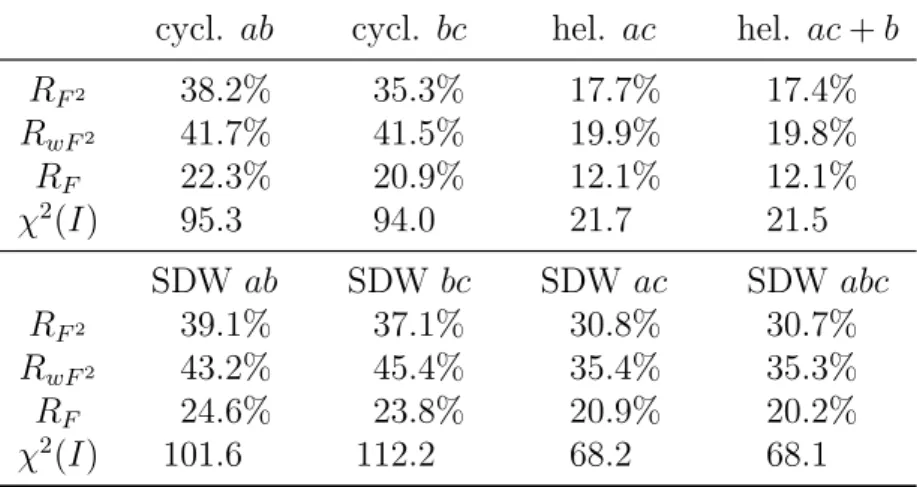
undergoes two magnetic phase transitions. Both phases are incommensurate with propagation vector k = (0, 0.77, 0). Below 8 K a transverse spin-density wave with moments in the ac plane sets in and below 6 K a helix with moments remaining in the ac plane evolves. By the use of spherical neutron polarisation analysis it is demonstrated that antiferromagnetic domains in LiFeSi

O

can be reversed by a combination of electric and magnetic fields. The magnetic structure of LiFeSi

O

gives rise to a toroidal moment. Therefore, the re- sults are discussed in the context of manipulating toroidal domains. Furthermore, the magnon dispersion and the spin density of LiFeSi

O

are presented.

In many chiral multiferroics it is possible to reverse the chirality of the mag- netic structure by an applied electric field providing the opportunity of driving hysteresis loops (chiral ratio vs. electric field). Results of the time dependence of this switching process in MnWO

studied by stroboscopic techniques for polarised neutron scattering reveal a surprisingly slow relaxation process in the time scale of 2 ms to 30 ms and a strong temperature dependence.

Furthermore, static hysteresis loops recorded on TbMnO

and DyMnO

are

reported. In TbMnO

, the coercive field increases linearly with decreasing tem-

perature. In DyMnO

, driving of hysteresis loops is possible only close to the ferro-

electric phase transition. Further investigations on TbMnO

show that the quasi-

lock-in of the magnetic propagation vector takes place at temperatures slightly

above the development of the chiral magnetic structure. In addition, the propa-

gation vector increases linearly with isotropic pressure. X-ray diffraction on single

crystals of TbMnO

and YMn

O

reveals that the deviation of the ions from their

centrosymmetric positions in the ferroelectric phase is beyond the resolution limit

of the performed diffraction experiments.

Kurzzusammenfassung

Magnetoelektrische Multiferroika sind gekennzeichnet durch eine starke Wechsel- wirkung magnetischer und ferroelektrischer Ordnung. Viele dieser Multiferroika mit starkem magnetoelektrischem Effekt bilden eine chirale, antiferromagnetis- che Magnetstruktur. In diesen Materialien ist es m¨ oglich, die elektrische Po- larisation mit einem ¨ außeren Magnetfeld, und umgekehrt, die antiferromagnetis- chen Dom¨ anen mit einem ¨ außeren elektrischen Feld zu schalten. Die Beobach- tung antiferromagnetischer Dom¨ anen ist nur mit einer mikroskopischen Methode zug¨ anglich, wof¨ ur sich Neutronenstreuung mit polarisierten Neutronen als her- vorragend geeignet erweist. Diese Arbeit handelt von Neutronen- und R¨ ongen- messungen an verschiedenen (chiralen) antiferromagnetischen Multiferroika. Das Schalten von (chiralen) antiferromagnetischen Dom¨ anen steht im Vordergrund der Untersuchungen.

Neutronendiffraktometrie liefert folgendes Bild von den Magnetstrukturen der Pyroxene NaFeSi

O

und LiFeSi

O

: In LiFeSi

O

gibt es einen magnetischen Phasen¨ ubergang bei 18 K unterhalb dessen eine verkantete, antiferromagnetische Ordnung mit magnetischer Raumgruppe P 2

/c

vorliegt. In NaFeSi

O

gibt es zwei magnetische Phasen¨ uberg¨ ange. Beide Phasen sind inkommensurabel mit Propagationsvektor k = (0, 0.77, 0). Unterhalb von 8 K setzt eine transversale Spindichtewelle mit magnetischen Momenten in der ac-Ebene ein, die sich un- terhalb von 6 K in eine helikale Struktur verwandelt, wobei die Momente in der ac-Ebene bleiben. Sph¨ arische Neutronenpolarisationsanalyse zeigt, dass antifer- romagnetische Dom¨ anen in LiFeSi

O

mit einer Kombination von elektrischen und magnetischen Feldern ausgerichtet werden k¨ onnen. Die Magnetstruktur in LiFeSi

O

ist toroidal. Daher werden die Ergebnisse im Zusammenhang mit der Ausrichtung toroidaler Dom¨ anen diskutiert. Zus¨ atzlich werden die Magnonendis- persion und die Spindichte von LiFeSi

O

besprochen.

In vielen chiralen Multiferroika kann die Chiralit¨ at der Magnetstruktur durch das Anlegen eines elektrischen Feldes umgekehrt werden. Dies erm¨ oglicht das Aufnehmen von Hysteresekurven (chirales Verh¨ altnis gegen elektrisches Feld). Die Untersuchung der Zeitskala dieses Schaltprozesses in MnWO

mit stroboskopis- cher, polarisierter Neutronenstreuung zeigt ein ¨ uberraschend langsames Schaltver- halten im Bereich von 2 ms bis 30 ms und eine starke Temperaturabh¨ angigkeit.

Des weiteren werden statische Hysteresekurven an TbMnO

und DyMnO

gezeigt. In TbMnO

nimmt das Koerzitivfeld linear mit fallender Temperatur

zu. In DyMnO

k¨ onnen Hysteresezyklen nur in der N¨ ahe des ferroelektrischen

Phasen¨ ubergangs durchlaufen werden. Weitere Untersuchungen an TbMnO

zeigen, dass der quasi-lock-in des magnetischen Propagationsvektors knapp ober-

halb des Einsetzens der chiralen magnetischen Ordnung stattfindet. Der Prop-

der Ionen aus ihrer zentrosymmetrischen Lage in der ferroelektrischen Phase sehr

gering ist und unterhalb des Aufl¨ osungsverm¨ ogens der durchgef¨ uhrten Messungen

liegt.

Contents

Abstract 3

Kurzzusammenfassung 5

1 Multiferroics 9

2 Polarised Neutron Scattering 15

2.1 The Structure Factor . . . . 15

2.1.1 Magnetic Scattering . . . . 16

2.2 Polarised Neutron Scattering . . . . 17

2.2.1 Chiral Magnetic Structures . . . . 21

2.2.2 The Flipping Ratio . . . . 23

2.2.3 History of Polarised Neutrons . . . . 24

2.3 Polarised Neutron-Scattering Technique . . . . 25

2.3.1 Polarising the Neutron Beam . . . . 25

2.3.2 Guiding the Polarised Neutron Beam . . . . 27

2.3.3 Spin Flippers . . . . 28

2.3.4 CRYOPAD . . . . 29

2.4 Time-Resolved Neutron Scattering . . . . 30

2.5 Linear Spin-Wave Theory . . . . 31

3 LiFeSi

O

35 3.1 Magnetic structure . . . . 36

3.2 Poling of Antiferromagnetic Domains . . . . 39

3.2.1 Experimental . . . . 42

3.2.2 Discussion . . . . 51

3.3 Toroidal Moment . . . . 52

3.4 Spin Waves . . . . 57

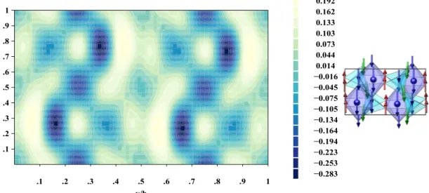
3.5 Spin Density . . . . 60

3.6 Conclusion . . . . 64

4 NaFeSi

O

65 4.1 Samples . . . . 66

4.2 Symmetry Analysis . . . . 67

4.3 Spherical Polarisation Analysis at IN14 . . . . 69

4.4 Single-Crystal Measurement at D10 . . . . 72

4.4.1 Crystal Structure . . . . 72

4.4.2 Magnetic Structure . . . . 73

4.5 Natural Powder Sample at G4.1 . . . . 74

4.6 Synthetic Powder Sample at G4.1 . . . . 79

4.7 Pressure at 4F2 . . . . 82

4.8 Conclusion . . . . 84

5 MnWO

87 5.1 Time-Dependent Measurements at IN12 . . . . 89

5.2 Time-Dependent Measurements at IN14 . . . . 97

5.3 Conclusion . . . . 101

6 TbMnO

103 6.1 Quasi-lock-in of the Propagation Vector . . . . 105

6.2 Hysteresis . . . . 106

6.3 Pressure . . . . 110

6.4 X-Ray Crystal-Structure Analysis . . . . 113

6.5 Conclusion . . . . 116

7 DyMnO

117 7.1 Hysteresis . . . . 118

7.2 Conclusion . . . . 120

8 YMn

O

121

9 Conclusion 127

Bibliography 131

Danksagung 141

Erkl¨ arung 143

1 Multiferroics

As the term multiferroics already reveals, it refers to materials which combine several ferroic properties. The three ferroic properties are ferroelectricity, ferro- magnetism, and ferroelasticity. A material is called multiferroic if two or all three of these properties occur simultaneously in the same phase [1].

A ferroic material is characterised by the fact that it forms domains which ex- hibit a macroscopic property (e.g. magnetisation) which in turn interacts with a related field and by means of this field can be reversed. A ferromagnetic ma- terial possesses a spontaneous magnetisation M

that can be switched by an applied magnetic field H. A ferroelectric material possesses a spontaneous elec- tric polarisation P

that can be switched by an applied electric field E. A ferroelastic material displays a spontaneous deformation that can be reversed by an applied mechanical stress [2]. Often the definition of multiferroics is expanded to include antiferromagnetic order which is characterised by ordered magnetic moments which cancel out each other on a microscopic scale and thus prevent a macroscopic magnetisation [3].

The topic of multiferroics gets exciting when the different order parameters do not just coexist but also interact with each other. Nowadays most attention is paid to the magnetoelectric coupling which describes the influence of a magnetic field on the electric polarisation P and vice versa the influence of an electric field on the magnetisation M . Up to the linear order this relation is given by

P

(E, H) = P

+

χ

E

+ α

H

+ . . . µ

M

(E, H) = µ

M

+ µ

χ

H

+ α

E

+ . . .

Whereas the electric and the magnetic susceptibilities χ

are symmetric the mag- netoelectric tensor α

is not [4, 5].

The term multiferroics is used predominantly for magnetoelectric multiferroics neglecting ferroelasticity. In spite of this the coupling between ferroelectricity and ferroelasticity – i.e. piezoelectricity – was already discovered in 1880 by J. and P. Curie [6] and has found indispensable technical application in electric cigarette lighters, in microphones, and as actuators in atomic force and scanning tunneling microscopes, to name just a few [7].

The magnetoelectric effect on the contrary – even though its existence was

pointed out by P. Curie in 1894 [8] – was predicted for Cr

O

not before 1959

by I. Dzyaloshinskii [9] and observed by D. Astrov in 1960 [10] and G. Rado

et al. (1961) [11]. Not much progress was reported on that topic from then until 2003 when research on magnetoelectric multiferroics regained substantial interest. This increase in interest has partly to do with the realisation how useful a magnetoelectric material with a strong magnetisation would be for applications [12–14].

Magnetoelectric materials are often discussed in the context of data storage.

Presently, most non-volatile data storage devices exploit the magnetisation of small grains for storing information. The magnetisation of these grains gets re- versed by a magnetic field. Generation of magnetic fields involves an electric current which consumes energy, produces heat, and is limited in size due to the coils carrying the current. Conversely, the generation of an electric field requires no constant current and solves all three problems at once. A magnetoelectric material with a sizeable magnetisation could then be used to be written by an electric field and read out by its magnetisation [15]. However, a suitable material has not yet been found. Most magnetoelectrics are antiferromagnets and have a low transition temperature. The reasons for that will be illuminated in the following.

Before moving on, it must be distinguished between single-phase and compos- ite multiferroics. Single-phase (magnetoelectric) multiferroics combine magnetic and ferroelectric properties intrinsically. Composite multiferroics consist of fer- romagnetic and ferroelectric phases which both have also a strong ferroelastic interaction. The magnetoelectric effect is mediated by the strain which is gener- ated in one phase by the application of an electric (magnetic) field and in turn causes magnetisation (polarisation) in the other phase. Regarding future appli- cations these composite multiferroics seem more promising. Anyhow, they are not topic of this thesis which entirely deals with single-phase multiferroics. Con- sidering fundamental physical concepts single-phase multiferroics are the more fascinating. These concepts will be recapitulated in the following [7].

Empirically, ferroelectricity and ferromagnetism seem to exclude each other.

The reason for that is found in the microscopic origin of both phenomena. In magnetic materials localised electrons of partly filled d or f shells of transition- metal or rare-earth ions form localised magnetic moments. Exchange interaction between these moments leads to their alignment. Ferroelectricity results from the relative shifts of positive and negative ions which breaks inversion symmetry. The microscopic origins for ferroelectricity are various [16, 17].

In classical ferroelectrics with perovskite structure (e.g. BaTiO

) the transition metal ion is located in the centre of an O

octahedron. The electric polarisation is caused by an off-centre shift of the transition metal ion with empty d shell in order to form covalent bonds with one or three of the surrounding oxygens.

Due to the empty d shell these ferroelectrics lack localised magnetic moments.

Introducing ions with partly filled d shells into such systems seems promising in

order to combine ferroelectricity and ferromagnetism (e.g. BiMnO

or BiFeO

).

However, the interaction of both order phenomena is weak [12, 13, 16].

The examples outlined above are so called proper ferroelectrics where structural instability towards the polar state, associated with electron pairing, is the cause of the ferroelectric transition. In improper ferroelectrics the ferroelectric transition is a consequence of a more complex lattice distortion or a byproduct of another type of ordering. An example for a complex lattice transition is the geometric ferroelectricity in hexagonal manganites (e.g. YMnO

) where the MnO

blocks tilt into the polar state. An example for another type of ordering is charge order in manganites (e.g. Pr

Ca

MnO

) where charges order non-centrosymmetric and induce electric polarisation [12, 16, 17].

Finally, electric polarisation can be induced by magnetic order. Obviously, strong magnetoelectric interaction can be expected for these compounds. Most of the magnetically induced multiferroics exhibit a spiral magnetic structure. The magnetic order in these systems is highly frustrated and competing interactions between the magnetic moments lead to complex magnetic structures. For that reason the order temperature in these compounds is rather low.

The most prominent representative of such systems is TbMnO

which was found to be multiferroic in 2003 [18]. This discovery marks the strong rise in enthusiasm for multiferroics. As in the case of TbMnO

, in many of these spiral multiferroics frustration leads to a sequence of magnetic phase transitions which start with a sinusoidal spin-density wave followed by the spiral phase. In the sinusoidal spin-density wave phase the moments are not completely ordered. With regard to minimising its entropy, the system has to find a way to order the remaining moments which may result in a spiral phase. In TbMnO

a sinusoidal spin-density wave sets in below 42 K and spiral order sets in below 28 K [19]. TbMnO

is further discussed in Chapter 6.

Observations of the magnetic phase transitions in different multiferroics (TbMnO

[19], MnWO

[20], Ni

V

O

[21], CuFeO

[22, 23]) confirm a sequence of two second-order magnetic phase transitions. While the first requires a sin- gle irreducible representation and is non-polar the second requires two irreducible representations and is polar. Only the second transition breaks the remaining symmetries and generates the ferroelectric phase [24]. NaFeSi

O

seems to be an exception of this rule as discussed in Chapter 4.

Spiral magnetic order is distinguished between helical and cycloidal arrange- ment of the magnetic moments. In a helical spiral the moments rotate in a plane perpendicular to the propagation vector while in a cycloidal spiral the propagation vector lies within the rotation plane of the spins. Both spirals break inversion sym- metry and may thus induce electric polarisation. A sinusoidal spin-density wave on the contrary does not break inversion symmetry and cannot induce ferroelec- tricity.

Among the spiral spin arrangements especially the cycloid is known to induce

ferroelectricity. The microscopic mechanism for that involves the antisymmetric

Dzyaloshinskii-Moriya interaction and was considered in References [25] and [26].

The Dzyaloshinskii-Moriya interaction between neighbouring moments is given by D

· S

× S

and favours non-collinear spin arrangement. The exchange in- teraction between neighbouring moments is usually mediated via super-exchange by oxygen ions forming bonds between pairs of transition metal ions. The bond angle determines the angle between the spins. In order to minimise the energy the Dzyaloshinskii-Moriya interaction can now inversely act on the bond angle and thereby shift the oxygens away from their centrosymmetric position. This mechanism is therefore called inverse Dzyaloshinskii-Moriya interaction. The dis- placement of the oxygen ions leads to electric polarisation which is given by

P ∝ X

ij

e

× (S

× S

) (1.1)

where e

points along the connection lines of the corresponding ions [17]. For the cycloidal spiral the connection line e

is perpendicular to the cross product S

× S

and a finite electric polarisation is induced. Cycloidal magnetic order can account for ferroelectricity in RMnO

(R = Tb, Dy, etc.) [19, 27, 28] (Chapter 6

& 7), MnWO

[29–31] (Chapter 5), Ni

V

O

[32] etc.

For the helical spiral e

is parallel to S

×S

and thus no polarisation is induced by the mechanism of Equation (1.1). Nevertheless there are examples of materials with helical magnetic structure which exhibit ferroelectricity, among them CuFeO

[23], Cu

Nb

O

[33], and NaFeSi

O

(Chapter 4). These compounds have in common that they have a rather low crystal symmetry (¯ 1 or 2/m). The helical magnetic structure further reduces the symmetry by breaking inversion and mirror operations. The only symmetry operations in accordance with helical magnetic structures are rotation axes. Electric polarisation is in accordance with rotation axes as long as the polarisation is parallel to them (polar axis). Once the symmetry operations which prevent the crystal from being ferroelectric are broken, the ions are prone shift into a polar state and ferroelectricity sets in [23, 33].

Another mechanism, which does not require spiral magnetic order and thus can account for ferroelectricity even in collinear spin arrangements, is the exchange striction. The energy between neighbouring spins is given by S

· S

. In a frus- trated magnetic structure the exchange striction shifts ions in a way to optimise their exchange energy. For example in a chain with nearest-neighbour ferromag- netic and next-nearest-neighbour antiferromagnetic interaction the moments with parallel spin will move closer together which may break inversion symmetry and generate electric polarisation [16, 17, 34]. Exchange striction is argued to be the predominant mechanism for ferroelectricity in YMn

O

[34, 35]. YMn

O

is dis- cussed in Chapter 8.

Considering the three well established ferroic properties under their behaviour

of the inversion of space and time gives the following picture. Ferroelasticity is

invariant against space and time inversion. Ferromagnetism is invariant against

space inversion but changes sign upon time inversion. Ferroelectricity changes sign upon space inversion but is invariant against time inversion. It is then a natural expansion to consider also a ferroic order parameter which breaks both space and time inversion. Ferrotoroidicity is claimed to be the fourth ferroic order parameter which fulfils the desired symmetry behaviour. The toroidal moment t of a bulk material with localised magnetic moments is given by the sum over all the magnetic moments m

and the cross product with their position vectors r

with respect to some origin

t = 1 2

X

α

r

× m

Naturally this quantity fulfils the desired symmetry behaviour. The ferrotoroidal state can be visualised as an array of spin vortices [36, 37].

Ferrotoroidal domains in a crystal are not necessarily identical to the antifer- romagnetic domains in the same crystal. A reversal of all magnetic moments in an antiferromagnetic domain however results in inversion of the toroidal moment.

Therefore it is questionable whether the toroidal moment can be considered as an independent ferroic state. In order to exhibit a toroidal moment a crystal must have an antiferromagnetic structure which additionally breaks inversion symme- try. Crystals with an antiferromagnetic structure known to give rise to a toroidal moment are LiCoPO

[38] and LiFeSi

O

(Chapter 3).

In magnetoelectric materials it is possible to manipulate the antiferromagnetic

structure by means of an electric field. Especially in materials with spiral mag-

netic structure it is possible to reverse the sense of rotation of the spiral [39]. A

microscopic method is required for observing antiferromagnetic domains. So far

two methods are available: optical second harmonic generation (SHG) [40] and

spherical neutron-polarisation analysis. The fundamentals of polarised neutron

scattering are reviewed in detail in Chapter 2.

2 Polarised Neutron Scattering

This chapter covers essential neutron-scattering formulas. Rather than giving a general introduction on the entire theory of neutron scattering, it is restricted to the formulas essentially used in this thesis. The main attention is thus directed to elastic polarised neutron scattering. General knowledge of scattering theory (i.e.

elementary X-ray scattering) is assumed.

The neutron-scattering experiments presented in this thesis have been per- formed at the Institut Laue-Langevin (ILL) in Grenoble, at the Laboratoire L´ eon Brillouin (LLB ) in Saclay (Paris), and at the Forschungsreaktor M¨ unchen II (FRM II) in Garching.

2.1 The Structure Factor

For elastic neutron scattering the length of the wave vector is retained during the scattering event k

= k

=

, i.e. the neutrons do not gain or yield energy to the crystal. The scattering vector is defined as the momentum transfer on the crystal due to the scattering process

Q = k

− k

(2.1)

Q = 4π

. Constructive interference is achieved only when the scattering vector is equal to a reciprocal lattice vector G

Q = G (2.2)

Equations (2.1) and (2.2) yield the Bragg equation 2k · G = G

which is commonly written as

2d sin θ = nλ

The intensity of the scattered neutrons I is proportional to the absolute square of the structure factor N . The nuclear structure factor N is the Fourier transform of the nuclei distribution, it is given by

N (Q) = X

j

b

e

e

The sum runs over all nuclei j in the unit cell of the crystal. b is the coherent scattering length of the corresponding nucleus which is in the range of 1 to 10 fm.

All values are listed in [41, 42]. The scattering length of an element depends on the isotope and on the orientation of the nuclear spin with respect to the neutron’s spin. It is a reasonable assumption that isotopes and nuclear spin are distributed randomly. They can therefore not contribute to the interference effect which assumes perfect periodicity of the scattering centres. The coherent scattering length b

is the mean value of the scattering lengths of the element averaged over the various possible isotopes and spin orientations. The uncorrelated distribution of the isotopes and the spins contributes to the so called incoherent scattering which is isotropic (i.e. it is independent of Q). Thus it adds to the background uniformly and can be neglected for most neutron-scattering experiments.

The Debye-Waller factor e

= exp(−

) = exp(−B

) = exp(−

) describes the effect of thermal motion on the intensity of the coherent scattering.

There are two common expressions for the temperature factor which are related by B

= 8π

U

. Thermal fluctuations of the nuclei about their equilibrium position diminish the intensity of the scattered neutrons. But where do these neutrons go?

They must still exist because the amount of incident neutrons must equal the amount of final neurons except for absorption due to neutron capture. Due to the statistical nature of the thermal fluctuations the crystal structure deviates from its periodic alignment. As in the case of incoherent scattering by the different isotopes and spins the thermal motion contributes to the background uniformly.

2.1.1 Magnetic Scattering

In analogy to the nuclear structure factor the magnetic structure factor for non- modulated structures (i.e. propagation vector k = 0) is given by

M (Q) = p X

j

f

(Q) m

e

e

The magnetic form factor f

(Q) represents the magnetisation distribution within a single magnetic ion. Its values are listed in [41, 42]. m is the mag- netic moment in units of µ

. The constant p = 2.695 fm/µ

relates the scattering length for a single magnetic moment of 1 µ

at Q = 0 to the nuclear scattering length b which is in the range of 1 to 10 fm. Therefore magnetic scattering is of the same magnitude as nuclear scattering or may eventually exceed it for large magnetic moments (∼ 10 µ

) as in rare earths. The magnetic interaction vector M

is the part of the magnetic structure factor M perpendicular to Q

M

= Q ˆ × (M × Q) ˆ (2.3)

Only that perpendicular part contributes to the scattered intensity. The intensity

is proportional to the absolute square of the magnetic interaction vector. When

2.2 Polarised Neutron Scattering

magnetic and nuclear scattering peaks occur in the same position (as they do for k = 0) the coherence between the magnetic and nuclear scattering amplitudes must be considered. In the case of unpolarised neutrons there is no coherence and the magnetic and nuclear intensities are additive.

I = |N |

+ |M

|

(2.4)

Modulated Magnetic Structures

For modulated structures (i.e. propagation vector k 6= 0) the formulas get slightly more complicated. The magnetic moment distribution m

can be Fourier ex- panded

m

= X

k

m

e

(2.5)

The Fourier components m

are in general complex vectors. The sum runs over all propagation vectors, usually k

= k and k

= −k. A necessary condition for the magnetic moments m

to be real is m

= m

, where

denotes complex conjugation. R

is the vector which translates the origin of the direct space to the individual unit cell of actual interest. The phase φ

= −φ

is not absolutely necessary. In principle any phase between two Fourier components can be deter- mined by the value of the components themselves. However, the equations become more intuitive when regarding two moments which are connected by symmetry.

In a centred cell for example the phase φ

= k · t relates the Fourier component of an ion to the one translated by the centering vector t.

Lastly, the magnetic structure factor for magnetic structures with propagation vector reads as

M (Q = G + k) = p X

j

f

(Q) m

e

e

This summary is based on text books [41–47].

2.2 Polarised Neutron Scattering

As mentioned earlier for unpolarised neutrons no coherence between magnetic and nuclear scattering has to be considered. In other words useful information can be gained by the use of polarised neutrons. Even when magnetic and nuclear scattering peaks do not occur in the same position (k 6= 0) useful information about the magnetic structure can be acquired by the use of polarised neutrons.

For a given axis of quantisation the neutron’s spin can be aligned either parallel

(+) or antiparallel (−). The polarisation of the neutron beam with respect to an

arbitrarily chosen axis (i = x, y, z) is then defined as P

= N

− N

N

+ N

(2.6) where N

is the number of neutrons with spin parallel to the axis i. In a completely unpolarised neutron beam there are equal amounts of both spin configurations, hence P = 0. A completely polarised beam has polarisation P = ±1.

It is useful to define a right handed, orthogonal coordinate system with respect to the scattering vector x k(−Q). z is chosen to be vertical on the scattering plane and y = z × x completes the right handed system. The usefulness of this definition becomes immediately obvious when regarding the magnetic interaction vector which now writes as M

= (0, M

, M

)

.

The polarisation of the incident neutron beam along some arbitrary axis is given by P = (P

, P

, P

)

. The scattered intensity under the condition that the incoming neutron beam is polarised is

I = N N

+ M

· M

+ P · M

N

+ P · M

N − iP · (M

× M

) (2.7) For unpolarised neutrons (P = 0) Equation (2.7) results in Equation (2.4).

In the most general case one is interested in the polarisation P

of the scattered intensity I

along some axis j under the condition that the incident neutron beam was polarised along i. Likewise to Equation (2.6) the scattered polarisation is defined as

P

= I

− I

I

+ I

(2.8) and P

= (P

, P

, P

)

. The sum (I

the scattered intensity when incident polarisation is parallel i)

I

= I

+ I

(2.9)

must hold as the neutron spin must be either up or down. Equation (2.8) and Equation (2.9) yield

I

= 1

2 (I

+ P

I

) (2.10) which is a useful expression once P

I

is available. This quantity is in fact given by

P

I = P (N N

− M

· M

)

+ M

(P · M

) + M

(P · M

) + M

N

+ M

N

− iP × (M

N

− M

N ) + i(M

× M

)

(2.11)

Equations (2.7) and (2.11) are called the Blume-Maleev equations. They

were derived simultaneously and independently by the physicists M. Blume and

2.2 Polarised Neutron Scattering

S. Maleev et al. in the early 1960’s [48, 49]. However, for better understanding an article of P. J. Brown [50] is recommended. Table 2.1 summarises all of the 36 possible channels of neutron-polarisation analysis. The different contributions are classified depending on their origin as nuclear, magnetic, chiral magnetic and nuclear magnetic interference term.

Two simple rules which in many cases are sufficient and provide greater insight can be deduced from the complete set of equations: (I.) Components of the mag- netic moment which are parallel to the neutron polarisation produce non-spin-flip scattering, while those perpendicular to the neutron polarisation produce spin-flip scattering. (II.) Hence, if the neutron polarisation is along the scattering vector, all magnetic scattering is spin-flip scattering [51].

It is useful to summarise the polarisations in a matrix-like notation

P

= (P

, P

, P

) =





P

P

P

P

P

P

P

P

P



 (2.12)

with P

as columns. Note that just 18 of the intensity channels contribute to this

kind of matrix.

Neutron Scattering

xx = N N

x¯ x = M

· M

− i(M

× M

)

¯

xx = M

· M

+ i(M

× M

)

¯

x¯ x = N N

yy = N N

+ M

M

+ 2<(M

N )

y¯ y = M

M

¯

yy = M

M

¯

y¯ y = N N

+ M

M

− 2<(M

N )

zz = N N

+ M

M

+ 2<(M

N )

z z ¯ = M

M

¯

zz = M

M

¯

z z ¯ = N N

+ M

M

− 2<(M

N )

xy = y¯ x =

/

(N N

+ M

· M

− i(M

× M

)

+ 2<(M

N ) + 2=(M

N )) x¯ y = ¯ y¯ x =

/

(N N

+ M

· M

− i(M

× M

)

− 2<(M

N ) − 2=(M

N ))

¯

xy = yx =

/

(N N

+ M

· M

+ i(M

× M

)

+ 2<(M

N ) − 2=(M

N ))

¯

x¯ y = ¯ yx =

/

(N N

+ M

· M

+ i(M

× M

)

− 2<(M

N ) + 2=(M

N )) xz = z x ¯ =

/

(N N

+ M

· M

− i(M

× M

)

+ 2<(M

N ) − 2=(M

N )) x¯ z = ¯ z x ¯ =

/

(N N

+ M

· M

− i(M

× M

)

− 2<(M

N ) + 2=(M

N ))

¯

xz = zx =

/

(N N

+ M

· M

+ i(M

× M

)

+ 2<(M

N ) + 2=(M

N ))

¯

x¯ z = ¯ zx =

/

(N N

+ M

· M

+ i(M

× M

)

− 2<(M

N ) − 2=(M

N )) yz = zy =

/

(N N

+ M

· M

+ 2<(M

M

) + 2<(M

N ) + 2<(M

N )) y¯ z = ¯ zy =

/

(N N

+ M

· M

− 2<(M

M

) + 2<(M

N ) − 2<(M

N ))

¯

yz = z y ¯ =

/

(N N

+ M

· M

− 2<(M

M

) − 2<(M

N ) + 2<(M

N ))

2.2 Polarised Neutron Scattering

2.2.1 Chiral Magnetic Structures

The concept of chirality is most intuitively introduced by considering human hands (Greek: χιρ, hand). The mirror image (enantiomorph) of the right hand is the left hand and it is not possible to bring both hands to coincident by the use of pure rotation or translation operations. Lord Kelvin introduced the term chirality in 1904. Generally an object can be defined to be chiral, if it is not superposable by pure rotation or translation on its mirror image [53].

Chirality is an important property in nature. Enantiomers (enantiomorphs of molecules) often smell and taste differently.

An object is chiral, if its point group contains no symmetry elements like inver- sions (¯ 1), mirrors (m), and rotoinversions (¯ n). The point group must contain only pure rotations (n). Chirality depends on the dimension of the space. A chiral object in two dimensions, such as the palm of the hand, becomes achiral in three dimensions, since the plane containing the two-dimensional object becomes then a mirror symmetry.

Before we move on to chirality of magnetic structures we must consider the ac- tion of symmetry operations on magnetic moments. We can imagine a magnetic moment as an infinitesimal current loop. Time inversion (1

) will therefore reverse the direction of the current and thus the direction of the magnetic moment. In an analogous manner we can investigate how the current loop reacts on spatial sym- metry operations. This is a tedious exercise. The results can best be summarised by introducing the concept of polar and axial vectors. For this purpose we write the symmetry operation as an orthogonal 3 × 3 matrix. The symmetry opera- tions can then be classified as proper, det(α) = 1 (real rotation), and improper, det(α) = −1 (inversion, refection). When the vector is polar (e.g. the electric dipole moment) it transforms as g(p) = α · p. When the vector is axial (e.g. the magnetic dipole moment) it transforms as g(a) = det(α) α · a.

The complexity of the term chirality comes along when considering dynamical aspects (here current loops i.e. magnetic moments) as in the following example. A parallel arrangement of a magnetic and an electric dipole moment ↑

↑

seems to be a chiral object as both moments become antiparallel ↓

↑

under space inver- sion and are not superposable onto each other. However, the same configuration can be obtained, by time inversion combined with a two-fold rotation. The former given definition of chirality gives no clear answer how to deal with time inversion.

L. Barron introduces the term true chirality : True chirality is possessed by sys-

1

In crystallography (restricted to three dimensions) it is customary to define an object as chiral, if it is not superposable by pure rotation or translation on its image gained by inversion.

(The equivalence of both definitions becomes obvious when remembering that a mirror is a combination of a spatial inversion and a two-fold rotation, m = ¯ 2.)

2

If we do not distinguish any more between the palm of the hand and its back we can super-

impose the right and the left hand if we flip on hand.

tems that exist in two distinct enantiomeric states that are interconverted by space inversion but not by time reversal combined with any proper spatial rotation [54].

When dealing with magnetic structures we have an intuitive understanding of the sense of spin rotation. It is customary to associate this sense of spin rotation to some value. A suitable value is the vector chirality

χ = S

× S

determined by two consecutive spins S

and S

on an oriented path. The behaviour of the vector chirality will now be discussed in regard of two most prominent magnetic structures with a sense of rotation: the helical and the cycloidal magnetic structure.

Helical magnetic structure means the propagation vector is perpendicular to the plane of rotation of the magnetic moments so that the connection line of the magnetic moments forms a helix (also referred to as screw type magnetic structures). Space inversion produces two enantiomorphs with spins rotating in the opposite sense around the axis of the helix. Neither time inversion nor rotation about any axis does change the sense of spin rotation. Thus a helix shows true chirality according to Barron. The vector chirality for both enantiomorphs has opposite sign and is in accordance of our intuitive understanding.

Cycloidal magnetic structure means the propagation vector lies in the plane of rotation of the magnetic moments so that the connection line of the magnetic mo- ments forms a cycloid. Again, space inversion produces two configurations with spins rotating in the opposite sense in the plane. However a two-fold rotation about an axis either perpendicular to the rotation plane of the spins or parallel to the propagation vector produces the same configuration (modulo a translation).

Obviously, such an object is not chiral. This behaviour is a consequence of the cy- cloid being a two-dimensional object in three-dimensional space. Nevertheless it is possible to unambiguously assign distinct vector chiralities to both configurations.

An excellent review on chirality is given by V. Simonet, M. Loire, and R. Ballou [55].

In many multiferroic materials with spiral magnetic structure

the microscopic origin of the ferroelectricity is the inverse Dzyaloshinskii-Moriya interaction. The direction of the electric polarisation P is given by P ∝ P

ij

e

× (S

× S

) where S

and S

are the magnetic moments of neighbouring magnetic ions and e

points along the connection line of the corresponding ions.

3

Spiral magnetic structure is used as a collective term for helical, cycloidal and mixed types

of spin arrangements.

2.2 Polarised Neutron Scattering

We recognise the term S

× S

as the vector chirality. It is non-zero only for non-collinear spin arrangements. In particular sinusoidal spin-density waves yield a vanishing cross product of neighbouring magnetic moments.

Neutron scattering with polarised neutrons suggests itself for studying magnetic structures with a non-vanishing term S

× S

as it gives access to the so called chiral term: −i(M

× M

)

. The chiral ratio is defined as

r

= −i(M

× M

)

|M

|

As we learn from Table 2.1 the chiral ratio can be measured likewise in several channels of the neutron polarisation. The strongest intensity can be detected in the channel I

= |M

|

− i(M

× M

)

and I

= |M

|

+ i(M

× M

)

:

r

= I

− I

I

+ I

(2.13)

In order to observe the chiral term and the chiral ratio the scattering vector must have a component perpendicular to the rotation plane of the magnetic moments.

Only if the scattering vector is exactly perpendicular to this rotation plane chiral ratios of ±1 are possible

2.2.2 The Flipping Ratio

When undertaking a neutron-scattering experiment with polarised neutrons the quality of the polarisation of the incoming beam is an important factor as all scattering results will depend on it. The polarisation was given by Equation (2.6):

P

=

i+N¯i

. A polarisation of 1 is desired yet experimentally not obtainable, of course. So N

represents the number of the ’good’ neutrons whose spin is aligned properly while N

represents the number of the ’bad’ neutrons whose spin is misaligned. Another frequently used quantity is the flipping ratio which is defined as

FR = N

N

The flipping ratio and the polarisation are connected by the following relations:

FR = 1 + P

1 − P P = FR − 1 FR + 1

Under good experimental conditions a flipping ratio of 40 is readily achieved, but at 20 reasonable results still can be obtained (polarisation of ∼ 0.95 and ∼ 0.90, respectively).

4

Proof: In our notation Q k(−x). Imagine an arbitrary spiral magnetic structure with the

scattering vector in the plane of rotation of the magnetic moments. Without loss of generality

we choose M = M

x + M

y. Obviously M

= M

y. It follows M

× M

= 0. Now let

the scattering vector be perpendicular to the plane of rotation: M = M

y + M

z. It follows

M

= M

y + M

z, but now M

× M

= (M

M

− M

M

)x.

2.2.3 History of Polarised Neutrons

The existence of the neutron was predicted by E. Rutherford in 1920 in order to explain the nuclear constitution of atoms [56]. The neutron was proposed as a neutral particle consisting of close combination of a proton and an electron. A concept which was elaborated in the theory of β decay of the neutron by E. Fermi in 1934 [57]. It was J. Chadwick who experimentally verified its existence in 1932 [58, 59]. Although since its discovery it was generally accepted that the neutron is a spin-

/

particle [60, 61] it lasted till 1947 until an unambiguous experimental proof was delivered [62]. The magnetic moment of the neutron was postulated already in 1934 [63]. In 1936, short after their discovery, it was shown that neu- trons could be diffracted by crystals [64]. It was the same year when F. Bloch pointed out that neutrons will scatter from an atom not only on account of the interaction of the neutron with the atomic nucleus but also on account of the inter- action of the neutron’s magnetic moment with the magnetic moment of the atom [65]. In 1937 J. Schwinger gave a more detailed theory on an unpolarised beam of neutrons which will be partially polarised after being transmitted through a fer- romagnet [66]. Experimentally this was accomplished 1938 [67, 68]. O. Halpern and M. Johnson advanced the theory of magnetic neutron scattering and placed special emphasis upon questions of polarisation (1937-1939) [69–71]. Again, Bloch together with L. Alvarez determined the magnetic moment of the neutron by po- larisation analysis in 1940 [72]. The first determination of a magnetic structure was carried out in a pioneering experiment by C. Shull and J. Smart in 1949 on antiferromagnetic MnO [73]. In 1951 complete polarisation of the neutron beam by reflection of neutrons from magnetised mirrors was reported [74]. In the same year complete polarisation by Bragg scattering on antiferromagnetic magnetite (Fe

O

) was achieved by Shull et al. [75]. In 1959 the first measurement with po- larised neutrons was carried out and the magnetic form factors of nickel and iron were determined [76, 77]. In this experiment the incident neutron beam was po- larised either parallel or antiparallel to the magnetisation of the scattering crystal and the corresponding intensities were compared. A general theory of polarised neutron scattering was published simultaneously and independently by the physi- cists M. Blume and S. Maleev et al. in 1963 [48, 49]. In contrast to the former theory by Halpern and Johnson, which was restricted to ferromagnetic and simple antiferromagnetic structures, no restrictions were made. As a consequence inter- esting polarisation effects in the case of scattering by spiral spin structures were henceforth computable.

In 1969 the development of the first triple-axis spectrometer with uniaxial (lon- gitudinal ) polarisation analysis was reported by R. Moon, T. Riste and W. Koehler [51]. They installed a polariser before and polarisation analysis behind the sample.

The direction of polarisation could be chosen to be perpendicular or parallel to

the scattering vector. Due to the need of a continuous magnetic guide field from

2.3 Polarised Neutron-Scattering Technique

the polariser to the analyser the polarisation and analysis were always parallel or antiparallel, hence the term uniaxial. The instrument allowed to choose the spin state of the incident beam to be (+) or (−) and equally the spin state of the scattered beam to be (+) or (−). This way for either polarisation axis (P ⊥ Q or P k Q) four scattering amplitudes were available.

The guide field is necessary to preserve the neutron polarisation. Without guide field small fields as the earth’s magnetic field will disturb the original polarisation of the beam as the neutron spin will precess about the field direction leaving only the component along the field observable. As Moon et al. [51] already point out, observing the scattered polarisation not in the direction of the incident polari- sation, would require a magnetic field which changes direction precisely at the location of the scattering centre. This is of course unfeasible. Another solution to overcome this challenge is to install a zero-field chamber at the position of the scattering centre. The first sophisticated experimental realisation was presented by F. Tasset in 1989 [78]. The CRYOPAD (cryogenic polarisation-analysis device) makes use of superconducting Meissner screens to expel any magnetic field from the scattering centre. The guide fields before and after the scattering centre can thus be selected independently. This way any arbitrary spin state for the incident and the scattered beam can be achieved. In comparison to the former methods this technique represents a great improvement. For the first time all polarisation channels summarised in Table 2.1 were available. That is why this method is referred to as spherical (vectorial, three-dimensional ) polarisation analysis. The setup of CRYOPAD is described in detail in Section 2.3.4.

This historical overview follows a lecture of R. Stewart [79] and an article of J. Schweizer [80].

2.3 Polarised Neutron-Scattering Technique

2.3.1 Polarising the Neutron Beam

There are three different methods of polarising the neutron beam which will be described in the following.

Polarising Crystals

Ferromagnetic single crystals can be used to simultaneously polarise and

monochromatise the neutron beam. A magnetic field is applied along the crystal

perpendicular to the scattering vector to saturate the magnetic moments along

the field direction. For an unpolarised beam P = 0 the Blume-Maleev equations

(2.7) and (2.11) yield

P

= 2M

N

|N |

+ |M

|

= 2M

N

|N |

+ |M

|

z

The chiral term −i(M

× M

)

is zero for collinear structures. For centrosym- metric and for simple collinear magnetic structures N and M

are real quantities.

If the magnetic field aligns all moments along the z direction then M

= M

z.

Under the special condition that the nuclear and the magnetic scattering ampli- tude are of the same magnitude the neutron beam is completely polarised and by reversing the magnetic field it is possible to reverse the neutron polarisation.

Suitable crystals are iron single crystals with a special amount of

Fe and the following alloys Co

Fe

, Cu

MnAl (Heusler) and Fe

Si. [79, 81]

Polarising Mirrors

For small scattering angles neutrons experience refraction. The refractive index n of a material is usually slightly smaller than 1 (e.g. 1 − n = 1.5 · 10

for Ni at λ = 1 ˚ A). From this it follows that neutrons can experience total reflection at the boundary between the material and the vacuum for very small incident angles, typically 0

10

. This effect facilitates the construction of neutron guides which allow to transport the neutrons from the reactor to the spectrometer without loss of intensity. By slightly bending the guide it is even possible to eliminate neutrons of higher energy and gamma rays.

For a ferromagnetic material the critical angle differs for both spin states. By choosing a suitable angle it is indeed possible to suppress one spin state and produce a completely polarised beam. Due to the small angle of total reflection a mirror must be a few meters long to produce a beam of a reasonable width.

More practical polarisers can be constructed by alternating several layers of magnetic and non-magnetic material. This way it is possible to tune the critical angle.

A polariser for broader wavelength range can be constructed if these bilayers exhibit a gradient in their thickness. These devices are called supermirrors. Typ- ically they are made from layers of Fe/Si or Co/Ti. To ensure that the neutrons are reflected at least once, the mirror can be gently bent. This device is then called a bender. Polarising multilayers produce a beam of high polarisation. The wavelength is restricted to exceed 2 ˚ A however. [44, 79, 81]

Polarising Filters

Polarising filters have different transmissibility for the two spin states. This is on

account of either preferential absorption or preferential scattering. The intensity

is a trade-off between attenuation and polarisation. Although in principle there

2.3 Polarised Neutron-Scattering Technique

are different isotopes which exhibit this feature the only one of contemporary interest is

He because it exhibits the strongest difference in the absorption cross- section for the two spin states. One spin state goes through the gas with strong absorption while the other one is less absorbed. The

He nuclei can be polarised by optical pumping using high power lasers, followed by compression of the gas.

Due to collisions with the walls of the container and stray magnetic fields the polarisation of the gas decreases over time. For transport and at the instrument magnetic shielding is employed. Nevertheless the cells have to be replaced about once a day. Usual polarisation for recharged cells is about 0.8. [81]

2.3.2 Guiding the Polarised Neutron Beam

For any experimental implementation utilising polarised neutrons, the action of a magnetic field on the magnetic moment of the neutron has to be taken into account. The magnetic moment of the neutron is given by µ

= γ

s where the gyromagnetic ratio of the neutron is γ

= −2 · 1.91 µ

/ ~ = −1.83 · 10

/sT.

µ

= e ~ /2m

= 5.05 · 10

J/T is the nuclear Bohr magneton. The relation of the nuclear Bohr magneton to the (electron) Bohr magneton is µ

= µ

/1836.

The z component of the neutron magnetic moment amounts µ

= γ

~ /2 =

−1.91µ

= −9.66 · 10

J/T. The relation of the neutron magnetic moment to the electron magnetic moment is µ

= µ

/961. [82, 83]

A magnetic field B exerts a torque T on the magnetic moment, T = µ

× B.

The time evolution of the spin is thus governed by the following equation ds

dt = γ

s × B

When the spin and the field are parallel in the beginning, the cross product is zero and the spin is preserved. Therefore such a field is called guide field. In the other case the spin precesses about field what can be seen from the general solution of the equation of motion

s(t) =





s

cos(ω

t) + s

sin(ω

t) s

sin(ω

t) + s

cos(ω

t)

s





with B = Be

and the Larmor frequency ω

= γ

B.

A guide field is needed to preserve the spin of the neutron. If the guide field rotates slowly in space (mathematical this means ω

/ω

1 where ω

is the rotation of the magnetic field, experimentally this can be accomplished by ω

/ω

> 10) the spin of the neutron will follow the guide field. This is called adiabatic rotation. On the other hand if the guide field changes non-adiabatically (i.e. ω

/ω

1) the spin begins to precess about the new field direction

[50, 80].

5

The calculation for the adiabatic and non-adiabatic rotation is not provided here.

So far the mathematical treatment was for a classical spin. For a quantum mechanical spin just one component of the spin is preserved, whilst the other components remain fluctuating. The classical analysis keeps valid however if the former spin is associated with the one component of the spin which is preserved.

The quantum mechanical spin comes along with some counterintuitive features.

One easy task is to imagine a neutron whose spin is aligned along the z direction and now will be measured along the y direction. As mentioned before a quan- tum mechanical spin can have only one fixed component. Subsequently when measuring this spin along the y direction its probability of the being parallel or antiparallel y is 1/2 each.

Mathematically the probability P

(y) of finding a spin being prepared in |zi along the y direction is given by the projection P

(y) = |hy|zi|

. In order to cal- culate this probability we must represent the states |yi and |zi in the eigenvectors of their operators given by the Pauli matrices s

=

σ

σ

=

0 1 1 0

σ

=

0 −i i 0

σ

=

1 0 0 −1

With |yi =

2

−i 1

and |zi = 1

0

it follows P

(y) = |hy|zi|

=

.

2.3.3 Spin Flippers

Scattering experiments with polarised neutrons usually require turning the neu- tron spin in the desired direction. Different devices are available. Two of them shall be described here.

Mezei Flipper

The principle of operation of a Mezei Flipper depends on the neutron spin un- dergoing a well-defined number of Larmor precessions in a fixed magnetic field over a well-defined distance. On entering the magnetic coil of the Mezei flipper the neutron is exposed to a field perpendicular to the guide field. Because the transition to the new field is non-adiabatic the spin starts to precess about the perpendicular field. When it exits the flipping field after performing exactly one rotation of π the spin is flipped. It is then preserved by the guide field which it now opposes. Neutrons of different velocities spend different precession time inside the coil, hence Mezei flippers can be employed for monochromatic beams only. [79, 84, 85]

Current Sheet (Dabs Foil) Flipper

Originally a foil, more advanced a grid of closely aligned copper wires, is introduced

into the neutron beam in a way that the neutrons pass through the sheet. A strong

2.3 Polarised Neutron-Scattering Technique

current in the direction of the guide field through the sheet produces a magnetic field perpendicular to the guide field. Right on the two sides of the sheet the magnetic field lines are of opposite direction. Because the foil is thin the neutrons experience a non-adiabatic field change when transmitting the foil. Precession does not occur at that point as the fields are exactly opposing. The superposition of the guide field and the field of the foil generates an ample transition region. It is that region which adiabatically reverses the neutron polarisation. This kind of flipper is independent of the neutron velocity. [79, 84]

2.3.4 CRYOPAD

This section describes the setup of the CRYOPAD III (cryogenic polarisation- analysis device) for spherical polarisation analysis. Spherical polarisation analysis allows choosing the direction of the incident and the final polarisation indepen- dently and thereby gives access to the full polarisation matrix (2.12). The off- diagonal terms of the polarisation matrix yield valuable information on the nu- clear magnetic interference. For the experimental implementation it is necessary to separate the guide fields of the incident and the final neutrons by a zero-field chamber at the position of the scattering centre. The guide fields define the direc- tion of polarisation analysis and may be chosen independently. In the zero-field chamber at the scattering centre the orientation of the spin is maintained. For a precise measurement of the spin direction an abrupt (non-adiabatic) transition into the zero-field region is required. This is accomplished by superconducting Nd-Meissner screens at the beam level, Figure 2.1. In addition, the environmental

Figure 2.1: CRYOPAD III (cryogenic polarisation-analysis device) [86]