Symbolic dynamics and scattering theory for localized magnetic fields

for localized magnetic fields

Dissertation

zur Erlangung des Grades eines Doktors der Naturwissenschaften

der Fakultät für Mathematik der Technischen Universität Dortmund

vorgelegt von Frank Schulz

Dortmund, Oktober 2013

Introduction 1

1 Preliminaries 5

1.1 Principles of classical mechanics . . . . 5

1.2 Magnetic fields and the magnetic flow . . . . 8

1.3 Symplectic rigidity . . . . 12

1.4 Topological entropy . . . . 16

2 Scattering theory 19 2.1 The virial radius . . . . 20

2.2 Time decay in a simplified time-dependent magnetic field . . . . 25

2.2.1 Asymptotic velocity and asymptotic position . . . . 28

2.2.2 Wave transformations . . . . 32

2.3 Spatial decay in a time-independent magnetic field . . . . 53

2.3.1 Asymptotic velocity and asymptotic position . . . . 55

2.3.2 Wave transformations . . . . 59

2.4 Wave transformations on the cotangent bundle . . . . 66

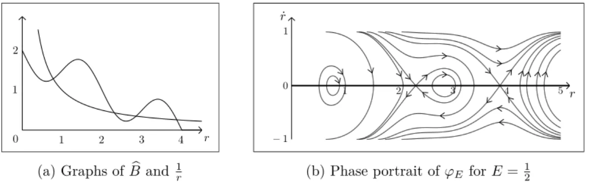
3 Symbolic dynamics 74 3.1 Rotationally symmetric magnetic fields . . . . 75

3.1.1 An additional integral of motion . . . . 75

3.1.2 Circular orbits and hyperbolicity . . . . 80

3.1.3 The motion outside the largest circular orbit . . . . 88

3.2 Symbolic dynamics for rotationally symmetric components . . . . 98

3.3 Non-rotationally symmetric magnetic fields . . . 109

3.3.1 The motion outside the largest circular orbit . . . 110

3.3.2 Symbolic dynamics for non-rotationally symmetric components . . 116

List of Symbols 123

Bibliography 124

Overview

The motion of a particle in a magnetic field has been object of research in many areas of mathematics, which include dynamical systems, mathematical physics, symplectic topo- logy, differential geometry and mathematical billiards. Some examples of the discussed topics are the interpretation of the magnetic flow as the geodesic flow of a non-reversible Finsler metric [8, 46], the comparison of magnetic and Riemannian geodesic flows [39]

and, most prominently, the question of the existence of closed orbits [9, 16, 30].

In this work, we shall focus on magnetic fields that vanish at infinity, which we summarize by the term “localized”. For the motion in these magnetic fields two types of orbits can occur: bounded and unbounded ones. The study of the unbounded orbits is the topic of scattering theory, while the bounded ones shall be examined by techniques of symbolic dynamics. In the following, we will give an introduction to these subjects and provide an outline of this work’s results.

The main goal in scattering theory is to study the asymptotic behaviour of the motion.

This theory has its origin in physics, where Rutherford’s scattering experiments with a gold foil gave rise to a new atomic model. The solid mathematical foundations were laid from the 1950s onwards, e.g. in [10], and much effort was devoted to scattering by a potential in the classical as well as in the quantum mechanical setting [21, 24, 44].

Scattering of a single classical particle in a non-constant magnetic field has, as far as we

know, only been treated by M. Loss and B. Thaller [33], who focused on the quantum

mechanical case of scattering in R

and considered the classical particle only for the

special case d = 3. Consequently, further studies have only been conducted for quantum

particles, see e.g. [34, 48]. The information about the asymptotic behaviour is contained

in so-called “wave transformations”. This allows the study of the inverse problem, i.e. the

reconstruction of the magnetic field from the asymptotic data, which is often called inverse scattering and has been treated by A. Jollivet for magnetic fields, e.g. in [26].

We will consider the motion of a classical particle and generalize the results obtained by M. Loss and B. Thaller to arbitrary dimensions d ≥ 2. Furthermore, we will extend them in the sense that we obtain stronger results for the regularity of the wave transformations, even for the case d = 3. In addition, we consider scattering in a simplified time-dependent magnetic field, which, to our knowledge, has not been studied before.

Symbolic dynamics is used to analyze dynamical systems by discretizing the underlying space. The key idea is to assign symbols to certain subsets of the space and label all trajectories by the successive visits of these sets. Then, the state of the dynamical system is described by an infinite sequence of symbols and the evolution is given by a shift map. These techniques have first been used by J. Hadamard in 1898 for the analysis of geodesic flows on surfaces of negative curvature [20]. Symbolic dynamics received its first formal treatment as well as its name in 1938 by G. Hedlund and M. Morse [38].

Their study of abstract symbolic systems was not only motivated by pure mathematical interest in these systems, it was also necessary to be able to use symbolic techniques for the study of continuous systems. However, the formal notion of shift spaces was first introduced in the 1960s by S. Smale, who contributed the most notable advancements to this theory [45]. One of the most important results involving the use of symbolic dynamics is Sharkovsky’s theorem about periodic points of continuous self-maps of an interval [42], but note that these techniques were not only used for the analysis of dynamical systems: The most prominent example is C. Shannon’s use of methods from symbolic dynamics for the mathematical foundation of communication theory, which has provided the basis for information theory [41]. For a more detailed presentation of the history of symbolic dynamics we refer to S. Williams’ article [47] as well as the book by D. Lind and B. Marcus [31].

Outline of the thesis

This work consists of three main sections.

First, in Chapter 1, we present preliminary results and gather necessary basics to perform

the analysis. We start by reviewing the foundations of classical mechanics, which are

Lagrange’s and Hamilton’s principles of motion and their connection by the Legendre

transformation. Based on this, we introduce the notion of a magnetic field and, in

particular, the notation we will use throughout this work. After this, we present a

deep result from symplectic topology, the symplectic rigidity. Although we will need it only once, due to its importance and complexity we outline the proof instead of simply quoting the theorem. Finally, we introduce the concept of topological entropy as a way to measure the complexity of a dynamical system.

In Chapter 2 we examine the unbounded orbits by using ideas of scattering theory, where it is the aim to compare the magnetic flow to the free flow. We start by considering a time-dependent magnetic field whose strength decays in time, which turns out to be easier to handle than spatial decay and will provide a useful tool for the calculations in the time-independent case. We consider the asymptotic velocity and the asymptotic position of the motion separately and then combine them to define the wave transformations, whose regularity depends on the rate of decay of the magnetic field. After that, we turn to time-independent magnetic fields which decay at infinity. Our main tool for their analysis will be the construction of a time-dependent magnetic field whose decay in time corresponds to the spatial decay of the original magnetic field. Using this and following the same plan as before, we obtain similar results for the regularity of the wave transformations. Finally, we consider the magnetic motion on the cotangent bundle where we also construct wave transformations. They turn out to be symplectic under certain assumptions, which is useful for fixed point problems like the question if there is an initial value with the same asymptotic velocity as the initial velocity.

Chapter 3 is devoted to the study of bounded orbits and focuses on symbolic dynamics.

In a magnetic field that consists of rotationally symmetric components, the question is if one can prescribe the itinerary of a trajectory, i.e. the order in which the components’

supports are visited. To answer this, we start by examining the motion in a single rotationally symmetric magnetic field. For sufficiently low energies, it admits circular orbits for which we analyze whether they are hyperbolic or elliptic. Furthermore, we find an integral of motion and use it to study the motion of trajectories that stay outside the largest circular orbit. For a magnetic field consisting of several rotationally symmetric components we choose a Poincaré section in each support and consider the corresponding Poincaré (first return) map. Using the results obtained for single components we show that the Poincaré map is semi-conjugated to the shift map. In particular, it has positive topological entropy and is chaotic. Finally, we show that the integral of motion is not necessary: The same result holds if we drop the assumption of rotational symmetry of the magnetic field.

Note that in Chapter 1 we present known results and concepts, while the ones we shall

obtain in Chapter 2 and Chapter 3 are new unless explicitly marked otherwise.

Acknowledgements

I am grateful to my advisor Prof. Dr. Karl Friedrich Siburg for suggesting this interesting

and fruitful topic to me and I would like to express my gratitude for his ongoing support

and advice. In particular, I am very thankful for him having established the contact to

Prof. Dr. Andreas Knauf, Prof. Dr. Mark Levi and Prof. Dr. Norbert Peyerimhoff: The

discussions we had have been very constructive and profitable. My thanks goes especially

to Prof. Levi and Prof. Peyerimhoff for their warm hospitality and their precious time

they spared for me during my stays. Last but not least I thank the German National

Academic Foundation for their financial support without which this work would not have

been possible.

Preliminaries

In this chapter, we are going to present basic results that are needed for the following considerations. In Section 1.1 we will give a short overview over the principles of classical mechanics. This is the basis for Section 1.2, the main part of this chapter, where we shall give the definition of a magnetic field and the magnetic flow. Furthermore, we will derive essential properties of the magnetic flow and introduce the corresponding notation we will constantly use. Afterwards, in Section 1.3 and Section 1.4, we are going to present two concepts, symplectic rigidity and topological entropy, that are required at certain points. However, they are rarely needed, while the notion of a magnetic field is essential for this work.

1.1 Principles of classical mechanics

We want to describe the motion of a particle moving on a d-dimensional (smooth) Rie- mannian manifold (M, h·, ·i). This can be modelled on the tangent bundle T M, where (q, v) ∈ T M stands for the particle being at position q ∈ M and moving with velocity v ∈ T

M . The manifold M is called the configuration space and the tangent bundle T M the (velocity) phase space.

One way of describing the motion is the Lagrangian formulation, which we will sketch in

the following. A more detailed treatment can be found in [7, 15]. Motivated by physical

observations, the Lagrangian formulation is based on the calculus of variations, and the

whole information about the dynamics is encoded in a single function, the Lagrangian.

Definition 1.1.1 A Lagrangian L : T M → R is a C

-function such that the following two conditions hold:

(i) The Hessian

∂

L

∂v

:= ∂

L

∂v

∂v

!

i,j=1,...,d

,

calculated in linear coordinates on each fibre T

M , is positive definite for all points (q, v) ∈ T M , i.e. L is fibrewise strictly convex.

(ii) L has superlinear growth, i.e.

lim

|v|→∞

L(q, v)

|v| → ∞

for every q ∈ M .

Note that, since later in this work we shall only consider the case of R

, we will use local coordinates wherever possible, so one can think of h·, ·i as the Euclidean inner product.

In particular, we use the vector notation

∂L

∂v :=

∂L

∂v

, . . . , ∂L

∂v

, and similarly for

.

Given a Lagrangian L, for a C

-curve γ : [t

, t

] → M its action functional is defined as A

(γ) :=

t2

Z

t1

L(γ (s), γ ˙ (s)) ds .

Lagrange’s principle states that the motion of a particle between two points q

, q

∈ M is given by the curve γ : [t

, t

] → M that satisfies γ(t

) = q

, γ (t

) = q

and minimizes the value of A

, which is why Lagrange’s principle is also called the principle of least action.

A curve γ is a minimum of A

if and only if γ satisfies the so called Euler-Lagrange equation

∂L

∂q

γ(t), γ(t) ˙ = d dt

∂L

∂v

γ(t), γ ˙ (t) , which is exactly the case if

∂L

∂q

γ(t), γ(t) ˙ = ∂

L

∂q∂v

γ(t), γ(t) ˙ γ(t) + ˙ ∂

L

∂v

γ (t), γ(t) ˙ ¨ γ(t)

holds. Due to the non-degeneracy of

, this equation can be solved for ¨ γ and yields a

vector field X

on T M.

Definition 1.1.2 The vector field X

defines a flow ϕ

on the tangent bundle T M,

which we call the Euler-Lagrange flow of L.

Note that if two Lagrangians L

and L

satisfy L

(q, v) − L

(q, v) = α

(v) for a closed 1-form α, then their action functionals differ only by an additive constant and therefore their minimizing curves coincide. Hence, the Euler-Lagrange flow of a Lagrangian L remains unchanged if we add a closed 1-form to L.

A different way to describe the motion of a particle is by using Hamilton’s principle, which is linked to the Lagrangian formulation by the Legendre transformation. Again, we will give a brief introduction to these concepts and refer to [1] for a detailed treatment.

The Hamiltonian formulation describes the motion on the cotangent bundle or momen- tum phase space T

M . Together with the standard symplectic form ω

:= dλ ∈ Ω

(M ), where λ ∈ Ω

(M ) denotes the Liouville form, T

M is a symplectic manifold (i.e. a mani- fold together with a closed, non-degenerate 2-form which is called symplectic form). Note that by Ω

(M) we describe the set of k-forms on M. In local coordinates q, p for T

M, the Liouville form λ satisfies

λ =

d

X

i=1

p

dq

and the standard symplectic form equals

ω

=

d

X

i=1

dp

∧ dq

.

Definition 1.1.3 A function H ∈ C

(T

M, R ) is called a Hamiltonian and the corre- sponding vector field X

given by

ω

(X

, ·) = −dH

is said to be the Hamiltonian vector field of H. This vector field X

induces the Hamil-

tonian flow ϕ

of H on T

M.

The connection between the Lagrangian and the Hamiltonian formulation is specified by the Legendre transformation and the fibre derivative. The Legendre transformation of some Lagrangian L : T M → R is defined as the Hamiltonian H : T

M → R determined in coordinates by

H(q, p) := hp, vi − L(q, v)

with the momentum p :=

(q, v). Let us point out that this implicit definition is

possible due to the convexity assumption on the Lagrangian L. The fibre derivative

Ψ : T M → T

M of L, which is given by Ψ(q, v) :=

q, ∂L

∂v (q, v)

,

conjugates the flows ϕ

and ϕ

corresponding to L and H, respectively, i.e. the diagram T

M

t∗

−−−−→ T

M

Ψ

x





x





T M −−−−→

ϕ^t

T M

commutes. Furthermore, the projections of the flows ϕ

and ϕ

to the configuration space M coincide, i.e. they describe the same motion in the configuration space.

1.2 Magnetic fields and the magnetic flow

We start by introducing the notion of a magnetic field and its magnetic flow. Although later we will only consider magnetic fields on R

, we give the definition in the general case of some manifold M . The defined flow models the motion of a charged particle on M under the influence of a magnetic field.

Definition 1.2.1 A magnetic field on a d-dimensional Riemannian manifold (M, h·, ·i) is given by an exact 2-form β ∈ Ω

(M ) with C

-coefficients. Given some magnetic potential α ∈ Ω

(M ) such that dα = β, the magnetic flow of β on the tangent bundle T M is defined as the Euler-Lagrange flow with respect to the Lagrangian

L(q, v) = 1

2 |v|

+ α

(v) .

As we have seen in the previous section, the flow is independent of the choice of α. In coordinates we associate a vector field A := (A

, . . . , A

) to α by α

= ^P

A

(q)dq

. Using the Legendre transformation, we get

p = ∂L

∂v (q, v) = v + A(q) and obtain the Hamiltonian

H(q, p) = hv + A(q), vi − L(q, v) = 1

2 |v|

= 1

2 |p − A(q)|

on T

M . Moreover, the magnetic Euler-Lagrange flow is conjugated to the Hamiltonian flow of H with respect to the standard symplectic form ω

= dλ on T

M . This flow is equivalent to the Hamiltonian flow generated by

H(q, p) = 1 2 |p|

on T

M with respect to the twisted symplectic form

ω = ω

+ π

β ,

where π : T

M → M denotes the canonical projection. In particular, this also shows that the flow is independent of the choice of α. Using this last formulation, the magnetic flow can be generalized to closed forms β ∈ Ω

(M) which are not exact.

Since from now on we will consider magnetic fields on R

and every closed 2-form on R

is exact, we do not need the generalized definition but work with the Lagrangian formulation instead. Choosing α ∈ Ω

( R

) such that dα = β and using linear, global coordinates q

, . . . , q

for R

, we have the global representations

β =

d

X

i,j=1 i<j

B

(q)dq

∧ dq

and

α =

d

X

i=1

A

(q)dq

with B

∈ C

( R

, R ) for i < j ∈ {1, . . . , d} as well as A

∈ C

( R

, R ) for i ∈ {1, . . . , d}.

Hence, we obtain the relation dα =

d

X

i=1

d(A

dq

)

=

d

X

i=1





d

X

j=1

∂A

∂q

dq



 ∧ dq

=

d

X

i,j=1

∂A

∂q

dq

∧ dq

=

d

X

i,j=1 i<j

∂A

∂q

− ∂A

∂q

!

dq

∧ dq

,

(1.1)

i.e.

B

= ∂A

∂q

− ∂A

∂q

(i < j ∈ {1, . . . , d}) .

In canonical coordinates q, v for T R

and with the vector field A : R

→ T R

corre- sponding to α, the magnetic Lagrangian equals

L(q, v) = 1

2 |v|

+ hA(q), vi = 1 2 |v|

+

d

X

j=1

A

(q)v

,

where from now on h·, ·i denotes the Euclidean inner product and | · | the Euclidean norm on R

as well as the absolute value in R . Then, a curve q : (a, b) → R

solves the Euler-Lagrange equation if and only if for all i ∈ {1, . . . , d} we have

0 = ∂L

∂q

− d dt

∂L

∂v

(q, q) ˙

=

d

X

j=1

∂A

∂q

q ˙

− d

dt ( ˙ q

+ A

(q))

=

d

X

j=1

∂A

∂q

q ˙

−



 q ¨

+

d

X

j=1

∂A

∂q

q ˙





=





d

X

j=1

∂A

∂q

−

d

X

j=1

∂A

∂q



 q ˙

− q ¨

=

d

X

j=1

B

(q) ˙ q

− q ¨

(1.2)

with B

:= −B

for j > i and B

:= 0. With the skew-symmetric matrix B := (B

)

this yields the differential equation

q ¨ = B (q) ˙ q (1.3)

or equivalently





 q ˙ = v , v ˙ = B (q)v .

(1.4) Therefore, on R

, we can generalize the definition of a magnetic field.

Definition 1.2.2 A magnetic field on R

is a locally Lipschitz continuous map B = (B

)

: R

→ R

such that B(q) is skew-symmetric for all q ∈ R

. Equation (1.4) defines the corresponding magnetic flow

ϕ

= (q

, v

) : P → P on the phase space

P := T R

∼ = R

× R

.

Note that we do not assume the 1-form given by B to be closed anymore. However, since the skew-symmetry of the magnetic field is still required, we have hv, B(q)vi = 0 for all (q, v) ∈ P . This yields

d dt

1

2 |v

(x)|

= hv

(x), B(q

(x))v

(x)i ≡ 0 for all x ∈ P and therefore the kinetic energy

E : P → R , (q, v) 7→ 1

2 |v|

is constant along trajectories, i.e. E is an integral of motion. In particular, we have the estimate

|q

(x)| ≤ |q

(x)| +

|t|

Z

0

|v

(x)| ds ≤ |q

(x)| + q

2E(x)|t| (x ∈ P, t ∈ R ) (1.5) and therefore the magnetic flow is complete, i.e. ϕ : R × P → P . Furthermore, we can consider the energy surfaces

P

:= E

(E) ,

which are diffeomorphic to R

× S

for E > 0. In analogy, for I ⊆ [0, ∞) we define P

:= E

(I ) as the set of points x ∈ P with energy E(x) ∈ I. Finally, note that the Euclidean norm on R

induces the canonical operator norm k · k on the space R

of matrices, which we shall use to measure magnetic fields.

Let us conclude the introduction of magnetic fields with an explanation of the definition:

Remark 1.2.3 In the context of physics one often defines a magnetic field on R

as a (Lipschitz continuous) vector field

B ~ = (b

, b

, b

) : R

→ R

.

The motion of a particle with unit charge and unit mass is modelled by the differential equation

q ¨ = ˙ q × B(q) ~ ,

where ˙ q × B ~ (q) describes the Lorentz force influencing the particle, and × denotes the

vector or cross product. There is a one-to-one correspondence between this setting

and our definition: A straightforward computation shows that the flow given by the

vector field (b

, b

, b

) coincides with the flow given by the 3 × 3-matrix (B

) with the

identification b

= B

= −B

, b

= −B

= B

and b

= B

= −B

.

1.3 Symplectic rigidity

After having introduced the basic notion of a magnetic field, we will proceed with the presentation of a central result from symplectic topology. For basic concepts and results of symplectic geometry and topology we refer to [36]. In Section 2.4 we shall consider a sequence of symplectic maps, and the natural question will be whether the limit is also symplectic. Since the condition of symplecticity involves the first derivative, the C

-limit of symplectic maps is also symplectic, but surprisingly, the property to be symplectic also remains intact under limits in the C

-topology. This result, which is often called symplectic rigidity, is due to Y. Eliashberg [13, 14] and M. Gromov [19].

Definition 1.3.1 For manifolds M

, M

let Diff(M

, M

) denote the set of C

-diffeo- morphisms f : M

→ M

. If (M

, ω

) and (M

, ω

) are symplectic manifolds, we call a diffeomorphism f ∈ Diff(M

, M

) with f

ω

= ω

a symplectic diffeomorphism or symplectomorphism. The set of all symplectomorphisms from (M

, ω

) to (M

, ω

) is

denoted by Symp(M

, M

; ω

, ω

).

Theorem 1.3.2 (Y. Eliashberg, M. Gromov) Let (M

, ω

) and (M

, ω

) be sym- plectic manifolds. Furthermore, let

f

∈ Symp(M

, M

; ω

, ω

) (n ∈ N ) be a sequence of symplectic C

-diffeomorphisms and

f ∈ Diff(M

, M

)

a C

-diffeomorphism, such that f

converges to f uniformly on compact subsets of M

. Then f is symplectic, i.e. f ∈ Symp(M

, M

; ω

, ω

).

Let us point out that we do not require the manifolds to be compact or the mappings to have compact support.

Note that the literature provides detailed proofs of the Eliashberg-Gromov theorem for the special case ( R

, ω _b

) with the standard symplectic form

ω b

:=

d

X

i=1

dx

∧ dy

on R

, while for the general setting it is only mentioned that one obtains the result

by using local coordinates (e.g. in [23] and [36]). We will conduct this argument later,

but before that, we state the result for the special case ( R

, ω _b

) (see Proposition 1.3.6)

and sketch the corresponding proof as given in [23]. This particular proof relies on the existence of symplectic capacities of R

, which are symplectic invariants other than the volume. Although there is a more general definition of symplectic capacities for any symplectic manifold, the following one will be sufficient for our purposes.

Definition 1.3.3 A symplectic capacity c of R

is a map c : A | A ⊆ R

→ [0, ∞]

satisfying the following properties:

(i) Monotonicity: c(A) ≤ c(B ) holds for any subsets A, B ⊆ R

such that there is a symplectic embedding Φ : A → R

with Φ(A) ⊆ B. By a symplectic embedding of some arbitrary subset A ⊆ R

we mean that Φ can be extended to a symplectic embedding defined on some open set containing A.

(ii) Conformality: c(µA) = µ

c(A) holds for all A ⊆ R

and every µ ∈ R . (iii) Non-triviality: c(B (1)) = c(Z (1)) = π, where

B (r) := ⁿ (x, y) ∈ R

| |x|

+ |y|

< r

^o is the open ball of radius r > 0 and

Z(r) := ⁿ (x, y) ∈ R

| x

+ y

< r

^o

denotes the standard symplectic cylinder of radius r > 0 in R

.

Note that the non-triviality condition excludes the trivial choices where c is the symplec- tic volume or c ≡ 0. Let us assume the existence of a capacity. Then, as an immediate consequence of the axioms we obtain Gromov’s non-squeezing theorem, which originally had motivated the concept of symplectic capacities.

Theorem 1.3.4 (Gromov’s non-squeezing theorem) There exists a symplectic em- bedding B(r) → Z(R) from the ball of radius r > 0 into the cylinder of radius R > 0 if and only if r ≤ R.

In fact, the existence of a symplectic capacity is a highly non-trivial result which we will not investigate further, but refer to [22]. A detailed study of symplectic capacities, including applications in the context of dynamical systems, can be found in [49].

We will sketch the proof of the Eliashberg-Gromov theorem for the special case of the

standard symplectic space ( R

, ω _b

) (Proposition 1.3.6) according to [23]. For this, we

need the following technical lemma, whose proof can be found in [23] as well.

Lemma 1.3.5 Let A : R

→ R

be an isomorphism such that A

ω _b

6= µ ω _b

applies for all µ ∈ R . Then, for any a > 0 there are symplectic matrices S and T such that

S

AT =

a0 0a

0

∗ ∗

!

holds with respect to the splitting R

= R

⊕ R

into symplectic subspaces.

This means that S

AT maps the unit ball B (1) into the cylinder Z(a) of radius a, which now allows us to sketch the proof for symplectic rigidity in R

as given in [23].

Proposition 1.3.6 Let

Φ

: (B(r), ω _b

) → ( R

, ω _b

) (n ∈ N )

be a sequence of symplectic embeddings converging locally uniformly to a map Φ : B (r) → R

.

If Φ is differentiable at x = 0, then

A := DΦ(0) : R

→ R

is symplectic with respect to ω _b

.

Proof (sketch) The proof breaks down to the following three claims:

Claim A A is an isomorphism.

Claim B A

ω

= µω

for some µ 6= 0.

Claim C A

ω

= µω

for µ 6= 0 ⇒ µ = 1.

The main difficulties are hidden in Claim B whose proof is based on the existence of a capacity, in particular on its consequence, the non-squeezing theorem. For the proof of this claim we will argue by contradiction and make use of Lemma 1.3.5 to show that we can map some ball into a smaller cylinder, which violates the non-squeezing theorem.

Proof of Claim A: We assume Φ(0) = 0. First, note that the Lebesgue measure λ = λ

on R

coincides with the symplectic measure given by

( ω _b

)

, i.e.

λ(A) = 1 d!

Z

A

( ω _b

)

(A ⊆ R

open) .

The maps Φ

are measure preserving and, since they converge locally uniformly to Φ, we obtain

λ(Φ(B(ε))) = λ(B(ε)) for every ε > 0. On the other hand, we have

λ(Φ(B(ε)))

λ(B(ε)) → | det A| (ε → 0) , which yields | det A| = 1 and implies that A is an isomorphism.

Proof of Claim B: We now show that A

ω

= µω

for some µ 6= 0 by using Lemma 1.3.5.

If we assume that A

ω

6= µω

holds for all µ 6= 0, then for the constant a =

we find symplectic matrices S, T such that

S

AT (B (r)) ⊆ Z

. (1.6)

Defining ψ

:= S

Φ

T , we obtain that ψ

→ ψ := S

ΦT converges locally uniformly and the derivative of the limit satisfies Dψ(0) = S

AT . Because of (1.6) and since Dψ(0) approximates ψ around the origin, we have ψ(B(ε)) ⊆ Z(

) for ε > 0 small enough. Consequently, the locally uniform convergence ψ

→ ψ implies that the relation

ψ

(B(ε)) ⊆ Z

holds for sufficiently large values of n ∈ N . Since the maps ψ

= S

Φ

T are symplectic, this contradicts Gromov’s non-squeezing theorem and hence A

ω

= µω

holds for some µ 6= 0.

Proof of Claim C: For n ∈ N we consider the symplectic embeddings (Φ

, id) : (B(r) × R

, ω _b

⊕ ω _b

) → ( R

× R

, ω _b

⊕ ω _b

) .

By applying the same arguments as above to this sequence, we obtain that the derivative A ¯ := D(Φ, id)(0, 0) of the limit (Φ, id) at (0, 0) satisfies

A ¯

( ω _b

⊕ ω _b

) = ν ( ω _b

⊕ ω _b

) for some ν 6= 0. On the other hand, since ¯ A = (A, 1 ), we have

A ¯

( ω _b

⊕ ω _b

) = (µ ω _b

) ⊕ ω _b

and therefore µ = 1.

By introducing local coordinates on the manifolds M

and M

one can transfer this result to arbitrary manifolds, as stated in Theorem 1.3.2.

Proof (of Theorem 1.3.2) For an arbitrary point x ∈ M

we have to show that the derivative Df (x) : T

M

→ T

M

is symplectic. By Darboux’s theorem, each symplectic manifold is locally symplectomorphic to ( R

, ω _b

). Thus, around x and f (x) there are Darboux charts, i.e. there are open sets U

, U

around x and f (x), respectively, and coordinates ψ

: U

→ R

such that ψ

ω _b

= ω

on U

for i = 1, 2. Without loss of generality we can assume that ψ

(x) = 0. Furthermore, we can choose r > 0 such that U

is an open environment of

f (ψ

(B(r))) .

Since ψ

(B(r)) is compact and f

→ f converges uniformly on compact sets, there is N ∈ N such that

f

(ψ

(B (r))) ⊆ U

(n ≥ N ) . Hence, for n ≥ N the maps Φ

: B (r) → R

given by

Φ

:= ψ

◦ f

◦ ψ

are well defined, symplectic with respect to ω _b

and converge locally uniformly to Φ := ψ

◦ f ◦ ψ

.

By Proposition 1.3.6 we obtain that DΦ(0) is symplectic, and therefore Df (x) : T

M

→ T

M

is symplectic. This holds for any x ∈ M

and therefore f is symplectic.

1.4 Topological entropy

In this section, we will give a brief introduction to the concept of topological entropy,

which can be thought of as a tool to measure how sensitive the motion depends on

changes of the initial value. The notion of topological entropy was introduced by

R. Adler, A. Konheim and M. McAndrew in 1965 for topological spaces [2], while in

1971 R. Bowen gave a different definition for metric spaces [4], which he proved to be

equivalent to the previous one [5]. We shall use Bowen’s definition, which is introduced

in the following. For a thorough discussion we refer to [27] and [40].

Definition 1.4.1 Let f : X → X be a continuous map on a compact metric space (X, d). For n ∈ N we introduce a new metric d

on X by

d

(x, y) := max ⁿ d(f

(x), f

(y)) | 0 ≤ i < n ^o (x, y ∈ X) ,

which measures the distance between the two orbit segments {x, . . . , f

(x)} and {y, . . . , f

(y)}. Given n ∈ N and ε > 0, a subset A ⊆ X is called (n, ε)-separated for f if d

(x, y) > ε holds for any x, y ∈ A, x 6= y. By

r(n, ε, f ) := max ⁿ |A| | A ⊆ X is an (n, ε)-separated set for f ^o

we denote the largest cardinality of an (n, ε)-separated set for f . We consider the growth rate of r as n increases and define

h(ε, f ) := lim sup

n→∞

log r(n, ε, f )

n .

Finally, the topological entropy h

(f ) of f is defined by h

(f) := lim

ε&0

h(ε, f ) .

Note that although the construction depends on the specific metric, the value of the topological entropy does not. Two metrics defining the same topology yield the same value of h

(f ), which justifies the name “topological” entropy. According to [40], one can use the topological entropy to define chaos.

Definition 1.4.2 Let (f, X, d) be a (discrete) dynamical system, meaning that the map f : X → X is a homeomorphism on the metric space (X, d). If the topological entropy h

(f ) > 0 is strictly positive, the system (f, X, d) is said to be chaotic.

As an important example of a chaotic dynamical system, we consider the full shift on N symbols, or simply the shift:

For N ∈ N let

Σ

:= {1, . . . , N}

denote the space of bi-infinite sequences in N symbols. On this space we define a metric d: Σ

× Σ

→ [0, ∞) by

d(x, y) := max 1

2

| j ∈ Z : x

6= y

,

which describes the first index where x, y ∈ Σ

differ. In this metric, Σ

is compact and the (left) shift map σ : Σ

→ Σ

given by

σ((s

)

) := (s

)

,

shifting a sequence one position to the left, is a homeomorphism. For the dynamical system (σ, Σ

, d) we will now compute the topological entropy. For this, we fix ε > 0 and let k ∈ N

such that 2

≤ ε < 2

. For n ∈ N we have d

(x, y) > ε if and only if there exists an index j ∈ {−k, . . . , k + n − 1} such that x

6= y

, which means that x and y have to differ at least at one of these 2k + n indices. Hence, we have

r(n, ε, σ) = N

and obtain

h(ε, σ) = lim sup

n→∞

(2k + n) log N

n = log N ,

which implies

h

(σ) = log N .

In many other examples, including the ones studied in this work, it is complicated to compute the topological entropy. Therefore, we need estimates for h

(f ) and h

(g) depending on how the homeomorphisms f and g are related.

Definition 1.4.3 Let (f, X, d

) and (g, Y, d

) be dynamical systems. Then f and g are conjugated if there is a homeomorphism h : X → Y such that h ◦ f = g ◦ h. If the map h is only continuous and surjective, then f is said to be semi-conjugated to g.

Now we can formulate the following result, whose proof can be found in [27] and [40].

Proposition 1.4.4 Let f : X → X and g : Y → Y be homeomorphisms of the compact metric spaces (X, d

) and (Y, d

), respectively. If f and g are conjugated, then their topological entropies satisfy h

(f) = h

(g). If f is only semi-conjugated to g, we still have the estimate h

(f ) ≥ h

(g).

In order to show that a dynamical system is chaotic, it is therefore sufficient to establish

a semi-conjugacy to the shift.

Scattering theory

In this chapter, we consider a magnetic field B on R

that vanishes at infinity and study its influence on the motion of a charged particle, where we focus on the analysis of the asymptotic behaviour for the so-called scattering states, i.e. the unbounded trajectories.

In particular, we compare the magnetic flow to the free flow ϕ

: P → P given by ϕ

(q, v) := (q + tv, v)

and derive conditions under which the limit

t→∞

lim ϕ

◦ ϕ

(2.1)

exists. Under certain assumptions about the decay of the magnetic field the existence of this limit is equivalent to the fact that for any given x there is some y such that the magnetic trajectory of x and the free trajectory of y are asymptotic to each other for t → ∞. Moreover, we will figure out that the limit (2.1) conjugates the free flow ϕ

and the magnetic flow ϕ

(restricted to the scattering states), and we shall study its regularity depending on how fast the magnetic field decays for |q| → ∞. In particular, we do not consider a fixed rate of decay in this work, which is the reason for not giving a precise definition of the term “localized” magnetic field.

A useful tool for these examinations for a time-independent magnetic field vanishing at

infinity will be the consideration of (a simplified model for) a time-dependent magnetic

field, whose strength decays uniformly in time. Here, due to the time dependence, we

cannot ask the question of conjugacy, but we can still check if the limit

t→∞

lim ϕ

◦ ϕ

(2.2)

exists and study its properties. At first sight it might seem odd to consider the time- dependent case first, but the time decay is easier to handle than the spatial decay, and we will trace back the latter case to the first one. The reason behind this is that the decay of the magnetic field occurs in the same variable as the one the motion evolves in, and therefore we directly know estimates on the strength of the magnetic field along the trajectory, independent of the position. In contrast, if there is spatial decay, we first have to translate the time evolution of the trajectory into estimates on the position to be able to make use of the decay of the magnetic field. This will be done by constructing a time-dependent magnetic field whose decay in time corresponds to the spatial decay of the original magnetic field.

Most of the arguments in this section are based on B. Simon’s approach for the exami- nation of scattering in potentials [44], while the method of discussing time decay as a model for spatial decay was introduced and used by G. Graf [17] and J. Dereziński [11].

A comprehensive summary of the results and techniques for the case of potential scat- tering is given by J. Dereziński and C. Gérard [12], which inspired the consideration of scattering by magnetic fields in this chapter.

2.1 The virial radius

As mentioned in the introduction, we will examine bounded and unbounded orbits.

Before we can start with the study of the asymptotic behaviour, we need to derive conditions when orbits are unbounded and we have to obtain estimates on how fast they escape to infinity. The key value for this is the virial radius which we will introduce later in this section. Before that, we shall start with the following definition of bounded and scattering subsets of the phase space which goes back to W. Hunziker [25]. At this point, recall that for a magnetic field B : R

→ R

the magnetic flow

ϕ

= (q

, v

) : P → P

was given by the magnetic differential equation (1.3) on the phase space P = T R

. The

kinetic energy E(q, v) =

|v|

is constant along the trajectories and, in particular, the

energy surfaces P

= E

(E) are invariant with respect to ϕ

.

Definition 2.1.1 By

b

:= ⁿ x ∈ P | sup

±t≥0

|q

(x)| < ∞ ^o

we denote the set of points whose trajectories are bounded for t → ±∞, and by b := b

∩ b

we describe the set of bounded states. The set s := s

∩ s

with

s

:= P \ b

= ⁿ x ∈ P | sup

±t≥0

|q

(x)| = ∞ ^o

will be called the set of scattering states. For an energy E ≥ 0 we denote the sets of bounded and scattering states with energy E by

b

:= b

∩ P

and

s

:= s

∩ P

.

Note that we will often describe points in b

and s

as bounded and scattering states, if there are no ambiguities about the case t → ±∞. We will see shortly that for those magnetic fields considered in this work the term scattering states is justified, i.e. that points x ∈ s

satisfy

t→±∞

lim |q

(x)| = ∞

(see Proposition 2.1.5). Before we turn to the result, we remark that is is sufficient to study the case t → +∞:

Remark 2.1.2 Note that the flow is not reversible, which means that in general the curve t 7→ ϕ

(x) is not a trajectory. This suggests that the case t → −∞ has to be treated separately. However, a straightforward computation shows that for any initial value x = (q, v) ∈ P the backward trajectory t 7→ q

(x) coincides with the forward trajectory of the flow induced by the magnetic field −B(q) with respect to the initial value (q, −v). Thus, it is sufficient to consider the limit t → +∞ and we shall give all

proofs only for this case.

We will study magnetic fields that satisfy at least the following condition (2.3). This

means they decay faster than

for |q| → ∞.

Lemma 2.1.3 Assume the magnetic field B : R

→ R

satisfies

∞

Z

0

sup

|q|≥r

kB(q)k dr < ∞ . (2.3)

Then we have the convergence

|q| · kB (q)k → 0 (|q| → ∞) .

Proof Suppose the assertion does not hold. Then there exist ε > 0 and a sequence (q

)

with |q

| → ∞ such that |q

| · kB(q

)k ≥ ε. We can assume |q

| ≥ 2|q

| and together with the inequality

sup

|q|≥|qn|

kB (q)k ≥ ε

|q

| we obtain

∞

Z

0

sup

|q|≥r

kB (q)k dr ≥

∞

X

n=1

|qn+1|

Z

|qn|

sup

|q|≥|qn+1|

kB(q)k dr

≥ ε

∞

X

n=1

|q

| − |q

|

|q

|

≥ ε

∞

X

n=1

1 2 .

This contradicts the premise (2.3).

For the analysis of scattering states the following quantity is crucial.

Definition 2.1.4 For a magnetic field B satisfying condition (2.3), the value R

(E) := max ⁿ r ≥ 0 | |q| · kB(q)k ≥ √

2E for |q| = r ^o

is said to be the virial radius of B with respect to the energy E. If the set on the right hand side is empty for an energy E > 0, we set R

(E) := 0.

The virial radius plays an important role for the dynamics: Outside the ball of radius

R

(E) the magnetic field is too weak to capture orbits and prevent them from escaping

to infinity. This is expressed by the following result which, in particular, justifies the

term scattering states. A visualization of the assumptions is given in Figure 2.1.

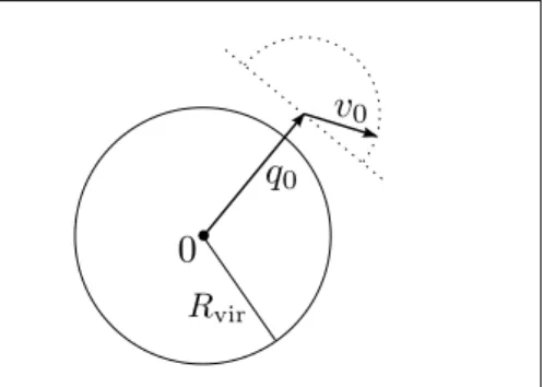
Proposition 2.1.5 Assume the magnetic field B satisfies condition (2.3). Let E > 0 and x

= (q

, v

) ∈ P

with |q

| > R

(E) and hq

, v

i ≥ 0. Then there exists δ > 0 such that

|q

(x

)|

≥ |q

|

+ δt

holds for all t ≥ 0. In particular, the set s

of scattering states is open and satisfies s

= ⁿ x ∈ P | lim

t→∞

|q

(x)| = ∞ ^o .

For s

we obtain the analogous result if we assume hq

, v

i ≤ 0 instead of hq

, v

i ≥ 0.

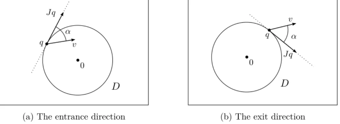
Figure 2.1: Visualization of the scattering condition Proof For |q| ≥ |q

| > R

(E) the inequality |q| · kB(q)k < √

2E holds, so we can define

δ := E −

√ E

√ 2 max

|q|≥|q₀|

|q| · kB(q)k > 0 ,

where the maximum exists due to the convergence |q| · kB(q)k → 0 for |q| → ∞. In particular, we have the estimate

|q| · kB(q)k √

2E ≤ 2E − 2δ (|q| ≥ |q

|) .

We set (q(t), v(t)) := ϕ

(x

) and consider the function f (t) :=

|q(t)|

with derivatives f

(t) = hq(t), v(t)i

and

f

(t) = 2E + hq(t), B(q(t))v(t)i ≥ 2E − |q(t)| · kB (q(t))k √ 2E.

As long as |q(t)| ≥ |q

|, the second derivative satisfies the inequality

f

(t) ≥ 2E − (2E − 2δ) = 2δ. (2.4)

Since f

(0) ≥ 0, this holds for any t ≥ 0 and hence the claim follows.

Remark 2.1.6 The radius R

is the best possible value for this result in the sense that the statement does not hold if one replaces the condition |q

| > R

(E) by |q

| ≥ R

(E).

For the case d = 2 we will see in Chapter 3 that there is a circular orbit of radius r > 0 around the origin if |q|·kB(q)k = √

2E holds for all |q| = r. Hence, if for an energy E > 0 we have |q| · kB(q)k = √

2E for all |q| = R

(E), then an initial value x

= (q

, v

) ∈ P

with |q

| = R

(E) and hq

, v

i = 0 (where v

points into the right direction) yields a circular orbit of radius R

(E). In particular, |q

(x

)| = R

(E) holds for all t ∈ R and therefore, the estimate on the escape rate does not apply. Moreover, x

is not even a

scattering state.

From Proposition 2.1.5 we immediately get the following corollary which says that for sufficiently large energies there are only scattering orbits.

Corollary 2.1.7 For any energy E > E ^f

with E f

:= max

q∈R^d

(|q| · kB(q)k)

2

we have R

(E) = 0 and, in particular, the energy surface P

consists only of scatter- ing states, i.e. P

= s

. Furthermore, as a function of the energy E, R

is strictly decreasing for energies E ≤ E f

.

Since |q

(x

)| ≤ |q

| + |t||v

| as in (1.5), the solution curve can escape to infinity at most at linear speed and Proposition 2.1.5 states that the rate is not less than linear. In fact, for compact sets of scattering states there is a uniform lower bound on the escape speed:

Lemma 2.1.8 Let K ⊆ s

be compact. Then there exist constants C, T > 0 such that

|q

(x)| ≥ Ct holds for all x ∈ K and t ≥ T . The analogous result applies for s

. Proof Let

E

:= min

x∈K

E(x)

denote the minimal energy of initial values in K. There is a time T > 0 and a radius R > 0 such that

|q

(x)| ≥ R > R

(E

) ≥ R

(E(x)) (t ≥ T ) and

hq

(x), v

(x)i ≥ 0

hold for all x ∈ K. From Proposition 2.1.5 we obtain the estimate

|q

(x)|

≥ |q

(x)|

+ δ(E(x))(t − T )

,

where we can choose

δ(E) = E −

√ E

√ 2 max

|q|≥R

|q| · kB(q)k , as the proof showed. Due to

δ

(E) = 1 − 1 2 √

2E max

|q|≥R

|q| · kB(q)k > 1 − 1 2 √

2E

√

2E = 1

2 (E ≥ E

) we have δ(E) ≥ δ(E

) for E ≥ E

and with C := ^p δ(E

) we obtain

|q

(x)|

≥ |q

(x)|

+ C

(t − T )

≥ C

(t − T )

for all x ∈ K and t ≥ T . Hence, the inequality

|q

(x)| ≥ C 2 t

holds for all t ≥ 2T .

In a later section we need to divide by the time t. In order to do this, we have to work around the singularity at t = 0 and therefore introduce the function hti := √

1 + t

for t ∈ R , which can be seen as a smooth modification of the absolute value.

Lemma 2.1.9 The function hti := √

1 + t

for t ∈ R satisfies the following properties:

(i) lim

t→∞

t hti = 1 .

(ii) Given T > 0, there exists a constant C > 0 such that t ≥ Chti holds for t ≥ T.

Proof The first assertion is obvious and the second one holds since

is bounded away

from 0 for t ≥ T > 0.

Using this function, we immediately obtain an analogue for the escape rate in Lemma 2.1.8:

Lemma 2.1.10 Let K ⊆ s

be compact. Then there exist constants C, T > 0 such that

|q

(x)| ≥ Chti holds for all x ∈ K and t ≥ T . Again, the same applies for s

.

2.2 Time decay in a simplified time-dependent magnetic field

Now we turn to the analysis of the asymptotic behaviour of the motion, where we are interested in the limits (2.1) and (2.2), respectively. Before we analyze a time- independent magnetic field in Section 2.3, we start with a simplified version of the motion in a time-dependent magnetic field. In particular, we consider the equation

q ¨ = B(t, q ) ˙ q (2.5)