Magnetic Particle Imaging Signal Based on Theory, Simulation, and
Experiment
by Jan-Philip Gehrcke
A thesis submitted in partial fulfillment of the requirements for the degree
Master of Science with Honors in Physics
supervised by
Prof. Dr. Peter M. Jakob and Dr. Volker C. Behr University of Würzburg, Experimental Physics 5
2010
Magnetic Particle Imaging (MPI) is a novel imaging modality allowing for the detection of the spatial distribution of magnetic nanoparticles at high spatio-temporal resolution. This thesis provides a comprehensive theoretical part, describing the origin and the properties of the signal in MPI as well as the most important dependencies.
The impact of magnetic particle interaction on the MPI signal is investigated by simulation and experiment: it is shown that higher har- monic amplitudesAnare not linearly related to particle concentration c, as misleadingly suggested by LANGEVIN’s single particle model (SPM). Therefore, current linear image reconstruction schemes have to be revised. A more sophisticated magnetization theory matches experimentally gainedAn(c)data very well and consequently is the preferable choice over the SPM.
Finally, this thesis presents a new method for the detection of mag- netic particle agglomerates/clusters based on the nonlinearAn(c)re- lation. This method can be applied to test for specific substances or processes on a molecular level.
1 Introduction 1
2 MPI basics 3
2.1 Overview . . . 3
2.2 Paramagnetism . . . 4
2.3 Superparamagnetism . . . 6
2.4 Ferrofluids . . . 11
2.5 Magnetic Particle Spectroscopy . . . 15
2.6 Magnetic Particle Imaging . . . 30
3 Theory of particle interaction and polydispersity 39 3.1 Polydispersity of magnetic particles . . . 40
3.2 Magnetic particle coupling in dense ferrofluids . . . 45
4 Signal characterization by simulation 51 4.1 Simulation methods . . . 51
4.2 Magnetic Particle Spectroscopy . . . 58
4.3 Magnetic Particle Imaging . . . 68
5 Signal characterization by experiment 75 5.1 MPS concentration dependency . . . 75
5.2 Comparison with simulation . . . 78
6 Application: molecular detection of a substance/process 81 6.1 Classification . . . 81
6.2 Details . . . 83
7 Conclusion 87
Bibliography 89
Appendices 97
Introduction
In 2005, Magnetic Particle Imaging (MPI) has been introduced as an imaging technique to perform background-free detection of the spa- tial distribution of magnetic nanoparticles (made of e.g. iron oxide) in biological tissue [1]. In particular, regarding cellular and molecular imaging or e.g. angiography, MPI may surpass contrast agent-based Magnetic Resonance Imaging (MRI), due to the intrinsic features of the method: high sensitivityand – concurrently –high temporal resolu- tion. Therefore, MPI is a research and diagnostic platform with high potential.
In MPI, the detection of magnetic nanoparticles is based on their non-linear magnetization response. Due to the design of the method,
Figure 1.1:Picture taken out of [2]. Three-dimensional MPI angiography of a mouse, after injecting a magnetic tracer into its tail vein.Color: MPI image, taken out of a time series of three-dimensional datasets. The tracer bolus just goes throughvena cava.Gray: Corresponding anatomy image of the same mouse, done in a separate MRI.
these particles are detected with positive contrast. In a biological system, everything surrounding the particles has a linear magnetization response, ideally leading to no false-positive MPI background signal in medical applications. This is a huge advantage over MRI. Here, magnetic nanoparticles destroy signal, leading to anegative contrast.
Therefore, MPI has the potential to be more conclusive than contrast agent-based MRI.
The first serious MPI results have been presented in 2009 [2]: the authors managed to accomplish a three-dimensional real-time angiogra- phy of a mouse, as indicated in Figure1.1. However, the theory MPI is built on still is in the process of establishment and has to be investigated.
This is where this thesis starts.
Based on important physical concepts like superparamagnetism, magnetic particle spectroscopy and non-linear response in general, the investigations in this work concentrate on the impact of particle concentrationcon the MPI signal. This is very important, since for tomography, the spatial particle distributionc(~x)has to be reconstructed from the MPI signal. To gain a quantitatively correct image, the depen- dency of the MPI signal onchas to be known exactly and accounted for. At this point, previous works used a very simple magnetization the- ory, LANGEVIN’s single particle model, which yields a linear relation between signal anc.
However, due to magnetic dipole-dipole interaction, this actually is a non-linear relation. In this work, the concept of MPI is extended by investigating the impact of magnetic particle interaction theoretically, by simulation, and by experiment.
MPI basics
This chapter is a detailed composition of MPI’s fundamental theory.
The primary goal is to prepare the special approaches and deliberations of this thesis. Another intention of this chapter is to form anentireMPI starter reference, providing theoretical background for all important concepts MPI is constituted of.
2.1 Overview
Aferrofluidis a suspension of magnetic nanoparticles1. If each particle features agiant magnetic moment, the fluid behavessuperparamagnetic, resulting in a strong magnetization response to externally applied mag- netic fields. This phenomenon of superparamagnetism will be described in part2.3.
The interaction of a ferrofluid with an external magnetic field – and, in particular, its magnetization response to it – is the essence of most applications incorporating ferrofluids. Likewise, MPI is built on top of this magnetization response. Fundamental research in MPI starts with the understanding of and the ability to predict a ferrofluid’s magneti- zation behavior. Therefore, after a general description of ferrofluids in part2.4, the simplest case to consider theoretically, a dilute2ferrofluid,
1Particles with dimensions on nanometer scale.
2A ferrofluid with very low particle concentration.
will be discussed in part2.4.3, introducing LANGEVIN’ssingle particle model.
With this theoretical background, the reader is well-prepared to get confronted with “zero-dimensional MPI”: the spectroscopical eval- uation of a ferrofluid’s non-linear magnetization response, which is described in part2.5.
Finally, GLEICHand WEIZENECKER’s methods for determining the spatial distribution of magnetic particles are explained in part2.6.
2.2 Paramagnetism
A system of noninteracting atomic magnetic moments obeys the laws of ideal CURIEparamagnetism [3]. Such a system’s relative magnetization in an external magnetic field is derived now, using a mixture of quantum mechanics and classical statistics.
Consider a single magnetic momentm~ with quantum mechanical behavior1:
~
m=gµB
J~
~, (2.1)
whereg is the LANDÉfactor,µBis BOHR’s magneton,~is the reduced PLANCK constant, and J~ is the total quantum mechanical angular momentum (the sum of spin and orbital contributions). LetJ be the corresponding total angular momentum quantum number.
Consider a z-direction, defined by an external magnetic field B~ (|B|~ =Bz ≡B). The projection ofJ~on thez-axis isJ~z; its absolute value isJz and the corresponding quantum number isjz:
Jz =~jz (2.2)
A quantum mechanical system with total angular momentum number J has exactly2J + 1discrete states, distinguished byjz =−J,−J + 1, . . . , J−1, J. The quantizedJzis leading to a quantizedz-component of the magnetic momentmz:
mz(jz) =gµBJz
~ =gµBjz (2.3)
1E.g. a single atom.
The magnetic moment’s absolute potential energy ismz(jz)·B, so the system’s energy splits up into discrete levels for B 6= 0(ZEEMANN
splitting).
Having these energetically discrete system states, the mean mag- netic momenthmziin field direction for a given temperatureT is easy to derive from classical BOLTZMANNstatistics1:
hmzi=gµBhjzi= gµB Z
jz=+J
X
jz=−J
jze−mz(jz)BkT (2.4) with the partition function
Z =
jz=+J
X
jz=−J
e−mz(jz)BkT . (2.5)
and the BOLTZMANNconstantk.
Considerable manipulation of Equation (2.4) leads to the quantum mechanical BRILLOUINfunctionBJ(B, T), giving a directly evaluat- able expression forhmzi[4]:
hmzi=gµBJBJ(B, T) (2.6) with
BJ(B, T) = 2J + 1 2J coth
2J+ 1 2J a
− 1 2J coth
a 2J
, (2.7) whereas
a = gµBJ B
kT . (2.8)
Paramagnetic system’s magnetization behavior
Now consider a system made of many noninteracting quantum mechan- ical magnetic moments.BJ(B, T)provides the whole system’s relative magnetizationMrel:
Mrel = hMzi M∞
=BJ(B, T). (2.9)
1Here, minimization of magnetic energy is the opponent of thermal agitation.
hMzi is the mean total magnetization in field direction. M∞ is the theoretical saturation magnetization forB → ∞. Saturation is reached, if all magnetic moments had maximum allowed1 alignment with the external magnetic field.
In the absence of an applied field, the independent atomic moments – driven by thermal energy – point at random directions and cancel out each other. Thus, in this case, the system’s total magnetization is zero.
This is characteristic for paramagnetic systems.
2.3 Superparamagnetism
Magnetostatic energy in a ferro- or ferrimagnet is minimized by form- ing the material into magnetic domains. But formation of domains costs energy itself and so there is a critical minimum domain size that mini- mizes the total energy of the system. Consequently, a single particle of a size below the minimal domain size is a homogeneously magnetized single-domain particle [5].
2.3.1 Classical limit: giant magnetic moments
A single-domain particle may consist of104 or even many more single atoms [4]. Below the CURIE temperature, this means that all these atomic magnetic moments in this single magnetic domain are strongly coupled and yield a giant total magnetic moment [5]. The critical particle size, up to which the single-domain state is the energetically preferred one, depends on the actual material and is on the order of1to 100 nm. Detailed numbers regarding different materials are delivered in [6].
The magnetization of a system constituted by noninteracting giant magnetic moments can be perfectly described by the theory of CURIE’s paramagnetism, as introduced in part 2.2. It is just the size of the magnetic moment and the angular momentum quantum numberJ that have to be chosen properly.
When magnetic moment carriers involve so many elementary mag- netic moments as single-domain particles do, quantum effects get ir-
1For quantum mechanical magnetic moments, thez-component is limited as given by Equation2.3. Thus, completely parallel alignment is not allowed.
-20 -10 0 10 20 -1.0
-0.5 0.0 0.5 1.0
Α LHΑL
Figure 2.1: Classical limit of the BRILLOUINfunction, the LANGEVIN
functionL(α). It is used to calculate the relative magnetization of a system of noninteracting and freely rotatable magnetic moments.
relevant. This is due to an extremely high spin quantum number J, allowing virtually free alignment of the giant magnetic moment to an ex- ternally applied field. Then, it is justified to consider the classical limit of CURIE’s paramagnetism, which is represented by the BRILLOUIN
functionBJ(B, T)evaluated forJ → ∞[7] at room temperature:
B∞(B, T) = L
mB kT
(2.10) wherem ≡ |~m|is the giant magnetic moment andL(α)the LANGEVIN
function:
L(α) = coth(α)− 1
α (2.11)
Hence, applying a magnetic field to a system of noninteracting and freely rotatable giant magnetic moments will induce a relative magneti- zation as given byL(α)(see Figure2.1).
2.3.2 Néel and Brown relaxation processes
The classical limit of CURIE’s paramagnetism, when single magnetic moments can be considered as classic magnetic dipoles, is commonly
calledsuperparamagnetism. Particles on the nanometer scale, exhibit- ing giant magnetic moments, are commonly calledsuperparamagnetic particles, with “super” meaning large, as in superconductivity.
But this is not the entire definition of superparamagnetism. Two different relaxation mechanisms have to be distinguished to define it cor- rectly. The consideration of both relaxation types, NÉELand BROWN
relaxation, is very important for applications of superparamagnetic nanoparticles, like MPI.
Néel relaxation
The original meaning of superparamagnetism described a phenomenon pointed out by NÉEL. Consider amechanically fixed single-domain particle. All its elementary quantum mechanical angular momentums are coupled. The resulting giant magnetic moment is rigidly bound by one or more of the possible anisotropies within the crystalline material the particle is made of. It is “frozen” within the particle. For big particles, the anisotropical energy EAI of this bond is very high in comparison with realistic magnetic or thermal energies. But it changes quickly with the particle’s volume. While shrinking this, a critical barrier is passed. Below, the thermal energykT is strong enough to disrupt the magnetic moment’s bonding to the particle itself [5].
The NÉELrelaxation timeτN(EAI/kT)is a gauge for the mobil- ity of a giant magnetic moment within a mechanically fixed particle.
Considerably below the critical particle size, the magnetic moment is free to move and respond to an applied field, resulting inτN to of order 10−9s. Around the critical particle size,τN changes by the factor109 for a volume variation of the factor 2 [8].
Considering a fixed particle with a size below the critical one, an externally applied magnetic field would try to align the giant magnetic moment, fighting againstkT. This is the classical limit of CURIE’s para- magnetism. Hence, the relative magnetization is accurately described by the LANGEVINtheory.
Brown relaxation
In the framework of most applications, magnetic single-domain parti- cles are suspended in a liquid. In these cases, they are able to rotate
mechanically, subjected by BROWNIANmovement. Since the counter- force against such rotation is of hydrodynamic origin, the corresponding BROWNrelaxation timeτB depends on thermal energy, particle volume and the liquid carrier’s viscosity. For water or kerosene as solvent,τB is on the order of10−7s [8].
2.3.3 Critical sizes and characteristical time scales
There are two critical particle volumes. First, Vsd, below which the single-domain state is energetically preferred, exhibiting a giant mag- netic moment. Second, an even smaller volume, Vsp, below which this giant magnetic moment is able to rotate almost freely within the mechanically fixed particle, governed by the NÉELrelaxation timeτN and showing superparamagnetism in its original sense.
Particles with a volume belowVsdbut aboveVsp are important for all applications that require single-domain nanoparticles with huge magnetic moments. But they cannot automatically be considered assu- perparamagnetic(i.e, in the sense of the phenomenon NÉELdiscovered and describable with the LANGEVIN theory). Both of the following conditions must be fulfilled:
• The particles have to be able to rotate mechanically (as is the case when they are solved in a liquid carrier).
• Magnetic field changes and measurements must happen on a larger time scale than given byτB.
Then, it is fundamentally the same as “NÉEL’s superparamagnetism”:
an external field would fight thermal energy and try to align the mag- netic moment by – this time –mechanical rotation of the whole parti- cle. From this it follows that such a system is described correctly by the LANGEVINtheory, too. The case described can be considered as
“BROWN’s superparamagnetism”.
As stated in [5], the critical particle diameter for iron, below which
“real” superparamagnetism in the sense of NÉEL occurs, is 8.5nm.
Below that size, the dominant relaxation mechanism is the NÉELrelax- ation, even for mechanically rotatable particles. This type of relaxation (τN ≈10−9s) is allowing higher excitation and measuring rates than
for bigger particles, which are dominated by mechanical and slower BROWNrelaxation (τB ≈10−7s).
These time scales are important to consider in MPI, e.g. for choosing an appropriate excitation frequency.
2.3.4 Para- vs. superparamagnetism
The fundamental behavior of paramagnetic and superparamagnetic systems is the same, regarding the fact that thermal energy works against the alignment of independent magnetic moments with an applied magnetic field: there is no hysteresis and no residual field. But there are two crucial differences between para- and superparamagnetism:
the field-dependency of the magnetic susceptibilityχandthe absolute magnetization values for the same external field strength.
The magnetic susceptibilityχis defined as the change of magneti- zationM with the magnetic fieldH:
χ= ∂M
∂H, (2.12)
whereH =B/µandµis the magnetic permeability.
While CURIEparamagnetism is stronger than e.g. diagmagnetism, it’s still weak in comparison with magnetically ordered states (like e.g.
ferromagnetism). At room temperature, typical magnetic susceptibili- ties of substances showing CURIE paramagnetism are not higher than 10−2 [3].
Each superparamagnetic particle behaves like a huge atom, with its angular momentum quantum numberJSP being by a factor of several orders of magnitude higher thanJP of a conventional paramagnet. This factor is the same between the resulting magnetic momentsm. The argument of the BRILLOUINand LANGEVINfunction is proportional to the magnetic energy mB. Hence, the factor of several orders of magnitude between JSP and JP arises again for the resulting mag- netic susceptibilities and absolute magnetization values, considering the linear regime of the BRILLOUINand LANGEVINfunctions.
In case of CURIE paramagnetism, it’s actually “impossible” to leave the linear regime: for room temperature, saturation cannot be achieved with the most powerful magnets [4]. Hence, the magnetic
susceptibility χ is field independent: paramagnetic magnetization behavior is always linear.
Superparamagnetic systems can easily be saturated, with moderate magnetic field strengths, generable by conventional magnets. The initial susceptibilityχinit (around zero magnetic field) is much higher than typical magnetic susceptibilities of substances showing CURIE para- magnetism. Here, the discussed factor of several orders of magnitude appears again. χdecreases for bigger field strengths. In the regime of saturation, it converges to zero. Hence,superparamagnetic systems (more general, systems made of giant magnetic moments) can eas- ily be provoked to display non-linear magnetization behavior.
2.4 Ferrofluids
2.4.1 General properties
Ferrofluids (also called ferrocolloids or magnetic fluids) are colloidal fluids, constituted of magnetic particles, which are most often made of or containing ferro- or ferrimagnetic material. The particles are suspended in a carrier fluid, which usually is an organic solvent, like kerosene or water.
Ferrofluids are stabilized with the help of special surfactants the magnetic particle cores are coated with. This prevents local agglomera- tion1due to magnetic andVAN-DER-WAALSforces as well as decom- position of the magnetic cores, leading to highly persistent suspensions.
A true ferrofluid does not settle out and therefore is made of nano- particles [9]. Then, thermal energy is sufficient to overcome gravita- tional effects: BROWNIANmotion keeps the particles homogeneously suspended.
If the particles are noninteracting (far away from each other) and exhibit a giant magnetic moment (like homogeneously magnetized single-domain particles), the whole fluid shows superparamagnetic magnetization behavior and is called asuperparamagnetic ferrofluid.
The liquid carrier allows the particles to rotate mechanically. De- pending on the actual size of the particles within the fluid, either the
1Or “aggregation”: sticking together of particles.
NÉELor the BROWNform of superparamagnetic relaxation is dominat- ing the ferrofluid’s response to externally applied magnetic fields, as explained in part2.3.3.
Particle diameters and magnetic moments
The most widely used ferrofluids are based on spherically shaped na- noparticles, i.e. the cores made of magnetic material are assumed to be spheres. Surface effects lead to spin disordering, so the core is surrounded by a demagnetized layer [10]. The effective magnetic core diameterdonly describes the homogeneously magnetized inner sphere.
This inner part of the particle can be considered as bulk material like in a large-scale solid state. Hence, the bulk saturation magnetizationMsof the corresponding material is valid for the homogeneously magnetized inner sphere, too.
To be able to make a clear statement about the magnetizability of a superparamagnetic ferrofluid, it is essential to know the actual strength of the giant magnetic momentsmthe ferrofluid is constituted of. Since magnetizationM is magnetic momentmper volumeV, the general relation
m=M V (2.13)
can be used to calculate the magnetic moment of a spherically shaped particle in dependence of its magnetic core diameterd:
m(d) = π
6Msd3 (2.14)
During the synthesis of superparamagnetic nanoparticles (different techniques are listed in e.g. [11]), a whole distribution of magnetic core diameters is created. Depending on the actual production method and some size selecting postprocessing (which can be done by filtration and centrifugation), a more or less wide diameter distribution can be found in the resulting ferrofluid.
For an entire description of a particular ferrofluid sample, it is necessary to know the magnetic core diameter probability distribution functionp(d), which can be used to e.g. calculate the mean magnetic momenthm(d)i:
hm(d)i=
Z ∞ 0
p(d)m(d) dd . (2.15)
Measuringp(d)is a non-trivial task, as will be described in part3.1;
but exact awareness is of particular importance: it excludes a huge un- certainty in experiments and enables to reproduce experimental results in simulations.
Ferrofluids with anextremelysharp distributionp(d)are considered as monodisperse, while all other ferrofluids are called polydisperse, i.e. they consist of particles with significantly different magnetic core diameters.
2.4.2 Ferrofluids as contrast agents
In nuclear magnetic resonance imaging (MRI), superparamagnetic nano- particles are well-established as contrast agents for molecular imaging, i.e. gathering both anatomic and information on the molecular level simultaneously: the giant magnetic moments are strong spin-spin re- laxation enhancers and therefore destroy nuclear magnetic resonance signal in their vicinity. In MPI, basically the same contrast agents can be utilized to determine their spatial distribution.
Due to their nontoxicity, superparamagnetic iron-oxide nanopar- ticles (SPIOs) are well-suited for medical applications in organisms like humans [11]. Typically, the iron-oxide particle cores are enveloped in a polysaccharide or synthetic polymer coating. A popular exterior coating material is dextran or citrate, whereas the magnetic core is often made of ferrimagneticmagnetite(Fe3O4) ormaghemite(γFe2O3).
Depending on the actual particle size, shell structure and functionality, there are many SPIO subclasses, like USPIO, MION, VSOP, CLIO and others. A detailed description of these particle classes can be found in [11], [12], and [13]. Furthermore, detailed listings of commercial SPIO agents are shown, including their state of clinical approval.
For medical applications, the coating can be used to ensure bio- compatibility if the core itself is toxic, as is the case for cobalt, which exhibits a much higher magnetic moment per particle volume (bulk saturation magnetizationMs) than e.g. magnetite. Cobalt nanoparticles can be rendered nontoxic, if they are coated with gold [14] or citrate [15].
If noninteracting giant magnetic moments are – as contrast agent – injected into a biological system in form of stable particles,the whole
system can be considered as superparamagnetic ferrofluid, regardless of the particle’s particular realization.
2.4.3 Single Particle Model: dilute ferrofluids’
magnetization theory
The ferrofluid’s magnetization curveM(H)is the key quantity to cal- culate the magnetization response to an externally applied or irradiated magnetic field, if all other parameters are known.
In this part, the magnetization curve of a ferrofluid is discussed in terms of LANGEVIN’s theory of superparamagnetism, i.e. noninteract- ing giant magnetic moments are assumed, as it is well-established in MPI literature, e.g. in [16]. This ferrofluid magnetization model will henceforth referred to asSingleParticleModel (SPM).
Consider a polydisperse ferrofluid constituted of particles yielding an effective magnetic material densityρ∈]0,1], whereas the maximum densityρ= 1corresponds to the bulk material. The goal is to calculate the system’s total magnetizationMSP M(H, ρ)in terms of the SPM, consulting the Equations 2.10 and 2.11, which describe the relative magnetization of a superparamagnetic system. Using the magnetic core diameter probability distribution functionp(d)for averaging, this results in the relative magnetization
Mrel,SP M(H) =
*
L µ0m(d)H kT
!+
. (2.16)
µ0 is the vacuum permeability and kT the thermal energy. With a specific system’s saturation magnetizationM∞(forH → ∞), the total magnetization is generally given by
M(H) =M∞Mrel(H) (2.17) (cf. Equation2.9). Consideringρas theglobaldensity, defining the magnetic phase volume fraction of the sample’s total volume, yields M∞ =ρMs, withMs being the bulk saturation magnetization of the magnetic material. Hence, the SPM’s total magnetization can be ex- pressed as
MSP M(H, ρ) =ρMs
*
L µ0m(d)H kT
!+
. (2.18)
Strictly seen, the SPM is valid only in the limit ρ → 0, because LANGEVIN’s theory of superparamagnetism assumesnoninteracting magnetic moments, which requires infinite distances between them. In reality, the SPM predicts proper ferrofluid magnetization values if the single giant magnetic momentsalmostdo not "see each other". This is the case for verydilutefluids, when the interparticle magnetic coupling energy (due to dipole-dipole exchange interaction) is very small in comparison with the energy of a single moment in the externally applied field.
Neglecting interparticle interactions results in a model that is linear inρ(Equation2.18yieldsMSP M(H, ρ)∝ρ). Obtaining a theoretical model that is valid for moderate and high particle densities, requires the incorporation of magnetic interparticle coupling, which then leads to a non-linear magnetization dependency onρ, as will be discussed in part3.2.
2.5 Magnetic Particle Spectroscopy
Consider a system containing magnetic particles, getting excited by a harmonically oscillating magnetic field. The system then sends out another magnetic field; its magnetization response. If the system’s magnetic susceptibilityχisnotconstant within the range of the excita- tion field strength, the magnetization is non-linearly dependent on the externally applied field strength. As explained in part2.3.4, for systems made of giant magnetic moments,χalready varies for relatively small excitation field strengths.
In case of varyingχ, the considered magnetic system featuresnon- linear response, a phenomenon that is generally known from various physical systems exhibiting non-linear effects. A non-linear magnetiza- tion response contains integer multiples of the harmonically irradiated magnetic field’s frequency, so-called higher harmonics. The higher harmonics’ general origin will be explained mathematically in part 2.5.1, introducing non-linear response theory. Higher harmonics in a ferrofluid’s magnetization response will be analyzed separately in part 2.5.2.
A ferrofluid’s magnetization response can be detected inductively and evaluated spectroscopically. Such an experiment could be con-
sidered as “zero-dimensional MPI”, but a more appropriate term may be Magnetic ParticleSpectroscopy (MPS). MPS can be used to e.g.
investigate the characteristics of MPI contrast agents or for fundamental research regarding the magnetization behavior of ferrofluids.
2.5.1 Nonlinear response theory
Many simple physical systems behave linear. There, e.g. displacements or accelerations are linear to forces and currents are linearly related to voltages, etc. Consider a system with an output quantityf that is the responseto some inputx.f(x)is the transfer function between input and output, characterizing the response behavior of the system.
Linear systems satisfy
flin(x) = K·x+C, (2.19) whereKandCare constants. But, there also are many physical systems obeying non-linear laws due tonon-linear effects, which are of practical importance in various fields of physics. The following example should help to understand a crucial consequence of non-linear response: the generation of higher harmonicsby a harmonically excited non-linear responding system.
Harmonical excitation of a third-order non-linear system Consider a non-linear distortion of a linear system1, which is a third- order distortion in this case:
fnonlin(x) = K·(x+x3) (2.20)
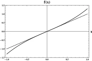
defines the distortion’s relative strength. fnonlin(x)is compared to flin(x)in Figure2.2. Now suppose aharmonicallyoscillating excitation of the system, i.e. the input exactly follows a sine or cosine curve over the timet:
xharmonic(t) = A0+Asin(ωt+φ) (2.21)
1To simplify matters, the offsetCof Equation2.19is set to0.
-1.0 -0.5 0.0 0.5 1.0 -1.5
-1.0 -0.5 0.0 0.5 1.0 1.5
x fHxL
Figure 2.2:A physical system’s transfer functionf(x): response/outputf in dependence of the excitation/inputx. Solid line: predominantly linear responding system with small third-order non-linearity (Equation2.20with = 0.3, K = 1). Dashed line: linear responding system (K = 1).
At this point, the simplest harmonic trajectory is treated, withA0 = 0, A= 1,φ= 0and the excitation frequencyω=ω0:
x(t) = sin(ω0t) (2.22) The response then is
fnonlin(t) = K·sin(ω0t) +sin3(ω0t). (2.23) Using
sin3(y) = 1
4(3 sin(y)−sin(3y)) (2.24) to replacesin3(ω0t)with power-free harmonical terms yields
fnonlin(t) =
K+ 3K 4
sin(ω0t)− K
4 sin(3ω0t). (2.25) The response of a system with linear transfer function would have been flin(t) = K·sin(ω0t), (2.26)
-4 -2 0 2 4 -1.5
-1.0 -0.5 0.0 0.5 1.0 1.5
t fHxHtLL
Figure 2.3: Harmonically excited system’s responsef(x(t)). Solid line:
predominantly linear responding system with third-order non-linearity (Equations 2.22and 2.23 with = 0.3, K = 1, ω0 = 1). Dashed line:
linear responding system (K = 1).
i.e. harmonically oscillating with the excitation frequencyω0 and al- tered amplitude. In contrast, the third-order non-linearity in the transfer function has caused significant changes in the system’s response. As it is obvious from Equation 2.25, the amplitude of the fundamental (excitation) part changes, too and – in particular –a harmonic contribu- tion with frequency3ω0 appears(proportional to). This is a so-called higher harmonicof the fundamental frequencyω0 and since it is the triple fold, it is thethird harmonic. In Figure2.3both, the linear and non-linear systems’ responses to harmonical excitation are compared.
As a result of non-linear response, the overall response signal is distorted: it has contributions ofdifferent frequenciesand, hence, it is no more harmonic.
Generation of higher harmonics: a general consideration An arbitrarily shaped periodic function or signal with periodicityT = 2π/ω0 is a linear combination of thefundamental harmonicpart with frequencyω0 and – depending on the actual signal shape – a number of higher harmonic contributions, whose frequencies are integer multiples ofω0. Contributions with other frequencies will not be found, no matter
what the actual signal’s shape is. This is plausible, since any frequency contributionωthat does not fulfillω =nω0withn∈Zhas no mutual periodicity with2π/ω0. Hence, something else thannω0-contributions would destroy the signal’s overallT-periodicity, implying the fact that any arbitrarily shaped periodic signal must be constituted of single harmonic contributions fulfillingω =nω0.
This was the intuitive and vivid version of a coherence, that, of course, can also be described more entirely and formally: a periodic functionp(t)with the fundamental frequencyω0 = 2π/T can be repre- sented as a FOURIERseries:
p(t) =p(t+T)
=
∞
X
n=0
ancos(nω0t) +bnsin(nω0t) (2.27)
=
∞
X
n=−∞
cneinω0t (2.28)
Hence,p(t)is a linear combination of only harmonical functions (sine, cosine) with different frequenciesnω0 (n∈Z) and distinct amplitudes (an, bn ∈ R). In the course of a FOURIER analysis, the periodic signalp(t)is decomposed in its harmonical constituents, yielding the amplitudes an and bn or cn ∈ C. These coefficients can be used to calculate the power spectral density P(ω)(also simply called the spectrum) of the periodic signalp(t). As argued, this ideally is a discrete spectrum withP(ω)6= 0only forω =nω0.
Think of a system with anarbitrarilyshaped transfer functionf(x), driven/excited periodically by anarbitrarilyshaped input x(t), with only one, but very important, constraint:x(t)must featureT-periodicity.
Independent of the actual forms off(x)andx(t), the responsef(x(t)) then isT-periodic, too:
f(x(t)) =f(x(t+T)) (2.29) In this particular case, Equation2.27implies thatthe response signal of a periodically driven system isalways onlycomposed of discrete harmonical contributions fulfillingω =nω0, no matter if the exci- tation itself is harmonical or not.
Consideringharmonicalinputx(t)(as given by2.22), it is possible to predict the response’s higher harmonic contributions in dependence
of the actual transfer functionf(x). In the example above, it was shown that a third-order non-linearity leads to a3ω0 contribution. Calculating with a second-order non-linearity leads to a2ω0 term, due to
sin2(y) = 1
2(1−cos(2y)), (2.30) providing a reason to believe that there is a strict connection. The intention of the next paragraphs is to enlighten this for then-th order non-linearity.
A transfer function’s non-linearity ofn-th power results in asinn(y) term in the response (in case ofx(t) = sin(ω0t)). In order to understand the harmonical contributions introduced by ann-th power non-linearity, the decomposition ofsinn(y)into a sum of power-free sines or cosines, as it was done in Equations2.24and2.30forn= 2,3, is helpful. The general decomposition rule forn ∈Zis derived in [17]. The result is presented here; even and oddns must be treated separately:
for oddn:
sinn(y) = (−1)(n−1)/2 2n
n
X
k=0
(−1)k n k
!
sin((n−2k)y) (2.31) for evenn :
sinn(y) = (−1)n/2 2n
n
X
k=0
(−1)k n k
!
cos((n−2k)y) (2.32) 2kalways is an even number. Subtracting an even number from an odd- /even number results in an odd/even number, correspondingly. Hence, the formulas above show that ifn isodd,sinn(ω0t)is decomposable into a linear combination of sines withonly oddmultiples of the fun- damental frequencyω0, up tonω0 (fork = 0). Ifniseven,sinn(ω0t) is decomposable into a sum of cosines withonly evenmultiples of the fundamental frequencyω0. Here, the highest appearing frequency is nω0, too. So the harmonical contributions introduced by ann-th power non-linearity are clarified.
The transfer function’s power series representation exactly tells about the type and strength of the included non-linearities. Then-th power addend in the power series off(x)leads to asinn(y)term in the response, introducing – as shown above – harmonical contributions with
frequencies up tonω0. But, if the power series contains all addends with powers betweenn= 1andn =N, this does not necessarily mean that the response containsallhigher harmonics up toN ω0:sinn(ω0t)brings along harmonical oscillations with the frequencies (n −2k)ω0 (for k = 0. . . n) anddifferent amplitudes and phases. Hence, considering more than one power series addend, very special transfer functions resulting in cancellation of one or more harmonic terms are imaginable.
A much more definite conclusion of the discussion above is that ifall oddorall even power series addends aremissing, there will be no mω0 contribution to the system’s response with m odd or even, correspondingly. This fact is important to consider for odd transfer functions (symmetric with respect to the origin;f(x)=−f(−x)) and even transfer functions (symmetric with respect to the x = 0 axis;
f(x)= f(−x)): an even function’s power series only contains even power terms and an odd function is constituted of only odd power terms.
A harmonic excitation as considered here (A0 = 0) keeps the transfer function’s symmetry with respect to an axis or the origin (the excitation takes place symmetrically around the point of symmetry), leading to a responsef(x(t))with the same symmetry. As argued,this results inonly oddoronly evenhigher harmonics in the response.
2.5.2 Ferrofluid magnetization response
The physical basis of MPI is the magnetization response M(H(t)) of magnetic nanoparticles constituting a ferrofluid. In the picture of non-linear response theory, the input is the magnetic field H (at the ferrofluid’s place), changing over the timet. The ferrofluid’s magneti- zation curveM(H)is the transfer function. While input and output are known,in MPS, the sample’s magnetization curve is the unknown quantity. FOURIER analysis of a sample’s magnetization response to a harmonical excitation gives information about the transfer func- tion’s (i.e.M(H)’s) shape (power series representation), as explained in2.5.1. This information answers or at least helps to answer ques- tions about the existence andtype of magnetic particles in the in-
vestigated sample.1
Transfer function: symmetry, non-linearity and Taylor series For a classical magnetic system like a ferrofluid, it is reasonable that M(H) = −M(−H) must always be true, because this is the one- dimensional representation of a magnetization following the magnetic field direction. Thus,M(H)is always symmetric with respect to the ori- gin. As explained in part2.4.3, the magnetization curve of a ferrofluid constituted of noninteracting particles basically follows the LANGEVIN
function. Acoth(α)−1/αshape of course features this origin sym- metry, because both addends do. As a consequence, the power series expansion consists of only odd-order addends:
L(α) = coth(α)− 1 α
≈ 1 3α− 1
45α3+ 2
945α5 − 1
4725α7 +O(α9) (2.33) Equation2.33is the TAYLORexpansion aroundα = 0. At this point, the first-order contribution and the first non-linear term are in a ratio of 15. An expansion aroundαmax =±1.37225results in a ratio of 4.5, i.e.
here the non-linearity carries more than three times more weight. αmax is the numerical solution of
d3
dα3L(α) = 0, (2.34)
solving the problem
αmax = max
d2 dα2L(α)
!
. (2.35)
Aroundαmax, the LANGEVINfunction has the highest curvature and, hence, exhibits the most non-linearity. This can be exploited by an excitation of the system aroundαmax, leading to strong higher harmonic generation. Incidentally, it should be remarked here, that a power series
1In MPI, this is valid, too, but there it is the goal to obtain the informationlocallyand thelocalmagnetization curve is the big unknown, as will be described later.
-3Π -2Π - Π 0 Π 2Π 3Π -1
1
Α LHΑL
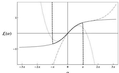
Figure 2.4:Solid line: Langevin functionL(α). Thick dashed line: TAY-
LORseries expansion of 99th order aroundα0 = 0: perfect convergence on the interval]−π, π[, strong divergence beyond. Dashed line: 3rd-order series aroundα0 = 0. Dotdashed line: 3rd-order series aroundα0=π.
expansion around α 6= 0 introduces even-order terms, due to lost symmetry.
Now, the reader may think that a simple calculation with thenth- order TAYLORseries of the magnetization curve enables to predict the higher harmonic contributions up to nω0 in a ferrofluid’s magnetiza- tion response for harmonical input. This is only true for distinct field strength intervals, becauseL(α)isnotanentirefunction: the TAYLOR
series of L(α) is not converging globally due to singularities in the complex plane atmπiwithm=−∞, . . . ,−2,−1,1,2, . . . ,∞.
The TAYLORseries expansion aroundα0 converges toL(α)only for
|α−α0|< r, (2.36) with r being the radius of convergence. r is given by the distance betweenα0and thenearestsingularity toα0in the complex plane. For α0 = 0, the first equally near singularities are at ±iπ. In this case the radius of convergence r is π. For α ∈ R and α /∈ ]−π, π[, the seriesstronglydiverges fromL(α), no matter how many addends are considered. L(α) and its TAYLOR series expansion around α0 = 0
for n = 3 and n = 99 are visualized in Figure2.4. Additionally, a third-order expansion aroundα0 =πis shown.
In MPS, it is possible to keep the magnetic field strength in a distinct interval so thatαstays within an interval of convergence. Then, with thenth-order approximation (series) of the correct magnetization the- ory, it is possible to calculate the higher harmonic amplitudes up to the frequency limitnω0. In MPI, as will be explained soon, quite big field strengths are used to reach the saturation state; in both directions of the magnetization curve. Then, no mutual interval of convergence can be found and a calculation with the power series expansion of the magne- tization curve is senseless, because it does not represent physics any- more. Unfortunately,this circumstance extremely complicates and obstructs an analytical discussion of image reconstruction schemes in MPI.
Excitation: magnetic field irradiation
In MPS, a whole sample is excitedharmonicallyandhomogeneously by an oscillating magnetic field. Since the magnetic field has a di- rection, the most general approach is vector-based. H(t)~ is location- independent in the sample’s volume and generally given by
H(t) =~ H~of f +H~excsin(ω0t). (2.37) H~of f, thestatic offset fieldis of crucial relevance. First of all, an ex- citation with |H~of f| 6= 0 is breaking the symmetry of the response with respect to the origin, resulting in the occurrence of even higher harmonics, besides the odd ones. Furthermore, it can be used to max- imize the generation of higher harmonics, as explained in the part before. As will be explained in part2.6, neat spatial variation of the offset field is used to spatially resolve the magnetization response, leading to the imaging capability in MPI. All this is easy to under- stand forH~of f k H~exc. Then, only|H~of f|and|H~exc|have to be con- sidered, allowing a one-dimensional discussion. In all other cases (H~of f, ~Hexc) 6= zπ (with z ∈ Z), the situation gets more complex and may exhibit exploitable advantages, as will be discussed shortly in part4.3.1, consideringH~of f ⊥H~exc. This topic is also treated in [18].
Response: inductive detection of the MPS signal
After thinking about a vector-based excitation model, a vector-based discussion of the magnetization response is required for integrity. This is conditioned by three decisive points/assumptions:
• The magnetizationM~(t)at the timetis always aligned with the irradiated magnetic field’s directionH(t). This is true, as long as~ the excitation period1/ω0is much bigger than the superparam- agnetic relaxation time (see part2.3.2).
• The absolute value of the magnetization|M~(t)| ≡M depends on the absolute magnetic field strength|H(t)| ≡~ H as given by the magnetization curveM(H).
• Inductive measurement by a coil only detects one magnetization dimension: the projection along the coil’s axis.
This is leading to the general relation
M~(t) = M(|H(t)|)~ · H(t)~
|H(t)|~ , (2.38) with the sample’s magnetization curveM(H). The measurable signal, an induced voltageU(t), is governed by
U(t)∝ d
dtMcoil(t), (2.39)
whereMcoilis the magnetization component aligned with the coil. In the following discussion, Mcoil(t) = M(t)is assumed. U(t)is from now on called the MPS/MPI signal.
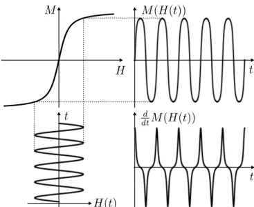
The one-dimensional chain of excitation, transfer function, mag- netization response and its time derivative is visualized in Figure2.5 for|H~of f|= 0. The response’s degree of distortion can be estimated best by means of the time derivative, which is clearly not harmonic anymore (the derivative of a harmonic signal would be harmonic, again).
Everything in the figure was obtained analytically:
U(t)∝ d
dtM(t)∝ d
dtL(Asin(ω0t))
= ω0cot(ω0t)
Asin(ω0t) − Aω0cos(ω0t)
sinh2(Asin(ω0t)), (2.40)
Figure 2.5: Magnetic excitation withHof f = 0(bottom left). Transfer functionM(H)(top left). Magnetization responseM(H(t))(top right).
Response’s time derivative, which is proportional to measurable voltage U(t), which is the MPS signal (bottom right).
withA = 6andω0 = 1.
Fourier analysis of the MPS signal
The next step is to obtain the detected signal’s frequency spectrum, i.e.
resolving the harmonic contributions and their amplitudes. Therefore, the time signal has to be transformed into the frequency domain by a FOURIERtransformationF.
With the analytically gained MPS signal available (Equation2.40), it seems natural to go on analytically to find the exact FOURIER se- ries coefficientsanandbn(Equation2.27) for the first fewn. But the FOURIERseries coefficients’ calculation of Equation2.40can be con- sidered as too difficult or even impossible1, so the analytical discussion stops now.
Instead,U(t)– no matter if it was gained synthetically (analytical- ly/numerically) or in an experiment – is analyzednumericallyusing
1Solving the occurring integrals seemed too hard. This was not discussed further.
adiscreteFOURIERtransformation (DFT). Therefore,U(t)has to be sampled with a specific ratefsample, yielding a set of data pointsUi(ti).
Put simply, the DFT transformsUi(ti)intoAi(ωi), i.e. it resolves the complex amplitude Ai for a specific frequency ωi. Details about pa- rameter selection (which has to be done very carefully), frequency resolution, detection limits and general characteristics of a DFT will be found in the simulation part4.1.1.
Before the DFT result of the synthetically generated MPS signal from Figure2.5is presented, this point is a good opportunity to answer an obvious question:
“We are interested in the frequency spectrum of M(t) to get information about the magnetic properties of the investigated sample. How does the spectrum of M(t) translate into the spectrum of dtdM(t)?”
To answer this question, the time derivative of the complex FOURIER
series representation of a periodic functionA(t)with periodicityT = 2π/ω0is analyzed via Equation2.28:
d
dtA(t) = d dt
∞
X
n=−∞
cneinω0t =
∞
X
n=−∞
cn d dteinω0t
= iω0
∞
X
n=−∞
n·cneinω0t (2.41)
Of course, inductive detection doesnotchange the signal’s fundamen- tal frequency (and, thus, does not produce other frequency contribu- tions). But, the time derivative introduces a factor of iω0n = iω to each FOURIER component. It so to sayamplifiesthe higher harmonic contributions linearly withω. This has an important consequence for numericalsimulations of the MPS/MPI signal: the frequency spectrum of dtdM(t)∝U(t)can be obtained by simply multiplying the frequency spectrum of M(t) with iω. Advantage: time-consuming numerical building of the time derivative is not necessary anymore. Addition- ally, the “iω-method” turns out to be more accurate than the simplest numerical algorithms to build the derivative of a discrete data set.
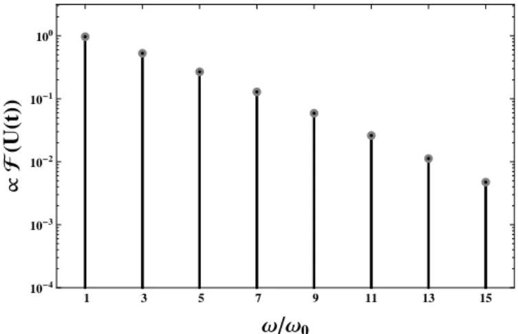
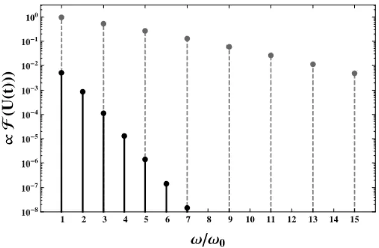
Figure2.6shows the frequency spectrum of the MPS signal corre- sponding to the signal chain in Figure2.5. Both presented methods to gain this spectrum were used:
1 3 5 7 9 11 13 15 10-4
10-3 10-2 10-1 100
ΩΩ0
µFHUHtLL
Figure 2.6:Semilogarithmic diagram of the MPS signal’s FOURIERspec- trumF(U(t)); gained byDFT(absolute values shown). The black bars and dots are the result ofDFT(dtdM(t)); the gray dots are the result of iω·DFT(M(t)).
• sampling and DFT of the analytically gained dtdM(t)
• sampling and DFT ofM(t); multiplication withiωafterward.
As expected, both results equal each other. Furthermore, Figure2.6is a visual proof, attesting the non-linear response theory considerations made above. It shows adiscretespectrum withonly oddharmonics. The highest amplitude can be found in the fundamental contributionω/ω0 = 1; for higher n the amplitudes seem to decay almost exponentially (almost linearly in the semilogarithmic scale).
The MATHEMATICA source code calculating the data shown in Figure2.6can be found in Appendix A.1 (page98).
Evaluation of the MPS signal’s frequency spectrum
The single magnetic moments of a biological system (formed of water, cells and their constituents, big and small proteins, etc.) are several orders of magnitude lowerthan the giant magnetic moments of single- domain particles. As explained in part2.3.4(“para- vs. superparamag- netism”), such a system’s magnetization behavior can be considered as
linear. This assumption is valid1, especially for the low MPI/MPS exci- tation field amplitudesHexc, which typically are on the order of10mT.
Therefore, MPI is often called“background-free”: everythingelse than giant magnetic moments, i.e. magnetic single-domain particles in their function as contrast agentonlycontributes to the fundamental harmonic withω/ω0 = 1. In other words, higher harmonics in the MPS signal’s frequency spectrumprove the existence of contrast agent within the volume of interest. So the prime information extractable from the MPS signal is whether there is contrast agent in the investigated volume or not.
By performing a detailed analysis of the higher harmonic ampli- tudes, it is possible to make much more quantitative and definite state- ments. Consider a ferrofluid magnetization theory thatcorrectlyincor- porates the effect of a whole set of variables like particle concentration, magnetic core diameter (distribution), core material, excitation fre- quency and amplitude (and maybe others) on the transfer function M(H). Then – if all other quantities are known – it is possible to specify the value of an unknown variable from the higher harmonic amplitudes. In a way, MPS is an efficient way to sample the shape of the volume of interest’s magnetization curve with high precision. On the other hand, this means thatMPS in combination with simulations is a promising tool to test a magnetization theory for validity if the whole set of variables is known!
1The reader may have doubts and think of e.g.hemoglobin(the iron-containing oxygen-transport protein in the red blood cells) andferritin(a protein storing and releasing iron in a controlled fashion). Hemoglobin indeed behaves para- or even diamagnetic [19], because it is exhibiting manyspatially separatediron atoms, forming single atomic magnetic moments. Ferritin cores, which can accommodate up to 4500 Fe(III) atoms, have an average magnetic moment of ca. 100µB ≈ O(10−22)Am2 [20], which still is several orders of magnitude lower than the magnetic moment of applied single-domain particles (e.g.10−18Am2for single- domain magnetite cores with16nm diameter). If both are in the investigated volume at the same time, the latter ones simply outstrip the higher harmonic contributions of ferritin by orders of magnitude. Nevertheless, it at least theoretically seems to be possible to use ferritin as contrast agent itself, by exploiting itsextremely low non-linear magnetization behavior.
2.6 Magnetic Particle Imaging
In MPI, it is the goal to measure the spatial distribution of contrast agent in a sample’s volume (volume of interest,VOI), i.e. the contrast agent’s particle densityρat location~x.
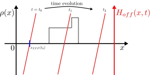
For the step from MPS to MPI, the MPS signal has to be spatially encoded, i.e. it has to be detected and evaluated for a small sub-volume of the VOI. For realizing this, the basic idea is to apply a spatially dependent offset fieldHof f(~x) to the sample: |Hof f|is zero in a so- calledfield-free point(FFP), but raises extremely fast with increasing distance from the FFP, resulting ina strong offset field everywhere, except in the FFP and its near vicinity. By doing this, the contrast agent in the major part of the sample’s volume is magneticallysaturated, which is “switching off” higher harmonics from this VOI’s part, as will be shown in part 2.6.1. If the whole VOI gets excited in this configuration, the emitted signal tells about contrast agent only in the FFP and its near vicinity; the rest of the sample ismasked out.
By moving the FFP – using a temporally dependent offset field Hof f(~x, t)– it is possible to scan the whole VOI [1].ρ(~x), the “image”, can then be obtained by acquiring the emitted signal over the time, fol- lowed by an image reconstruction scheme. The specific reconstruction algorithm depends on the actual signal acquisition method. Two of these methods and their corresponding reconstruction schemes will be introduced in parts2.6.2and2.6.3.
A conceivable extension of the FFP principle is to realize spatial encoding using afield free line(FFL). This implicates averaging and results in a higher signal to noise ratio per overall acquisition time, as pointed out in [21]. The FFL approach will not be discussed further in this thesis.