Aachen
Department of Computer Science
Technical Report
A Dependency Pair Framework for Innermost Complexity Analysis of Term Rewrite Systems
Lars Noschinski, Fabian Emmes, and J¨ urgen Giesl
ISSN 0935–3232 · Aachener Informatik Berichte · AIB-2011-03 RWTH Aachen · Department of Computer Science · April 2011
The publications of the Department of Computer Science of RWTH Aachen Universityare in general accessible through the World Wide Web.
http://aib.informatik.rwth-aachen.de/
A Dependency Pair Framework for Innermost Complexity Analysis of Term Rewrite Systems
⋆Lars Noschinski1, Fabian Emmes2, and J¨urgen Giesl2
1 Institut f¨ur Informatik, TU Munich, Germany
2 LuFG Informatik 2, RWTH Aachen University, Germany
Abstract. We present a modular framework to analyze the innermost runtime complexity of term rewrite systems automatically. Our method is based on the dependency pair framework for termination analysis. In contrast to previous work, we developed adirectadaptation of successful termination techniques from the dependency pair framework in order to use them for complexity analysis. By extensive experimental results, we demonstrate the power of our method compared to existing techniques.
1 Introduction
In practice, termination is often not sufficient, but one also has to ensure that algorithms terminate in reasonable (e.g., polynomial) time. While termination of term rewrite systems (TRSs) is well studied, only recently first results were obtained which adapt termination techniques in order to obtain polynomial com- plexity bounds automatically, e.g., [2–5,7,9,15,16,19–21,23,26,27]. Here, [3,15,16]
consider thedependency pair (DP) method [1,10,11,14], which is one of the most popular termination techniques for TRSs.3 Moreover, [27] introduces a related modular approach for complexity analysis based on relative rewriting.
Techniques for automated innermost termination analysis of term rewriting are very powerful and have been successfully used to analyze termination of programs in many different languages (e.g., Java [24],Haskell [12], Prolog[25]).
Hence, by adapting these termination techniques, the ultimate goal is to obtain approaches which can also analyze the complexity of programs automatically.
In this paper, we present a fresh adaptation of the DP framework forinner- most runtime complexity analysis [15]. In contrast to [3, 15, 16], we follow the original DP framework closely. This allows us to directly adapt the several termi- nation techniques (“processors”) of the DP framework for complexity analysis.
Like [27], our method is modular. But in contrast to [27], which allows to inves- tigate derivational complexity [17], we focus on innermost runtime complexity.
Hence, we can inherit the modularity aspects of the DP framework and benefit from its transformation techniques, which increases power significantly.
⋆Supported by the DFG grant GI 274/5-3.
3 There is also a related area of implicit computational complexity which aims at characterizing complexity classes, e.g., using type systems [18], bottom-up logic pro- grams [13], and also using termination techniques like dependency pairs (e.g., [20]).
After introducing preliminaries in Sect. 2, in Sect. 3 we adapt the concept of dependency pairs from termination analysis to so-called dependency tuples for complexity analysis. While theDP framework for termination works onDP problems, we now work onDT problems(Sect. 4). Sect. 5 adapts the “processors”
of the DP framework in order to analyze the complexity of DT problems. We implemented our contributions in the termination analyzerAProVE. Due to the results of this paper,AProVEwas the most powerful tool for innermost runtime complexity analysis in the International Termination Competition 2010. This is confirmed by our experiments in Sect. 6, where we compare our technique empirically with previous approaches. All proofs can be found in the appendix.
2 Runtime Complexity of Term Rewriting
See e.g. [6] for the basics of term rewriting. LetT(Σ,V) be the set of all terms over a signatureΣand a set of variablesV where we just writeT ifΣandV are clear from the context. Thearityof a function symbolf ∈Σis denoted by ar(f) and the size of a term is|x|= 1 forx∈ V and|f(t1, . . . , tn)|= 1+|t1|+. . .+|tn|.
Thederivation height of a termtw.r.t. a relation→is the length of the longest sequence of →-steps starting witht, i.e., dh(t,→) = sup{n| ∃t′ ∈ T, t→nt′}, cf. [17]. Here, for any setM ⊆N∪ {ω}, “supM” is the least upper bound ofM. Thus, dh(t,→) =ωiftstarts an infinite sequence of→-steps.
As an example, consider R={dbl(0)→0, dbl(s(x))→s(s(dbl(x)))}. Then dh(dbl(sn(0)),→R) =n+ 1, but dh(dbln(s(0)),→R) = 2n+n−1.
For a TRS R with defined symbols Σd ={root(ℓ) | ℓ → r ∈ R }, a term f(t1, . . . , tn) is basic iff ∈Σd andt1, . . . , tn do not contain symbols fromΣd. So forRabove, the basic terms aredbl(sn(0)) anddbl(sn(x)) forn∈N,x∈ V. Theinnermost runtime complexity function ircR maps anyn∈Nto the length of the longest sequence of →i R-steps starting with a basic term t with |t| ≤n.
Here, “→i R” is the innermost rewrite relation andTBis the set of all basic terms.
Definition 1 (ircR [15]). For a TRS R, its innermost runtime complexity function ircR:N→N∪{ω} isircR(n) = sup{dh(t,→i R)|t∈ TB,|t| ≤n}.
If one only considers evaluations of basic terms, the (runtime) complexity of thedbl-TRS is linear (ircR(n) =n−1 forn≥2). But if one also permits evalu- ations starting withdbln(s(0)), the complexity of thedbl-TRS is exponential.
When analyzing the complexity ofprograms, one is typically interested in (in- nermost) evaluations where a defined function likedblis applied to data objects (i.e., terms without defined symbols). Therefore,(innermost) runtime complexi- ty corresponds to the usual notion of “complexity” for programs [4,5]. So for any TRSR, we want to determine the asymptotic complexity of the function ircR. Definition 2 (Asymptotic Complexities). Let C= {Pol0,Pol1,Pol2, ...,?}
with the order Pol0<Pol1<Pol2<. . .<?. Let⊑be the reflexive closure of<. For any function f :N→N∪ {ω}we define its complexity ι(f)∈Cas follows:
ι(f) =Polk if kis the smallest number with f(n)∈ O(nk)andι(f) = ? if there is no such k. For any TRS R, we define its complexity ιR asι(ircR).
So thedbl-TRSRhas linear complexity, i.e.,ιR=Pol1. As another example, consider the following TRS Rwhere “m” stands for “minus”.
Example 3. m(x, y)→if(gt(x, y), x, y) gt(0, k)→false p(0)→0 if(true, x, y)→s(m(p(x), y)) gt(s(n),0)→true p(s(n))→n if(false, x, y)→0 gt(s(n),s(k))→gt(n, k)
Here, ιR=Pol2 (e.g.,m(sn(0),sk(0))starts evaluations of quadratic length).
3 Dependency Tuples
In the DP method, for everyf ∈Σd one introduces a fresh symbolf♯with ar(f)
= ar(f♯). For a termt=f(t1, . . . , tn) withf ∈Σd we define t♯=f♯(t1, . . . , tn) and letT♯={t♯|t∈ T,root(t)∈Σd}. LetPos(t) contain all positions oftand letPosd(t) ={π|π∈ Pos(t),root(t|π)∈Σd}. Then for every ruleℓ→rwith Posd(r) ={π1, . . . , πn}, itsdependency pairs areℓ♯→r|♯π1, . . . ,ℓ♯→r|♯πn.
While DPs are used for termination, for complexity we have to regard all defined functions in a right-hand side at once. Thus, we extend the concept of weak dependency pairs [15, 16] and only build a singledependency tuple ℓ→ [r|♯π1, . . . , r|♯πn] for eachℓ→r. To avoid handling tuples, for everyn≥0, we intro- duce a freshcompound symbolComnof aritynand useℓ♯→Comn(r|♯π1,..., r|♯πn).
Definition 4 (Dependency Tuple).Adependency tupleis a rule of the form s♯→Comn(t♯1, . . . , t♯n)fors♯, t♯1, . . . , t♯n ∈ T♯. Letℓ→rbe a rule withPosd(r) = {π1, . . . , πn}. Then DT(ℓ→r)is defined4 to beℓ♯→Comn(r|♯π1, . . . , r|♯πn). For a TRS R, letDT(R) ={DT(ℓ→r)|ℓ→r∈ R}.
Example 5. For the TRSRfrom Ex. 3,DT(R)is the following set of rules.
m♯(x, y)→Com2(if♯(gt(x, y), x, y),gt♯(x, y)) (1) if♯(true, x, y)→Com2(m♯(p(x), y),p♯(x)) (2)
if♯(false, x, y)→Com0 (3)
p♯(0)→Com0 (4) p♯(s(n))→Com0 (5) gt♯(0, k)→Com0 (6) gt♯(s(n),0)→Com0 (7) gt♯(s(n),s(k))→Com1(gt♯(n, k)) (8) For termination, one analyzeschains of DPs, which correspond to sequences of function calls that can occur in reductions. Since DTs representseveral DPs, we now obtainchain trees. (This is analogous to thepath detection in [16]).
Definition 6 (Chain Tree). Let D be a set of DTs and Rbe a TRS. Let T be a (possibly infinite) tree whose nodes are labeled with both a DT from Dand a substitution. Let the root node be labeled with (s♯→Comn(. . .)|σ). ThenT is a (D,R)-chain tree fors♯σ if the following holds for all nodes ofT: If a node is labeled with (u♯→Comm(v1♯, . . . , vm♯ )|µ), thenu♯µ is in normal form w.r.t.
R. Moreover, if this node has the children (p♯1 → Comm1(. . .)| τ1), . . . ,(p♯k → Comm
k(. . .)|τk), then there are pairwise different i1, . . . , ik ∈ {1, . . . , m} with
4 To makeDT(ℓ→r) unique, we use a total order<on positions whereπ1< ... < πn.
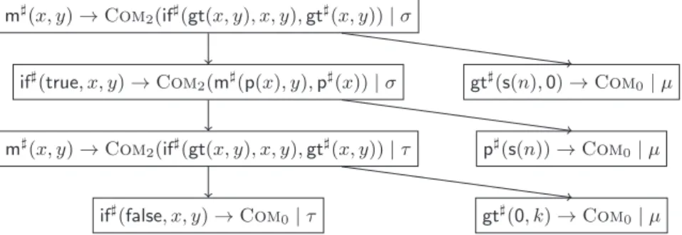
m♯(x, y)→Com2(if♯(gt(x, y), x, y),gt♯(x, y))|σ
if♯(true, x, y)→Com2(m♯(p(x), y),p♯(x))|σ gt♯(s(n),0)→Com0|µ
m♯(x, y)→Com2(if♯(gt(x, y), x, y),gt♯(x, y))|τ p♯(s(n))→Com0|µ
if♯(false, x, y)→Com0|τ gt♯(0, k)→Com0|µ
Fig. 1.Chain Tree for the TRS from Ex. 3
v♯ijµ→i ∗Rp♯jτj for all j∈ {1, . . . , k}. A path in the chain tree is called a chain.5 Example 7. For the TRSRfrom Ex. 3 and its DTs from Ex. 5, the tree in Fig.
1 is a (DT(R),R)-chain tree for m♯(s(0),0). Here, we use substitutions with σ(x) =s(0)andσ(y) =0,τ(x) =τ(y) =0, andµ(n) =µ(k) =0.
For any term s♯ ∈ T♯, we define its complexity as the maximal number of nodes in any chain tree fors♯. However, sometimes we do not want to countall DTs in the chain tree, but only the DTs from some subsetS. This will be crucial to adapt termination techniques for complexity, cf. Sect. 5.2 and 5.4.
Definition 8 (Complexity of Terms, CplxhD,S,Ri). LetD be a set of depen- dency tuples, S ⊆ D,Ra TRS, and s♯∈ T♯. Then CplxhD,S,Ri(s♯)∈N∪ {ω}is the maximal number of nodes from S occurring in any (D,R)-chain tree fors♯. If there is no (D,R)-chain tree fors♯, thenCplxhD,S,Ri(s♯) = 0.
Example 9. For R from Ex. 3, we have CplxhDT(R),DT(R),Ri(m♯(s(0),0)) = 7, since the maximal tree for m♯(s(0),0)in Fig. 1 has 7 nodes. In contrast, if S is DT(R)without the gt♯-DTs(6)– (8), thenCplxhDT(R),S,Ri(m♯(s(0),0)) = 5.
Thm. 10 shows how dependency tuples can be used to approximate the derivation heights of terms. More precisely, CplxhDT(R),DT(R),Ri(t♯) is an up- per bound fort’s derivation height, provided thattis inargument normal form.
Theorem 10 (Cplx bounds Derivation Height). Let R be a TRS. Let t= f(t1, . . . , tn) ∈ T be in argument normal form, i.e., all ti are normal forms w.r.t.R. Then we havedh(t,→i R)≤ CplxhDT(R),DT(R),Ri(t♯). IfRis confluent, we have dh(t,→i R) =CplxhDT(R),DT(R),Ri(t♯).
Note that DTs are much closer to the original DP method than the weak DPsof [15,16]. While weak DPs also use compound symbols, they only consider thetopmost defined function symbols in right-hand sides of rules. Hence, [15,16]
does not use DP concepts when defined functions occur nested on right-hand
5 Thesechainscorrespond to the “innermost chains” in the DP framework [1, 10, 11].
To handlefull (i.e., not necessarily innermost) runtime complexity, one would have to adapt Def. 6 (e.g., thenu♯µwould not have to be in normal form).
sides (as in them- and the firstif-rule) and thus, it cannot fully benefit from the advantages of the DP technique. Instead, [15, 16] has to impose several restric- tions which are not needed in our approach, cf. Footnote 10. The close analogy of our approach to the DP method allows us to adapt the termination tech- niques of the DP framework in order to work on DTs (i.e., in order to analyze CplxhDT(R),DT(R),Ri(t♯) for all basic terms t of a certain size). Using Thm. 10, this yields an upper bound for the complexity ιR of the TRS R, cf. Thm. 14.
Note that there exist non-confluent TRSs6 whereCplxhDT(R),DT(R),Ri(t♯) is ex- ponentially larger than dh(t,→i R) (in contrast to [15, 16], where the step from TRSs to weak DPs does not change the complexity). However, our main interest is in TRSs corresponding to “typical” (confluent)programs. Here, the step from TRSs to DTs does not “lose” anything (i.e., one has equality in Thm. 10).
4 DT Problems
Our goal is to find out automatically how largeCplxhD,S,Ri(t♯) could be for basic termstof size n. To this end, we will repeatedly replace the triplehD,S,Riby
“simpler” triples hD′,S′,R′iand examineCplxhD′,S′,R′i(t♯) instead.
This is similar to the DP framework where termination problems are repre- sented by so-called DP problems (consisting of a set of DPs and a set of rules) and where DP problems are transformed into “simpler” DP problems repeatedly.
For complexity analysis, we consider “DT problems” instead of “DP problems”
(our “DT problems” are similar to the “complexity problems” of [27]).
Definition 11 (DT Problem).LetRbe a TRS,Da set of DTs,S ⊆ D. Then hD,S,Riis a DT problemandR’scanonical DT problemishDT(R),DT(R),Ri.
Thm. 10 showed the connection between the derivation height of a term and the maximal number of nodes in a chain tree. This leads to the definition of the complexity of a DT problemhD,S,Ri. It is defined as the asymptotic complexity of the function irchD,S,Ri which maps any numbernto the maximal number of S-nodes in any (D,R)-chain tree fort♯, wheretis a basic term of at most sizen.
Definition 12 (Complexity of DT Problems).For a DT problemhD,S,Ri, its complexity functionisirchD,S,Ri(n) = sup{ CplxhD,S,Ri(t♯)|t∈ TB,|t| ≤n}.
We define the complexityιhD,S,Ri of the DT problem as ι(irchD,S,Ri).
Example 13. Consider Rfrom Ex. 3 and let D=DT(R) ={(1), . . . ,(8)}. For t∈ TB with |t|=n, the maximal chain tree fort♯ has approximatelyn2 nodes, i.e., irchD,D,Ri(n)∈ O(n2). Thus,hD,D,Ri’s complexity isιhD,D,Ri=Pol2.
Thm. 14 shows that to analyze the complexity of a TRSR, it suffices to ana- lyze the complexity of its canonical DT problem: By Def. 2,ιRis the complexity of the runtime complexity function ircRwhich mapsnto the length of the longest innermost rewrite sequence starting with a basic term of at most sizen. By Thm.
10, this length is less than or equal to the sizeCplxhDT(R),DT(R),Ri(t♯) of the max-
6 Consider the TRSf(s(x))→f(g(x)),g(x)→x,g(x)→a(f(x)). Its runtime complex- ity is linear, but for anyn >0, we haveCplxhDT(R),DT(R),Ri(f♯(sn(0))) = 2n+1−2.
imal chain tree for any basic termtof at most sizen, i.e., to irchDT(R),DT(R),Ri(n).
Theorem 14 (Upper bound for TRSs via Canonical DT Problems).
Let Rbe a TRS and let hD,D,Ri be the corresponding canonical DT problem.
Then we have ιR⊑ιhD,D,Ri and ifRis confluent, we have ιR=ιhD,D,Ri. Now we can introduce our notion of processors which is analogous to the “DP processors” for termination [10, 11] (and related to the “complexity problem processors” in [27]). A DT processor transforms a DT problem P to a pair (c, P′) of an asymptotic complexity c∈C and a DT problemP′, such thatP’s complexity is bounded by the maximum of cand of the complexity ofP′. Definition 15 (Processor,⊕).ADT processorProcis a functionProc(P)
= (c, P′) mapping any DT problemP to a complexity c∈Cand a DT problem P′. A processor is sound ifιP ⊑c⊕ιP′. Here, “⊕” is the “maximum” function onC, i.e., for anyc, d∈C, we definec⊕d=difc⊑dandc⊕d=c otherwise.
To analyze the complexityιR of a TRS R, we start with the canonical DT problem P0 = hDT(R), DT(R),Ri. Then we apply a sound processor to P0
which yields a result (c1, P1). Afterwards, we apply another (possibly different) sound processor toP1which yields (c2, P2), etc. This is repeated until we obtain a solved DT problem (whose complexity is obviouslyPol0).
Definition 16 (Proof Chain, Solved DT Problem). We call a DT problem P =hD,S,Ri solved, if S=∅. A proof chain7 is a finite sequenceP0 c1
;P1 c2
; . . .;ck Pk ending with a solved DT problem Pk, such that for all0≤i < k there exists a sound processor Proci with Proci(Pi) = (ci+1, Pi+1).
By Def. 15 and 16, for everyPi in a proof chain,ci+1⊕. . .⊕ck is an upper bound for its complexityιPi. Here, the empty sum (fori=k) is defined asPol0. Theorem 17 (Approximating Complexity by Proof Chain). Let P0 c1
; P1 c2
;. . .;ck Pk be a proof chain. ThenιP0⊑c1⊕. . .⊕ck.
Thm. 14 and 17 now imply that our approach for complexity analysis is correct.
Corollary 18 (Correctness of Approach).IfP0is the canonical DT problem for a TRS RandP0
c1
;. . .;ck Pk is a proof chain, thenιR⊑c1⊕. . .⊕ck.
5 DT Processors
In this section, we present several processors to simplify DT problems automat- ically. To this end, we adapt processors of the DP framework for termination.
Theusable rules processor (Sect. 5.1) simplifies a problemhD,S,Riby delet- ing rules fromR. Thereduction pair processor(Sect. 5.2) removes DTs fromS, based on term orders. In Sect. 5.3 we introduce thedependency graph, on which theleaf removal andknowledge propagation processor (Sect. 5.4) are based. Fi- nally, Sect. 5.5 adapts processors based on transformations likenarrowing.
7 Of course, one could also define DT processors that transform a DT problemP into a complexity c and a set {P1′, . . . , Pn′} such that ιP ⊑ c⊕ιP′
1 ⊕. . .⊕ιPn′. Then instead of a proof chain one would obtain a proof tree.
5.1 Usable Rules Processor
As in termination analysis, we can restrict ourselves to those rewrite rules that can be used to reduce right-hand sides of DTs (when instantiating their variables with normal forms). This leads to the notion ofusable rules.8
Definition 19 (Usable Rules UR [1]). For a TRS Rand any symbol f, let RlsR(f) ={ℓ→r|root(ℓ) =f}. For any termt,UR(t)is the smallest set with
• UR(x) =∅if x∈ V and
• UR(f(t1, . . . , tn)) =RlsR(f) ∪ S
ℓ→r∈RlsR(f)UR(r)∪S
1≤i≤nUR(ti) For any set Dof DTs, we define UR(D) =S
s→t∈ D UR(t).
So forRandDT(R) in Ex. 3 and 5,UR(DT(R)) contains just thegt- and the p-rules. The following processor removes non-usable rules from DT problems.9 Theorem 20 (Usable Rules Processor). Let hD,S,Ri be a DT problem.
Then the following processor is sound:Proc(hD,S,Ri) = (Pol0,hD,S,UR(D)i).
So when applying the usable rules processor on the canonical DT problem hD,D,RiofRfrom Ex. 3, we obtainhD,D,R1iwhereR1are thegt- andp-rules.
5.2 Reduction Pair Processor
Using orders is one of the most important methods for termination or complexity analysis. In the most basic approach, one tries to find a well-founded order≻such that every reduction step (strictly) decreases w.r.t. ≻. This proves termination and most reduction orders also imply some complexity bound, cf. e.g. [7, 17].
However, direct applications of orders have two main drawbacks: The obtained bounds are often far too high to be useful and there are many TRSs that cannot be oriented strictly with standard orders amenable to automation, cf. [27].
Therefore, thereduction pair processor of the DP framework only requires a strict decrease (w.r.t. ≻) for at least one DP, while for all other DPs and rules, a weak decrease (w.r.t.%) suffices. Then the strictly decreasing DPs can be deleted. Afterwards one can use other orders (or termination techniques) to solve the remaining DP problem. To adapt the reduction pair processor for complexity analysis, we have to restrict ourselves to Com-monotonic orders.10 Definition 21 (Reduction Pair). Areduction pair (%,≻)consists of a stable monotonic quasi-order%and a stable well-founded order≻which are compatible
8 The idea of applying usable rules also for complexity analysis is due to [15], which introduced a technique similar to Thm. 20.
9 While Def. 19 is the most basic definition ofusable rules, the processor of Thm. 20 can also be used with more sophisticated definitions of “usable rules” (e.g., as in [11]).
10In [15] “Com-monotonic” is called “safe”. Note that our reduction pair processor is much closer to the original processor of the DP framework than [15]. In the main theorem of [15], all (weak) DPs have to be oriented strictly in one go. Moreover, one even has to orient the (usable) rules strictly. Finally, one is either restricted to non- duplicating TRSs or one has to use orderings≻that are monotonic onall symbols.
(i.e.,%◦≻◦%⊆ ≻). An order≻isCom-monotoniciffComn(s♯1, ..., s♯i, ..., s♯n)≻ Comn(s♯1, ..., t♯, ..., s♯n) for all n∈ N, all 1 ≤i ≤n, and all s♯1, . . . , s♯n, t♯ ∈ T♯ withs♯i ≻t♯. A reduction pair(%,≻)isCom-monotonic iff≻isCom-monotonic.
For a DT problem (D,S,R), we orientD ∪ Rby%or≻. But in contrast to the processor for termination, if a DT is oriented strictly, we may not remove it fromD,but only fromS. So the DT is not counted anymore for complexity, but it may still be used in reductions.11 We will improve this later in Sect. 5.4.
Example 22. This TRS Rshows why DTs may not be removed fromD.12 f(0)→0 f(s(x))→f(id(x)) id(0)→0 id(s(x))→s(id(x)) LetD=DT(R) ={f♯(0)→Com0, f♯(s(x))→Com2(f♯(id(x)),id♯(x)), id♯(0)→ Com0, id♯(s(x)) →Com1(id♯(x))}, where UR(D) are just the id-rules. For the DT problem hD,S,UR(D)i with S =D, there is a linear polynomial interpre- tation [·] that orients the first two DTs strictly and the remaining DTs and usable rules weakly: [0] = 0,[s](x) =x+ 1,[id](x) =x,[f♯](x) =x+ 1,[id♯](x) = 0,[Com0] = 0,[Com1](x) = x,[Com2](x, y) = x+y. If one would remove the first two DTs from D, there is another linear polynomial interpretation that orients the remaining DTs strictly (e.g., by [id♯](x) =x+ 1). Then, one would falsely conclude that the whole TRS has linear runtime complexity.
Hence, the first two DTs should only be removed fromS, not from D. This results inhD,S′,UR(D)iwhereS′ consists of the last two DTs. These DTs can occur quadratically often in reductions with D ∪ UR(D). Hence, when trying to orient S′ strictly and the remaining DTs and usable rules weakly, we have to use a quadratic polynomial interpretation (e.g., [0] = 0,[s](x) =x+ 2,[id](x) = x,[f♯](x) = x2,[id♯](x) = x+ 1,[Com0] = 0,[Com1](x) = x,[Com2](x, y) = x+y). Hence, now we (correctly) conclude that the TRS has quadratic runtime complexity (indeed, dh(f(sn(0)),→i R) =(n+1)·(n+2)
2 ).
So when applying the reduction pair processor to hD,S,Ri, we obtain (c, hD,S \ D≻,Ri). Here, D≻ are the strictly decreasing DTs from Dand c is an upper bound for the number ofD≻-steps in innermost reductions withD ∪ R.
Theorem 23 (Reduction Pair Processor).LetP =hD,S,Ribe a DT prob- lem and (%,≻) be a Com-monotonic reduction pair. Let D ⊆ %∪ ≻,R ⊆ %, and c ⊒ι(irc≻) for the function irc≻(n) = sup{dh(t♯,≻) | t ∈ TB,|t| ≤n}.13 Then the following processor is sound:Proc(hD,S,Ri) = (c, hD,S \ D≻,Ri).
11This idea is also used in [27]. However, [27] treats derivational complexity instead of (innermost) runtime complexity, and it operates directly on TRSs and not on DPs or DTs. Therefore, [27] has to impose stronger restrictions (it requires≻to be monotonic onallsymbols) and it does not use other DP- resp. DT-based processors.
12An alternative such example is shown in [8, Ex. 11].
13As noted by [22], this can be weakened by replacing dh(t♯,≻) with dh(t♯,≻ ∩→i D/R), where→D/R=→∗R◦ →D◦ →∗Rand→i D/Ris the restriction of→D/Rwhere in each rewrite step with→Ror→D, the arguments of the redex must be in (D ∪ R)-normal form, cf. [3]. Such a weakening is required to use reduction pairs based on path orders where a termt♯may start≻-decreasing sequences of arbitrary (finite) length.
To automate Thm. 23, we need reduction pairs (%,≻) where an upper bound c forι(irc≻) is easy to compute. This holds for reduction pairs based onpolyno- mial interpretations with coefficients fromN(which are well suited for automa- tion). ForCom-monotonicity, we restrict ourselves tocomplexity polynomial in- terpretations (CPIs) [·] where [Comn](x1, ..., xn) =x1+...+xn for all n∈N. This is the “smallest” polynomial which is monotonic inx1, ..., xn. AsComnonly occurs on right-hand sides of inequalities, [Comn] should be as small as possible.
Moreover, aCPI interprets constructorsf ∈Σ\Σdby polynomials [f](x1, ..., xn) =a1x1+. . .+anxn+bwhere b∈Nandai∈ {0,1}. This ensures that the mapping from constructor ground termst∈ T(Σ\Σd,∅) to their interpretations is in O(|t|), cf. [7, 17]. Note that the interpretations in Ex. 22 wereCPIs.
Thm. 24 shows how such interpretations can be used14 for the processor of Thm. 23. Here, as an upper boundcforι(irc≻), one can simply takePolm, where mis the maximal degree of the polynomials in the interpretation.
Theorem 24 (Reduction Pair Processor with Polynomial Interpreta- tions). Let P =hD,S,Ri be a DT problem and let % and≻ be induced by a CPI[·]. Letm∈Nbe the maximal degree of all polynomials [f♯], for allf♯ with f ∈ Σd. Let D ⊆ %∪ ≻ and R ⊆ %. Then the following processor is sound:
Proc(hD,S,Ri) = (Polm, hD,S \ D≻,Ri).
Example 25. This TRS [1] illustrates Thm. 24, whereq(x, y, y)computes⌊xy⌋.
q(0,s(y),s(z))→0 q(s(x),s(y), z)→q(x, y, z) q(x,0,s(z))→s(q(x,s(z),s(z)))
The dependency tuples Dof this TRS are
q♯(0,s(y),s(z))→Com0 (9) q♯(s(x),s(y), z)→Com1(q♯(x, y, z)) (10) q♯(x,0,s(z))→Com1(q♯(x,s(z),s(z))) (11) As the usable rules are empty, Thm. 20 transforms the canonical DT problem to hD,D,∅i. Consider the CPI[0] = 0,[s](x) =x+1,[q♯](x, y, z) =x+1,[Com0] = 0, [Com1](x) = x. With the corresponding reduction pair, the DTs (9) and (10)are strictly decreasing and(11)is weakly decreasing. Moreover, the degree of [q♯] is 1. Hence, the reduction pair processor returns (Pol1,hD,{(11)},∅i).
Unfortunately, no reduction pair based on CPIs orients (11) strictly and both (9)and(10)weakly. So for the moment we cannot simplify this problem further.
5.3 Dependency Graph Processors
As in the DP framework for termination, it is useful to have a finite representa- tion of (a superset of) all possible chain trees.
14Alternatively, our reduction pair processor can also use matrix interpretations [8,19, 21,23,26], polynomial path orders (POP∗[3]), etc. For POP∗, we would extendCby a complexityPol∗for polytime computability, wherePoln<Pol∗<? for alln∈N.
Definition 26 (Dependency Graph). Let Dbe a set of DTs andRa TRS.
The (D,R)-dependency graphis the directed graph whose nodes are the DTs in Dand there is an edge from s→ttou→v in the dependency graph iff there is a chain tree with an edge from a node (s→t|σ1)to a node(u→v|σ2).
Every (D,R)-chain corresponds to a path in the (D,R)-dependency graph.
While dependency graphs are not computable in general, there are several tech- niques to compute over-approximations of dependency graphs for termination, cf. e.g. [1]. These techniques can also be applied for (D,R)-dependency graphs.
Example 27. For the TRS R from Ex. 3, we obtain the following (D,R1)- dependency graph, whereD=DT(R)andR1 are thegt- andp-rules.
m♯(x, y)→Com2(if♯(gt(x, y), x, y),gt♯(x, y)) (1)
if♯(false, x, y)→Com0 (3) if♯(true, x, y)→Com2(m♯(p(x), y),p♯(x)) (2)
p♯(0)→Com0 (4) p♯(s(n))→Com0(5) gt♯(0, k)→Com0(6)
gt♯(s(n),0)→Com0(7) gt♯(s(n),s(k))→Com1(gt♯(n, k)) (8)
For termination analysis, one can regard strongly connected components of the graph separately and ignore nodes that are not on cycles. This is not possible for complexity analysis: If one regards the DTsD′ ={(1),(2)} andD′′={(8)}
on the two cycles of the graph separately, then both resulting DT problems hD′,D′,R1i and hD′′,D′′,R1i have linear complexity. However, this allows no conclusions on the complexity ofhD,D,R1i(which is quadratic). Nevertheless, it is possible to remove DTss→tthat are leaves(i.e., s→thas no successors in the dependency graph). This yieldshD1,D1,R1i, whereD1={(1),(2),(8)}.
Theorem 28 (Leaf Removal Processor). Let hD,S,Ri be a DT problem and let s→t∈ Dbe a leaf in the (D,R)-dependency graph. Then the following processor is sound: Proc(hD,S,Ri) = (Pol0,hD \ {s→t},S \ {s→t},Ri).
5.4 Knowledge Propagation
In the DP framework for termination, the reduction pair processor removes
“strictly decreasing” DPs. While this is unsound for complexity analysis (cf.
Ex. 22), we now show that by an appropriate extension of DT problems, one can obtain a similar processor also for complexity analysis.
Lemma 29 shows that we can estimate the complexity of a DT if we know the complexity of all its predecessors in the dependency graph.
Lemma 29 (Complexity Bounded by Predecessors). Let hD,S,Ri be a DT problem and s→t∈ D. Let Pre(s→t)⊆ D be the predecessors of s→t, i.e., Pre(s→t) contains all DTsu→v where there is an edge from u→v to s→tin the (D,R)-dependency graph. Then ιhD,{s→t},Ri⊑ιhD,Pre(s→t),Ri.
q♯(s(x),s(y), z)→Com1(q♯(x, y, z)) (10) q♯(x,0,s(z))→Com1(q♯(x,s(z),s(z))) (11) Example 30. Consider the TRS
from Ex. 25. By usable rules and reduction pairs, we ob- tained hD,{(11)},∅i for D = {(9),(10),(11)}. The leaf re-
moval processor yields hD′,{(11)}, ∅i with D′ = {(10),(11)}. Consider the the (D′,∅)-dependency graph above. We haveιhD′,{(11)},∅i⊑ιhD′,{(10)},∅i by Lemma 29, since (10) is the only predecessor of (11). Thus, the complexity of hD′,{(11)},∅i does not matter for the overall complexity, if we can guarantee that we have already taken the complexity ofhD′,{(10)},∅iinto account.
Therefore, we now extend the definition of DT problems by a setK of DTs with “known” complexity, i.e., the complexity of the DTs inKhas already been taken into account. So a processor only needs to estimate the complexity of a set of DTs correctly if their complexity is higher than the complexity of the DTs in K. Otherwise, the processor may return an arbitrary result. To this end, we introduce a “subtraction” operation⊖on complexities fromC.
Definition 31 (Extended DT Problems, ⊖). Forc, d,∈C, letc⊖d=c if d<candc⊖d=Pol0 ifc⊑d. LetRbe a TRS,Da set of DTs, andS,K ⊆ D.
ThenhD,S,K,Riis anextended DT problemandhDT(R), DT(R),∅,Riis the canonical extended DT problemforR. We define the complexity of an extended DT problem to be γhD,S,K,Ri = ιhD,S,Ri⊖ιhD,K,Ri and also use γ instead of ι in the soundness condition for processors. So on extended DT problems, a processor with Proc(P) = (c, P′) is sound if γP ⊑ c⊕γP′. An extended DT problemhD,S,K,Ri is solvedif S=∅.
So forK = ∅, the definition of “complexity” for extended DT problems is equivalent to complexity for ordinary DT problems, i.e.,γhD,S,∅,Ri =ιhD,S,Ri. Cor. 32 shows that our approach is still correct for extended DT problems.
Corollary 32 (Correctness). IfP0 is the canonical extended DT problem for a TRS RandP0
c1
;. . .;ck Pk is a proof chain, thenιR =γP0⊑c1⊕. . .⊕ck. Now we introduce a processor which makes use ofK. It moves a DTs→t from S toKwhenever the complexity of all predecessors ofs→t in the depen- dency graph has already been taken into account.15
Theorem 33 (Knowledge Propagation Processor). LethD,S,K,Ribe an extended DT problem, s→t∈ S, and Pre(s→t)⊆ K. Then the following pro- cessor is sound:Proc(hD,S,K,Ri) = (Pol0,hD,S\{s→t},K∪{s→t},Ri).
Before we can illustrate this processor, we need to adapt the previous proces- sors toextended DT problems. The adaption of the usable rules and leaf removal processors is straightforward. But now the reduction pair processor does not only delete DTs fromS, but moves them toK. The reason is that the complexity of these DTs is bounded by the complexity value c ∈ C returned by the proces- sor. (Of course, the special case of the reduction pair processor with polynomial
15In particular, this means that nodes without predecessors (i.e., “roots” of the de- pendency graph that are not in any cycle) can always be moved fromS toK.
interpretations of Thm. 24 can be adapted analogously.)
Theorem 34 (Processors for Extended DT Problems). Let P =hD,S, K,Ribe an extended DT problem. Then the following processors are sound.
• The usable rules processor: Proc(P) = (Pol0,hD,S,K,UR(D)i).
• The leaf removal processor Proc(P) = (Pol0,hD \ {s → t},S \ {s → t}, K \ {s→t},Ri), ifs→tis a leaf in the (D,R)-dependency graph.
• The reduction pair processor: Proc(P) = (c, hD,S \ D≻,K ∪ D≻,Ri), if (%,≻) is a Com-monotonic reduction pair, D ⊆ %∪ ≻, R ⊆ %, and c⊒ι(irc≻)for the functionirc≻(n) = sup{dh(t♯,≻)|t∈ TB,|t| ≤n}.
Example 35. Reconsider the TRS Rfor division from Ex. 25. Starting with its canonical extended DT problem, we now obtain the following proof chain.
h {(9),(10),(11)},{(9),(10),(11)},∅, Ri
Pol0
; h {(10),(11)}, {(10),(11)}, ∅, Ri (leaf removal)
Pol0
; h {(10),(11)}, {(10),(11)}, ∅, ∅i (usable rules)
Pol1
; h {(10),(11)}, {(11)}, {(10)}, ∅i (reduction pair)
Pol0
; h {(10),(11)}, ∅, {(10),(11)},∅i (knowledge propag.) For the last step we use Pre((11)) ={(10)}, cf. Ex. 30. The last DT problem is solved. Thus,ιR⊑ Pol0⊕Pol0⊕Pol1⊕Pol0=Pol1, i.e.,Rhas linear complexity.
5.5 Transformation Processors
To increase power, the DP framework for termination analysis has several pro- cessors whichtransform a DP into new ones (by “narrowing”, “rewriting”, “in- stantiation”, or “forward instantiation”) [11]. We now show how to adapt such processors for complexity analysis. For reasons of space, we only present the narrowing processor (the other processors can be adapted in a similar way).
For an extended DT problemhD,S,K,Ri, lets→t∈ Dwitht=Comn(t1, ..., ti, ..., tn). If there exists a (variable-renamed)u→v∈ Dwheretianduhave an mguµand bothsµanduµare inR-normal form, then we callµanarrowing substitution ofti and define the correspondingnarrowing result to betiµ.
Moreover, if s →t has a successor u →v in the (D,R)-dependency graph wheretianduhave no such mgu, then we obtain additional narrowing substitu- tions and narrowing results for ti. The reason is that in any possible reduction tiσ→i ∗Ruτ in a chain, the termtiσmust be rewritten at least one step before it reaches uτ. The idea of the narrowing processor is to already perform this first reduction step directly on the DT s → t. Whenever a subterm ti|π ∈ V/ of ti
unifies with the left-hand side of a (variable-renamed) rule ℓ→r∈ Rusing an mgu µ where sµ is in R-normal form, thenµ is a narrowing substitution of ti
and the correspondingnarrowing result isw=ti[r]πµ.
Ifµ1, . . . , µdare all narrowing substitutions oftiwith the corresponding nar- rowing resultsw1, . . . , wd, thens→tcan be replaced bysµj→Comn(t1µj, . . . , ti−1µj, wj, ti+1µj, . . . , tnµj) for all 1≤j≤d.
However, there could be a tk (with k 6= i) which was involved in a chain (i.e.,tkσ→i ∗Ruτ for someu→v∈ Dand someσ, τ), but this chain is no longer possible when instantiatingtktotkµ1, . . . , tkµd. We say thattkiscapturedbyµ1, . . . , µdif for each narrowing substitutionρoftk, there is aµjthat is more general (i.e., ρ= µjρ′ for some substitution ρ′). The narrowing processor has to add another DT s →Comm(tk1, . . . , tkm) where tk1, . . . , tkm are all terms from t1, . . . , tn which are not captured by the narrowing substitutions µ1, . . . , µd ofti.
This leads to the following processor. For any setsD,Mof DTs,D[s→t /M]
denotes the result of replacing s→t by the DTs in M. So if s→t ∈ D, then D[s→t /M] = (DT\ {s→t})∪ Mand otherwise,D[s→t /M] =D.
Theorem 36 (Narrowing Processor). Let P =hD,S,K,Ri be an extended DT problem and let s→t∈ D witht=Comn(t1, . . . , ti, . . . , tn). Let µ1, . . . , µd
be the narrowing substitutions of ti with the corresponding narrowing results w1, . . . , wd, where d≥0. Let tk1, . . . , tkm be the terms from t1, . . . , tn that are not captured by µ1, . . . , µd, wherek1, . . . , kmare pairwise different. We define
M= {sµj→Comn(t1µj, . . . , ti−1µj, wj, ti+1µj, . . . , tnµj)|1≤j≤d}
∪ {s →Comm(tk1, . . . , tkm)}.
Then the following processor is sound: Proc(P) = (Pol0,hD′,S′,K′,Ri), where D′ =D[s→t /M]andS′=S[s→t /M].K′ results from Kby removings→t and all DTs that are reachable from s→t in the(D,R)-dependency graph.16 Example 37. To illustrate the narrowing processor, consider the following TRS.
f(c(n, x))→c(f(g(c(n, x))), f(h(c(n, x))) ) g(c(0, x))→x h(c(1, x))→x Sofoperates on “lists” of0s and1s, wheregremoves a leading0andhremoves a leading1. Sinceg’s andh’s applicability “exclude” each other, the TRS has linear (and not exponential) complexity. The leaf removal and usable rules processors yield the problemh {(12)},{(12)},∅,{g(c(0, x))→x,h(c(1, x))→x} iwith
f♯(c(n, x))→Com4(f♯(g(c(n, x))),g♯(c(n, x)),f♯(h(c(n, x))),h♯(c(n, x)) ). (12) The only narrowing substitution oft1=f♯(g(c(n, x)))is[n/0]and the correspon- ding narrowing result is f♯(x). However, t3 = f♯(h(c(n, x))) is not captured by the substitution [n/0], since [n/0]is not more general than t3’s narrowing sub- stitution[n/1]. Hence, the DT (12) is replaced by the following two new DTs:
f♯(c(0, x))→Com4(f♯(x), g♯(c(0, x)), f♯(h(c(0, x))), h♯(c(0, x)) ) (13) f♯(c(n, x))→Com1(f♯(h(c(n, x))) ) (14) Another application of the narrowing processor replaces (14) by f♯(c(1, x)) →
16We cannot define K′ = K[s→t / M], because the narrowing step performed on s→tdoes not necessarily correspond to aninnermostreduction. Hence, there can be (D′,R)-chains that correspond to non-innermost reductions withD ∪ R. So there may exist terms whose maximal (D′,R)-chain tree is larger than their maximal (D,R)-chain tree and thus,ιhD′,K[s→t/M],Ri ⊒ιhD,K,Ri. But we need ιhD′,K′,Ri ⊑ ιhD,K,Ri in order to guarantee the soundness of the processor, i.e., to ensure that γhD,S,K,Ri=ιhD,S,Ri⊖ιhD,K,Ri⊑ιhD′,S′,Ri⊖ιhD′,K′,Ri=γhD′,S′,K′,Ri.
Com1(f♯(x)).17NowιR⊑ Pol1is easy to show by the reduction pair processor.
Example 38. Reconsider the TRS of Ex. 3. The canonical extended DT problem is transformed to hD1,D1,∅,R1i, where D1 = {(1),(2),(8)} and R1 are the gt- and p-rules, cf. Ex. 27. In m♯(x, y)→Com2(if♯(gt(x, y), x, y),gt♯(x, y)) (1), one can narrowt1=if♯(gt(x, y), x, y). Its narrowing substitutions are[x/0, y/k], [x/s(n), y/0], [x/s(n), y/s(k)]. Note that t2 =gt♯(x, y) is captured, as its only narrowing substitution is [x/s(n), y/s(k)]. So (1) can be replaced by
m♯(0, k)→Com2(if♯(false,0, k),gt♯(0, k)) (15) m♯(s(n),0)→Com2(if♯(true,s(n),0),gt♯(s(n),0)) (16) m♯(s(n),s(k))→Com2(if♯(gt(n, k),s(n),s(k)),gt♯(s(n),s(k))) (17)
m♯(x, y)→Com0 (18)
The leaf removal processor deletes(15),(18)and yieldshD2,D2,∅,R1iwithD2= {(16),(17),(2),(8)}. We replaceif♯(true, x, y)→Com2(m♯(p(x), y),p♯(x)) (2)by if♯(true,0, y)→Com2(m♯(0, y),p♯(0)) (19) if♯(true,s(n), y)→Com2(m♯(n, y),p♯(s(n))) (20) by the narrowing processor. The leaf removal processor deletes (19) and the usable rules processor removes thep-rules fromR1. This yieldshD3,D3,∅,R2i, whereD3={(16),(17),(20),(8)}andR2are thegt-rules. By the polynomial in- terpretation[0] = [true] = [false] = [p♯](x) = 0,[s](x) =x+ 2,[gt](x, y) = [gt♯](x, y) =x,[m♯](x, y) = (x+ 1)2,[if♯](x, y, z) =y2, all DTs inD3are strictly decrea- sing and all rules inR2 are weakly decreasing. So the reduction pair processor yields hD3,D3,∅,R2i P;ol2 hD3,∅,D3,R2i. As this DT problem is solved, we obtainιR⊑ Pol0⊕. . .⊕ Pol0⊕ Pol2=Pol2, i.e.,Rhas quadratic complexity.
6 Evaluation and Conclusion
We presented a new technique for innermost runtime complexity analysis by adapting the termination techniques of the DP framework. To this end, we in- troduced several processors to simplify “DT problems”, which gives rise to a flexible and modular framework for automated complexity proofs. Thus, recent advances in termination analysis can now also be used for complexity analysis.
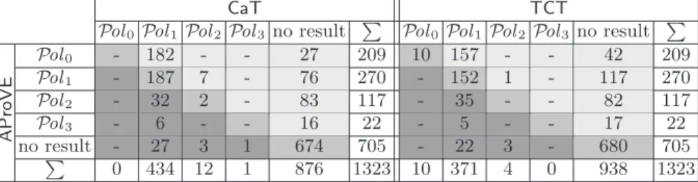
To evaluate our contributions, we implemented them in the termination pro- ver AProVE and compared it with the complexity tools CaT 1.5[27] and TCT 1.6[2]. We ran the tools on 1323 TRSs from theTermination Problem Data Base used in the International Termination Competition 2010.18 As in the competi- tion, each tool had a timeout of 60 seconds for each example. The left half of the
17One can also simplify (13) further by narrowing. Its subterm g♯(c(0, x)) has no narrowing substitutions. This (empty) set of narrowing substitutions captures f♯(h(c(0, x))) and h♯(c(0, x)) which have no narrowing substitutions either. Since f♯(x) is not captured, (13) can be transformed intof♯(c(0, x))→Com1(f♯(x)).
18Seehttp://www.termination-portal.org/wiki/Termination_Competition.
table comparesCaTandAProVE. For instance, the first row means thatAProVE showed constant complexity for 209 examples. On those examples, CaTproved linear complexity in 182 cases and failed in 27 cases. So in the light gray part of the table,AProVEgave more precise results thanCaT. In the medium gray part, both tools obtained equal results. In the dark gray part,CaTwas more precise thanAProVE. Similarly, the right half of the table comparesTCTandAProVE.
CaT TCT
Pol0 Pol1 Pol2 Pol3 no result P
Pol0 Pol1 Pol2 Pol3 no result P
AProVE
Pol0 - 182 - - 27 209 10 157 - - 42 209 Pol1 - 187 7 - 76 270 - 152 1 - 117 270 Pol2 - 32 2 - 83 117 - 35 - - 82 117 Pol3 - 6 - - 16 22 - 5 - - 17 22
no resultP - 27 3 1 674 705 - 22 3 - 680 705
0 434 12 1 876 1323 10 371 4 0 938 1323
So AProVE showed polynomial innermost runtime for 618 of the 1323 ex- amples (47 %). (Note that the collection also contains many examples whose complexity is not polynomial.) In contrast, CaT resp.TCT proved polynomial innermost runtime for 447 (33 %) resp. 385 (29 %) examples. Even a “combined tool” ofCaTandTCT(which always returns the better result of these two tools) would only show polynomial runtime for 464 examples (35 %). Hence, our contri- butions represent a significant advance. This also confirms the results of theTer- mination Competition 2010, where AProVEwon the category of innermost run- time complexity analysis.19 AProVEalso succeeds on Ex. 3, 25, and 37, whereas CaT and TCT fail. (Ex. 22 can be analyzed by all three tools.) For details on our experiments (including information on the exact DT processors used in each example) and to run our implementation inAProVEvia a web interface, we refer to http://aprove.informatik.rwth-aachen.de/eval/RuntimeComplexity/.
Acknowledgments.We are grateful to theCaTand theTCTteam for their support with the experiments and to G. Moser and H. Zankl for many helpful comments.
References
1. T. Arts and J. Giesl. Termination of term rewriting using dependency pairs. The- oretical Computer Science, 236:133–178, 2000.
2. M. Avanzini, G. Moser, and A. Schnabl. Automated implicit computational com- plexity analysis. InProc. IJCAR ’08, LNAI 5195, pages 132–138, 2008.
3. M. Avanzini and G. Moser. Dependency pairs and polynomial path orders. In Proc. RTA ’09, LNCS 5595, pages 48–62, 2009.
4. M. Avanzini and G. Moser. Closing the gap between runtime complexity and polytime computability. InProc. RTA ’10, LIPIcs 6, pages 33–48, 2010.
5. M. Avanzini and G. Moser. Complexity analysis by graph rewriting. In Proc.
FLOPS ’10, LNCS 6009, pages 257–271, 2010.
6. F. Baader and T. Nipkow. Term Rewriting and All That. Cambridge U. Pr., 1998.
7. G. Bonfante, A. Cichon, J.-Y. Marion, and H. Touzet. Algorithms with polynomial interpretation termination proof. J. Functional Programming, 11(1):33–53, 2001.
19In contrast to CaTand TCT,AProVEdid not participate in any other complexity categories as it cannot analyze derivational or non-innermost runtime complexity.
8. J. Endrullis, J. Waldmann, and H. Zantema. Matrix interpretations for proving termination of term rewriting.J. Automated Reasoning, 40(2-3):195–220, 2008.
9. A. Geser, D. Hofbauer, J. Waldmann, and H. Zantema. On tree automata that certify termination of left-linear term rewriting systems.Information and Compu- tation, 205(4):512–534, 2007.
10. J. Giesl, R. Thiemann, P. Schneider-Kamp. The DP framework: Combining tech- niques for automated termination proofs.LPAR ’04, LNAI 3452, p. 301–331, 2005.
11. J. Giesl, R. Thiemann, P. Schneider-Kamp, and S. Falke. Mechanizing and im- proving dependency pairs. Journal of Automated Reasoning, 37(3):155–203, 2006.
12. J. Giesl, M. Raffelsieper, P. Schneider-Kamp, S. Swiderski, and R. Thiemann.
Automated termination proofs forHaskellby term rewriting. ACM Transactions on Programming Languages and Systems, 33(2), 2011.
13. R. Givan and D. A. McAllester. Polynomial-time computation via local inference relations. ACM Transactions on Computational Logic, 3(4):521–541, 2002.
14. N. Hirokawa and A. Middeldorp. Automating the dependency pair method. In- formation and Computation, 199(1,2):172–199, 2005.
15. N. Hirokawa and G. Moser. Automated complexity analysis based on the depen- dency pair method. InProc. IJCAR ’08, LNAI 5195, pages 364–379, 2008.
16. N. Hirokawa and G. Moser. Complexity, graphs, and the dependency pair method.
InProc. LPAR ’08, LNAI 5330, pages 652–666, 2008.
17. D. Hofbauer and C. Lautemann. Termination proofs and the length of derivations.
InProc. RTA ’89, LNCS 355, pages 167–177, 1989.
18. M. Hofmann. Linear types and non-size-increasing polynomial time computation.
InProc. LICS ’99, pages 464–473. IEEE Press, 1999.
19. A. Koprowski and J. Waldmann. Max/plus tree automata for termination of term rewriting. Acta Cybernetica, 19(2):357–392, 2009.
20. J.-Y. Marion and R. P´echoux. Characterizations of polynomial complexity classes with a better intensionality. InProc. PPDP ’08, pages 79–88. ACM Press, 2008.
21. G. Moser, A. Schnabl, and J. Waldmann. Complexity analysis of term rewriting based on matrix and context dependent interpretations. InProc. FSTTCS ’08, LIPIcs 2, pages 304–315, 2008.
22. G. Moser. Personal communication, 2010.
23. F. Neurauter, H. Zankl, and A. Middeldorp. Revisiting matrix interpretations for polynomial derivational complexity of term rewriting. InProc. LPAR ’10, LNCS 6397, pages 550–564, 2010.
24. C. Otto, M. Brockschmidt, C. von Essen, J. Giesl. Automated termination analysis ofJava Bytecodeby term rewriting. InProc. RTA ’10, LIPIcs 6, pp. 259–276, 2010.
25. P. Schneider-Kamp, J. Giesl, T. Str¨oder, A. Serebrenik, and R. Thiemann. Auto- mated termination analysis for logic programs with cut. Proc. ICLP ’10, Theory and Practice of Logic Programming, 10(4-6):365–381, 2010.
26. J. Waldmann. Polynomially bounded matrix interpretations. In Proc. RTA ’10, LIPIcs 6, pages 357–372, 2010.
27. H. Zankl and M. Korp. Modular complexity analysis via relative complexity. In Proc. RTA ’10, LIPIcs 6, pages 385–400, 2010.
A Proofs
We first state a lemma with useful observations on ⊕, ⊖, and ιhD,S,Ri, which will be used throughout the proofs. Lemma 39 (a) and (b) shows that⊕and⊖ correspond to the addition and subtraction of functions (where for two functions f, g :N→N, we have (f +g)(n) = f(n) +g(n) and (f −g)(n) = max(f(n)− g(n),0)).
Moreover, the lemma shows the connection betweenιhD,S,Ri and the opera- tions⊕and⊖. For instance, for them-TRSRfrom Ex. 3 andD=DT(R), we haveιhD,D,Ri=Pol2. In Ex. 9 we also regarded the setSwhich contains all DTs except (6) – (8). We have irchD,S,Ri(n)∈ O(n) and thus, ιhD,S,Ri =Pol1. On the other hand, if one counts just the gt♯-DTs (6) – (8), then one again obtains irchD,D\S,Ri(n)∈ O(n2) and thus, ιhD,D\S,Ri =Pol2. So in particular, we have ιhD,S,Ri⊑ιhD,D,RiandιhD,D,Ri=ιhD,S,Ri⊕ιhD,D\S,Ri. These observations are generalized in Lemma 39 (g) and (h).
Lemma 39 (Properties of ⊕, ⊖, and ιhD,S,Ri). Let f and g be functions from NtoN∪ {ω} and letc, d, e∈C.
(a) ι(f)⊕ι(g) =ι(f +g) (b) ι(f)⊖ι(g)⊑ι(f −g)
(c) ⊕is associative and commutative (d) c⊖d⊑e iffc⊑d⊕e
(e) c⊖d⊒e does not implyc⊒d⊕e (f ) c⊒d⊕e does not implyc⊖d⊒e (g) IfS1⊆ S2 thenιhD,S1,Ri⊑ιhD,S2,Ri
(h) For anyS1,S2⊆ D, we have ιhD,S1,Ri⊕ιhD,S2,Ri=ιhD,S1∪S2,Ri
(i) For any S1,S2⊆ D, we have ιhD,S1,Ri⊖ιhD,S2,Ri⊑ιhD,S1\S2,Ri
Proof. For (a), ι(g) < ι(f) implies ι(f +g) = ι(f) and ι(f) ⊑ ι(g) implies ι(f +g) =ι(g).
For (b), first letι(f)⊑ι(g). Thenι(f)⊖ι(g) =Pol0⊑ι(f−g). Ifι(g)<ι(f) thenι(f)⊖ι(g) =ι(f) =ι(f−g).
The claim in (c) is obvious, since the “maximum” function onCis associative and commutative.
For (d), ifc⊑d, we have bothc⊖d=Pol0⊑eandc⊑d⊑d⊕e. Otherwise, letd<c. Ifd⊑e, we havec⊖d=c⊑eiffc⊑d⊕e=e. Ife<d, thend<c implies thatc⊖d=c⊑eis false. Similarly, then c⊑d⊕e=dis also false.
For (e), letc=e=Pol0andd=Pol1. Then we havec⊖d=Pol0⊖Pol1= Pol0⊒ Pol0=e, butc=Pol06⊒ Pol1=Pol1⊕ Pol0=d⊕e.
For (f), letc=d=e=Pol1. Then we have c=Pol1⊒ Pol1⊕ Pol1=d⊕e, but c⊖d=Pol1⊖Pol1=Pol06⊒ Pol1=e.
For (g), S1 ⊆ S2 implies that CplxhD,S1,Ri(t♯) ≤ CplxhD,S2,Ri(t♯) for any t♯ ∈ T♯. This implies irchD,S1,Ri(n) ≤ irchD,S2,Ri(n) for all n ∈ N and thus, ιhD,S1,Ri=ι(irchD,S1,Ri)⊑ι(irchD,S2,Ri) =ιhD,S2,Ri.
For (h), consider an arbitraryt♯∈ T♯. Letmbe the maximal number of nodes fromS1∪ S2occurring in any (D,R)-chain tree fort♯, i.e.,CplxhD,S1∪S2,Ri(t♯) =