EUROPEAN ORGANIZATION FOR NUCLEAR RESEARCH
Determination of α S using OPAL hadronic event shapes at
√ s = 91 − 209 GeV and resummed NNLO calculations
The OPAL Collaboration
Abstract
Hadronic event shape distributions from e+e− annihilation measured by the OPAL ex- periment at centre-of-mass energies between 91 GeV and 209 GeV are used to determine the strong coupling αS. The results are based on QCD predictions complete to the next- to-next-to-leading order (NNLO), and on NNLO calculations matched to the resummed next-to-leading-log-approximation terms (NNLO+NLLA). The combined NNLO result from all variables and centre-of-mass energies is
αS(mZ0) = 0.1201±0.0008(stat.)±0.0013(exp.)±0.0010(had.)±0.0024(theo.).
while the combined NNLO+NLLA result is
αS(mZ0) = 0.1189±0.0008(stat.)±0.0016(exp.)±0.0010(had.)±0.0036(theo.).
The completeness of the NNLO and NNLO+NLLA results with respect to missing higher order contributions, studied by varying the renormalization scale, is improved compared to previous results based on NLO or NLO+NLLA predictions only. The observed energy dependence of αS agrees with the QCD prediction of asymptotic freedom and excludes the absence of running.
(To be submitted to European Physical Journal C) final draft
January 7, 2011
The OPAL Collaboration
G. Abbiendi2, C. Ainsley5,u, P.F. ˚Akesson7, G. Alexander21, G. Anagnostou1, K.J. Anderson8, S. Asai22, D. Axen26, I. Bailey25,g, E. Barberio7,o, T. Barillari31, R.J. Barlow15, R.J. Batley5, P. Bechtle24, T. Behnke24, K.W. Bell19, P.J. Bell1, G. Bella21,
A. Bellerive6, G. Benelli4,j, S. Bethke31, O. Biebel30, O. Boeriu9, P. Bock10, M. Boutemeur30, S. Braibant2, R.M. Brown19, H.J. Burckhart7, S. Campana4,x,
P. Capiluppi2, R.K. Carnegie6, A.A. Carter12, J.R. Carter5, C.Y. Chang16,
D.G. Charlton1, C. Ciocca2, A. Csilling28, M. Cuffiani2, S. Dado20, M. Dallavalle2, A. De Roeck7, E.A. De Wolf7,r, K. Desch24, B. Dienes29, J. Dubbert30,f, E. Duchovni23, G. Duckeck30, I.P. Duerdoth15, E. Etzion21, F. Fabbri2, P. Ferrari7, F. Fiedler30, I. Fleck9,
M. Ford15, A. Frey7, P. Gagnon11, J.W. Gary4, C. Geich-Gimbel3, G. Giacomelli2, P. Giacomelli2, M. Giunta4,a4, J. Goldberg20, E. Gross23, J. Grunhaus21, M. Gruw´e7,
A. Gupta8, C. Hajdu28, M. Hamann24, G.G. Hanson4, A. Harel20, M. Hauschild7, C.M. Hawkes1, R. Hawkings7, G. Herten9, R.D. Heuer7, J.C. Hill5, D. Horv´ath28,c, P. Igo-Kemenes10, K. Ishii22,t, H. Jeremie17, P. Jovanovic1, T.R. Junk6,a3, J. Kanzaki22,t,
D. Karlen25, K. Kawagoe22, T. Kawamoto22, R.K. Keeler25, R.G. Kellogg16, B.W. Kennedy19, S. Kluth31, T. Kobayashi22, M. Kobel3,s, S. Komamiya22, T. Kr¨amer24,
A. Krasznahorkay Jr.29,e, P. Krieger6,k, J. von Krogh10, T. Kuhl24, M. Kupper23, G.D. Lafferty15, H. Landsman20, D. Lanske13,∗, D. Lellouch23, J. Lettsn, L. Levinson23,
J. Lillich9, S.L. Lloyd12, F.K. Loebinger15, J. Lu26,b, A. Ludwig3,s, J. Ludwig9, W. Mader3,s, S. Marcellini2, A.J. Martin12, T. Mashimo22, P. M¨attigl, J. McKenna26,
R.A. McPherson25, F. Meijers7, W. Menges24, F.S. Merritt8, H. Mes6,a, N. Meyer24, A. Michelini2, S. Mihara22,t, G. Mikenberg23, D.J. Miller14, W. Mohr9, T. Mori22, A. Mutter9, K. Nagai12,a2, I. Nakamura22,t, H. Nanjo22,v, H.A. Neal32, S.W. O’Neale1,∗, A. Oh7, M.J. Oreglia8, S. Orito22,∗, C. Pahl31, G. P´asztor4,a5, J.R. Pater15, J.E. Pilcher8,
J. Pinfold27, D.E. Plane7, O. Pooth13, M. Przybycie´n7,m, A. Quadt31, K. Rabbertz7,q, C. Rembser7, P. Renkel23, J.M. Roney25, A.M. Rossi2, Y. Rozen20, K. Runge9, K. Sachs6,
T. Saeki22,t, E.K.G. Sarkisyan7,i, A.D. Schaile30, O. Schaile30, P. Scharff-Hansen7, J. Schieck31,z, T. Sch¨orner-Sadenius7,y, M. Schr¨oder7, M. Schumacher3, R. Seuster13,f,
T.G. Shears7,h, B.C. Shen4,∗, P. Sherwood14, A. Skuja16, A.M. Smith7, R. Sobie25, S. S¨oldner-Rembold15, F. Spano8,w, A. Stahl13, D. Strom18, R. Str¨ohmer30,a1, S. Tarem20,
M. Tasevsky7,d, R. Teuscher8,k, M.A. Thomson5, E. Torrence18, D. Toya22, I. Trigger7,a, Z. Tr´ocs´anyi29,e, E. Tsur21, M.F. Turner-Watson1, I. Ueda22, B. Ujv´ari29,e, C.F. Vollmer30,
P. Vannerem9, R. V´ertesi29,e, M. Verzocchi16, H. Voss7,p, J. Vossebeld7,h, C.P. Ward5, D.R. Ward5, P.M. Watkins1, A.T. Watson1, N.K. Watson1, P.S. Wells7, T. Wengler7, N. Wermes3, G.W. Wilson15,j, J.A. Wilson1, G. Wolf23, T.R. Wyatt15, S. Yamashita22,
D. Zer-Zion4, L. Zivkovic20
1School of Physics and Astronomy, University of Birmingham, Birmingham B15 2TT, UK
2Dipartimento di Fisica dell’ Universit`a di Bologna and INFN, I-40126 Bologna, Italy
3Physikalisches Institut, Universit¨at Bonn, D-53115 Bonn, Germany
4Department of Physics, University of California, Riverside CA 92521, USA
5Cavendish Laboratory, Cambridge CB3 0HE, UK
6Ottawa-Carleton Institute for Physics, Department of Physics, Carleton University, Ot- tawa, Ontario K1S 5B6, Canada
7CERN, European Organisation for Nuclear Research, CH-1211 Geneva 23, Switzerland
8Enrico Fermi Institute and Department of Physics, University of Chicago, Chicago IL 60637, USA
9Fakult¨at f¨ur Physik, Albert-Ludwigs-Universit¨at Freiburg, D-79104 Freiburg, Germany
10Physikalisches Institut, Universit¨at Heidelberg, D-69120 Heidelberg, Germany
11Indiana University, Department of Physics, Bloomington IN 47405, USA
12Queen Mary and Westfield College, University of London, London E1 4NS, UK
13Technische Hochschule Aachen, III Physikalisches Institut, Sommerfeldstrasse 26-28, D- 52056 Aachen, Germany
14University College London, London WC1E 6BT, UK
15School of Physics and Astronomy, Schuster Laboratory, The University of Manchester M13 9PL, UK
16Department of Physics, University of Maryland, College Park, MD 20742, USA
17Laboratoire de Physique Nucl´eaire, Universit´e de Montr´eal, Montr´eal, Qu´ebec H3C 3J7, Canada
18University of Oregon, Department of Physics, Eugene OR 97403, USA
19Rutherford Appleton Laboratory, Chilton, Didcot, Oxfordshire OX11 0QX, UK
20Department of Physics, Technion-Israel Institute of Technology, Haifa 32000, Israel
21Department of Physics and Astronomy, Tel Aviv University, Tel Aviv 69978, Israel
22International Centre for Elementary Particle Physics and Department of Physics, Uni- versity of Tokyo, Tokyo 113-0033, and Kobe University, Kobe 657-8501, Japan
23Particle Physics Department, Weizmann Institute of Science, Rehovot 76100, Israel
24Universit¨at Hamburg/DESY, Institut f¨ur Experimentalphysik, Notkestrasse 85, D-22607 Hamburg, Germany
25University of Victoria, Department of Physics, P O Box 3055, Victoria BC V8W 3P6, Canada
26University of British Columbia, Department of Physics, Vancouver BC V6T 1Z1, Canada
27University of Alberta, Department of Physics, Edmonton AB T6G 2J1, Canada
28Research Institute for Particle and Nuclear Physics, H-1525 Budapest, P O Box 49, Hungary
29Institute of Nuclear Research, H-4001 Debrecen, P O Box 51, Hungary
30Ludwig-Maximilians-Universit¨at M¨unchen, Sektion Physik, Am Coulombwall 1, D-85748 Garching, Germany
31Max-Planck-Institute f¨ur Physik, F¨ohringer Ring 6, D-80805 M¨unchen, Germany
32Yale University, Department of Physics, New Haven, CT 06520, USA
a and at TRIUMF, Vancouver, Canada V6T 2A3
b now at University of Alberta
c and Institute of Nuclear Research, Debrecen, Hungary
d now at Institute of Physics, Academy of Sciences of the Czech Republic 18221 Prague,
Czech Republic
e and Department of Experimental Physics, University of Debrecen, Hungary
f now at MPI M¨unchen
g now at Lancaster University
h now at University of Liverpool, Dept of Physics, Liverpool L69 3BX, U.K.
i now at University of Texas at Arlington, Department of Physics, Arlington TX, 76019, U.S.A.
j now at University of Kansas, Dept of Physics and Astronomy, Lawrence, KS 66045, U.S.A.
k now at University of Toronto, Dept of Physics, Toronto, Canada
l now at Bergische Universit¨at, Wuppertal, Germany
m now at University of Mining and Metallurgy, Cracow, Poland
n now at University of California, San Diego, U.S.A.
o now at The University of Melbourne, Victoria, Australia
p now at IPHE Universit´e de Lausanne, CH-1015 Lausanne, Switzerland
q now at IEKP Universit¨at Karlsruhe, Germany
r now at University of Antwerpen, Physics Department,B-2610 Antwerpen, Belgium; sup- ported by Interuniversity Attraction Poles Programme – Belgian Science Policy
s now at Technische Universit¨at, Dresden, Germany
t and High Energy Accelerator Research Organisation (KEK), Tsukuba, Ibaraki, Japan
u now at University of Pennsylvania, Philadelphia, Pennsylvania, USA
v now at Department of Physics, Kyoto University, Kyoto, Japan
w now at Columbia University
x now at CERN
y now at DESY
z now at Ludwig-Maximilians-Universit¨at M¨unchen, Germany
a1 now at Julius-Maximilians-University W¨urzburg, Germany
a2 now at University of Tsukuba, Japan
a3 now at FERMILAB
a4 now at Universit`a di Bologna and INFN
a5 now at University of Geneva
a6 now at Georg-August University of G¨ottingen
∗ Deceased
1 Introduction
Events originating from e+e− annihilation into quark-antiquark pairs allow precision tests [1–3] of the theory of the strong interaction, Quantum Chromodynamics (QCD) [4–
7]. Comparison of observables like jet production rates or event shape variables with theoretical predictions allows the crucial free parameter of QCD – the strong couplingαS – to be determined. The determination ofαS from many different observables provides an important consistency test of QCD. Recently, significant progress in the theoretical calcu- lation of event shape observables has been made. Next-to-next-to-leading order (NNLO) calculations are now available [8,9] as well as NNLO calculations matched with resummed terms in the next-to-leading-logarithmic-approximation (NLLA) [10].
Measurements of αS at centre-of-mass-system (c.m.) energies between √
s = 91 GeV and 206 GeV, using NNLO predictions and ALEPH data, were presented in [11]. This was followed by measurements between√
s = 14 GeV and√
s= 44 GeV [12] and between
√s = 91 GeV and √
s = 206 GeV [13] based on comparing JADE or ALEPH data with NNLO plus matched NLLA calculations. The strong coupling has also been determined at NNLO from the three-jet rate at LEP [14]. In the present study, the revised NNLO calculations described in [8, 9] are used to determine αS at NNLO and NNLO+NLLA for 13 different energy values between 91 and 209 GeV. The data sample is that of the OPAL Collaboration at LEP. Hadronization corrections are treated in the manner described in [2, 11, 12, 15]. The study is based on the same measurements of event shape variables, the same fit ranges (except fory23D as discussed below), and the same Monte Carlo models for detector and hadronization corrections as those in [15].
The structure of the paper is as follows. In Sect. 2 we give an overview of the OPAL detector, and in Sect. 3 we summarize the data and Monte Carlo samples used. The theoretical background to the work is outlined in Sect. 4. The experimental analysis techniques are explained in Sect. 5, and the measurements are compared with theory in Sect. 6.
2 The OPAL Detector
The OPAL experiment operated from 1989 to 2000 at the LEP e+e− collider at CERN.
The OPAL detector is described in detail in [16–18]. This analysis mostly makes use of the measurements of energy deposited in the electromagnetic calorimeter and of charged particle momenta in the tracking chambers.
All tracking systems were located inside a solenoidal magnet, which provided a uniform axial magnetic field of 0.435 T along the beam axis. The main tracking detector was the central jet chamber. This device was approximately 4 m long and had an outer radius of about 1.85 m. The magnet was surrounded by a lead glass electromagnetic calorimeter and a sampling hadron calorimeter. The electromagnetic calorimeter consisted of 11704 lead glass blocks, covering 98% of the solid angle. Outside the hadron calorimeter, the detector was surrounded by a system of muon chambers.
3 Data and Monte Carlo Samples
The analysis is based on the same data, Monte Carlo samples, and event selection, as those employed in a previous study [15]. The data were collected at c.m. energies be- tween 91.0 GeV and 208.9 GeV. The data at 91 GeV, on the Z0 peak, were collected during calibration runs between 1996 and 2000 and have the same conditions of detector configuration, performance and software reconstruction as the higher energy data. The data are grouped into samples with similar c.m. energies, as indicated in Tab. 1. Be- sides the energy range, mean energy and integrated luminosity, Tab. 1 lists the year(s) of collection and the number of selected hadronic annihilation events for each sample.
Samples of Monte Carlo-simulated events were used to correct the data for experi- mental acceptance, efficiency and backgrounds. The e+e− → qq process was simulated at √
s = 91.2 GeV using JETSET 7.4 [19], and at higher energies using KK2f 4.01 or KK2f 4.13 [20, 21] with hadronization performed using PYTHIA 6.150 or PY- THIA 6.158 [19]. Corresponding samples of HERWIG 6.2 [22, 23] or KK2f events with HERWIG 6.2 hadronization were used for systematic checks. Four-fermion background processes were simulated using grc4f 2.1 [24], KORALW 1.42 [25] with grc4f [24] matrix elements, with hadronization performed using PYTHIA. The above samples, generated at each energy point studied, were processed through a full simulation of the OPAL detector [26] and reconstructed in the same manner as the data. In addition, when correcting for the effects of hadronization, large samples of generator-level Monte Carlo events were employed, using the parton shower models PYTHIA 6.158, HERWIG 6.2 and ARIADNE 4.11 [27].
Each of these models used for the description of hadronization and detector response contains a number of tunable parameters. These parameters were adjusted to describe previously published OPAL data at √
s ∼ 91 GeV as discussed in [28] for PYTHIA/
JETSET and in [29] for HERWIG and ARIADNE.
4 Theoretical Background
4.1 Event Shape Distributions
The properties of hadronic events can be described by event shape observables. The event shape observables used for this analysis are thrust (1−T) [30, 31], heavy jet mass (MH) [32], wide and total jet broadening (BW and BT) [33], C-Parameter (C) [34–36]
and the transition value between 2 and 3 jet configurations defined using the Durham jet algorithm (y23D) [37].
In the following, the symbol y is used to refer to any of the variables 1−T,MH,BT, BW, C ory23D. Event shape variables characterize the main features of the distribution of momentum in an event. Larger values ofy correspond to the multi-jet region dominated by the radiation of hard gluons. Smaller values ofy correspond to the two-jet region with only soft and collinear radiation.
4.2 QCD Calculations
QCD predictions for the distribution of event shape observables in e+e− annihilations are now available to O(α3S) (NNLO) [8, 9]. In the case where the renormalization scale µR
equals the physical scale Q identified with√
s, the predictions are:
1 σ
dσ dy O
(α3S)
= dA
dyαˆS+dB
dyαˆ2S+dC
dyαˆ3S (1)
with ˆαS =αS(µR)/(2π). The coefficient distributions for the leading order (LO) dA/dy, next-to-leading order (NLO) dB/dy and NNLO dC/dy terms were provided to us by the authors of [8]. The normalization to the total hadronic cross section and the terms generated by variation of the renormalization scale parameterxµ =µR/Qare implemented according to the prescription of [8].
In the two-jet (lowy) region, the effect of soft and collinear emissions introduces large logarithmic effects depending on L = log(1/y). For the (1−T), MH, BT, BW, C and yD23 distributions, the leading and next-to-leading logarithmic terms can be resummed up to infinite order in perturbation theory [38]. This is referred to as the next-to-leading- logarithmic approximation (NLLA). The most complete calculations of event shape ob- servables are obtained from combining (matching) the O(α3S) and NLLA calculations, taking care not to double count terms that are in common between them.
The matching is not unique. In the so-called lnRmatching scheme, the NNLO+NLLA expression for the logarithm of the cumulative distribution R(y) = Ry
0 dy′(1/σ)dσ/dy′ is [10]
ln (R(y,αˆS)) =L g1(ˆαSL) + g2( ˆαSL) (2) + αˆS A(y)−G11L−G12L2
+ αˆ2S
B(y)− 1
2A2(y)−G22L2 −G23L3
+ αˆ3S
C(y)−A(y)B(y) + 1
3A3(y)−G33L3−G34L4
.
The functions g1 and g2 represent the resummed leading and next-to-leading logarithmic terms while the Gij are matching coefficients. The coefficient functions A, B and C are related to the differential coefficients in (1) by integration, e.g. A(y) = Ry
0 dy′dA(ydy′′). Since αS in the NNLO and NLLA terms are assumed to be the same, there is only one renormalization scale. The NLLA terms introduce a further arbitrariness in the choice of a logarithmic rescaling variable xL, see [15].
The theoretical calculations provide distributions at the level of quarks and gluons, the so-called parton-level. Monte Carlo-based distributions calculated using the final- state partons after termination of the parton showering in the models are also said to be at the parton-level. In contrast, the data are corrected to the hadron-level, i.e. they corre- spond to the distributions of the stable particles in the event as explained in Sect. 5.2. To compare the QCD predictions with measured event shape distributions these predictions are corrected from the parton to the hadron level. The corrections are based on large samples of typically 107 events generated with the parton-shower Monte Carlo programs
PYTHIA (used by default), HERWIG and ARIADNE (used to evaluate systematic uncer- tainties). The corrections are defined by the ratio of the Monte Carlo distributions at the hadron and parton levels and are applied as multiplicative corrections to the theoretical predictions.
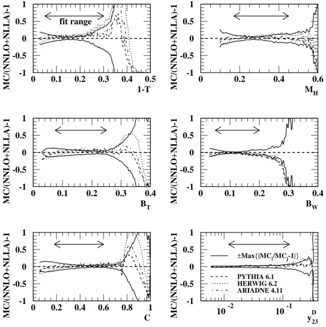
We compare the parton-level calculations of the Monte Carlo generators with the QCD calculations in NNLO+NLLA with αS(mZ0) = 0.118, xµ = 1.0 and xL = 1.0 at
√s = 91 GeV, see Fig. 1 and [12]. The dashed line shows the deviation from one of the ratio between the Pythia prediction at the parton level and the NNLO+NLLA calculation.
The dotted (dash-dotted) line shows the corresponding result from Herwig (Ariadne).
The solid lines, symmetric about zero, show the maximum difference between any pair of the Monte Carlo models, which are seen to be of similar size to the differences between the generators and the NNLO+NNLA calculation. Therefore we consider that the MC simulations adequately account for the hadronization correction to the calculations.
The model dependence of the hadronization correction is included as a systematic uncertainty as described below.
5 Experimental Procedure
The data used in the present paper are identical to those presented in [15, 39, 40]. For completeness and to facilitate the discussion of systematic uncertainties, we give a brief summary of the analysis procedure below.
5.1 Event Selection
The event selection procedure is described in [15]. This procedure selects well-measured hadronic event candidates, removes events with a large amount of initial-state radiation (ISR) at 130 GeV and above, and removes four-fermion background events above the W+W− production threshold of 160 GeV.
5.2 Corrections to the Data
For each accepted event, the value of each event shape observable is computed. A standard algorithm [41] is applied to mitigate the double-counting of energy between the tracking chambers and calorimeter. To correct for background contributions, the expected number of residual four-fermion events bi is subtracted from the number of data eventsNi in each biniof each distribution. Simple bin-by-bin corrections are applied to account for detector acceptance, resolution, and the effects of residual ISR. We examine the Monte Carlo predictions for the event shape variables at two levels: the detector level, which includes simulation of the detector and the same analysis procedures as applied to the data, and the hadron level, which uses stable particles1 only, assumes perfect reconstruction of the particle momenta, and requires the hadronic c.m. energy√
s′ to satisfy√ s−√
s′ <1 GeV.
The ratio of the hadron- to the detector-level prediction for each bin, αi, is used as the correction factor for the data, yielding the corrected bin content Nei = αi(Ni −bi).
1For this purpose, all particles having proper lifetimes greater than 3×10⁻¹⁰s are regarded as stable.
This corrected hadron-level distribution is then normalized by the total number of events N =P
kNek and bin width Wi: Pi =Nei/(NWi).
5.3 Systematic uncertainties
To evaluate systematic uncertainties, the analysis is repeated after modifying the selection or correction procedures. The event and track selection cuts are varied within the ranges of values suggested in [15]. The Monte Carlo model employed to calculate the detector correction is altered, and the cross section used in the subtraction of four-fermion events is varied by ±5%. In each case, the difference in each bin with respect to the standard analysis is taken as a contribution to the systematic uncertainty.
6 Determinations of αS
6.1 Fit procedure
The strong couplingαSis determined using a minimum-χ2 fit, comparing theory with each of the measured event shape distributions at the hadron level. A χ2 value is calculated at each c.m. energy:
χ2 = Xn
i,j
(Pi−ti(αS))(V−1)ij(Pj −tj(αS)) (3)
where i, j include the bins within the fit range of the event shape distribution, Pi is the measured value in the ith bin, ti(αS) is the QCD prediction for the ith bin corrected for hadronization effects, and V−1 is the inverse of the statistical covariance matrix Vstat of the values Pi. The QCD prediction is obtained by integrating the result in (1) over the bin width, and then applying the hadronization correction. The χ2 value is minimized with respect toαS with the renormalization scale factor xµ and the rescaling variablexL set to 1. The evolution of the strong couplingαSas a function of the renormalization scale is implemented to three-loop order [42]. Since the c.m. energy range considered here does not cross flavour thresholds, no significant uncertainties are introduced by the evolution ofαS. Separate fits are performed to each of the six observables at each c.m. energy value.
To account for correlations between bins in the computation of χ2, the statistical covariance matrix Vijstat is calculated following the approach described in [15]:
Vijstat = X
k
∂Pi
∂Nk
∂Pj
∂Nk
Nk (4)
= 1
N4 X
k
α2kNk
Nδik−Nei Nδjk−Nej
.
where δik is the Kronecker delta function, and the other terms are defined in Sect. 5.2.
To test our procedure, we verified that we are able to reproduce the fit results from [15, 43] using NLO+NLLA predictions within typically 0.5%.
The fit ranges are chosen as in [15,44] and correspond to regions where the corrections of the data and of the parton level theory to the hadron level are both reasonably small and where the NLO+NLLA fit results are stable under small variations of the fit range.
The relevant calculations in the two-jet region are the NLLA terms, which are identical in the present study and [15]. The NNLO prediction for y23D is given in bins of −lny23D. The transformation to bins of y23D produces precision problems for small values of y23D. Therefore we use a more restrictive fit range for y23D than in [15], which approximately matches the range in [12]: the lower bound is 0.012 rather than 0.0023.
The fit ranges are shown in Tab. 2. In the resummation of log-enhanced terms, the leading log term of dA/dy is ln(y)/y. At y values equal to the lower limit y0, the value of ˆαSln(y0)/y0 is still of the order of one for αS(mZ0) = 0.118 and 91 ≤√
s ≤ 207 GeV.
Thus the fit ranges are also suitable for pure NNLO analysis.
Previously measured event shape distributions are published [15] only in the energy ranges as separated by horizontal lines in Tab. 1. We perform fits to extract αS at all of the energy points2 shown in Tab. 1 column 2. We average over the larger energy ranges only for purposes of presentation.
The detector correction factors are typically between 0.9 and 1.5 within the fit ranges.
For energies above 189 GeV, which have low statistics, the corrections exceed 2.0 in the multi-jet regions. The maximum correction of 4.8 occurs for the 1−T distribution at 207 GeV. The variable with the least variation in the size of its hadronization correction, and with hadronization corrections closest to one, is y23D.
The statistical uncertainty of αS is given by the variation required to increase χ2 by one unit from its minimum. The systematic uncertainties account for experimental effects, the hadronization correction procedure and uncertainties of the theory. The three sources of systematic uncertainty are added in quadrature to the statistical uncertainty to define the total uncertainty. Below, we describe the evaluation of systematic uncertainties. For each variant of the analysis, the corresponding distribution is fitted to determine αS, and the difference with respect to the value of αS from the default analysis is taken as a systematic uncertainty contribution.
Experimental Uncertainties: These are assessed as described in Sect. 5.3.
Hadronization: For the default analysis, PYTHIA is used to evaluate hadronization corrections (Sect. 4.2). As systematic variations, HERWIG and ARIADNE are used instead. The larger of the deviations is taken as the systematic uncertainty. It was observed in [45, 46] that systematic uncertainties determined from the differences between the PYTHIA, HERWIG, and ARIADNE models are generally much larger than those that arise from varying the parameters of a given model.
Theoretical Uncertainties: The theoretical calculation of event shape observables is a finite power series in αS. The uncertainties originating from missing higher order terms are assessed by changing the renormalization scale factor to xµ = 0.5 and xµ = 2.0. The rescaling variable is set to xL = 2/3 and xL = 3/2 (xL = 4/9 and xL = 9/4 in case of y23D) [15]. The largest deviation with respect to the standard
2This allows the use of the event shape covariance matrices which are energy dependent and have been calculated separately for each energy point.
analysis is taken as the systematic uncertainty. A variation of the matching scheme is not studied because R-matching is not available for NNLO+NLLA. The match- ing scheme was not an important source of uncertainty in studies of αS based on NLO+NLLA calculations.
6.2 Results from NNLO Fits
The results of the NNLO fits are summarised in Tab. 3. In order to clarify the presenta- tion, the αS values from 130 and 136 GeV are combined3, and likewise the values from 161 to 183 GeV, and from 189 GeV and above. These three ranges of c.m. energies, which correspond to luminosity weighted mean energies of 133.1, 177.4 and 197.0 GeV, respectively, cover sufficiently small ranges of √
s that only small variations of αS occur within each range.
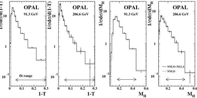
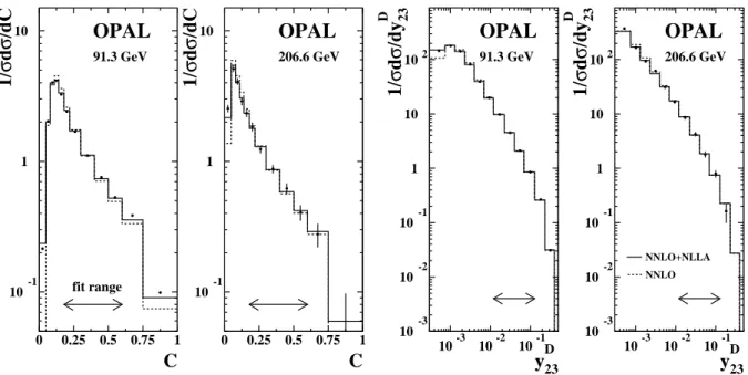
Figs. 2, 3 and 4 show the 1−T, MH, BT, BW, C and y23D event shape distributions together with the NNLO fit results for the 91.3 and 206.6 GeV energy points. All event shape distributions are described reasonably well by the fitted predictions. The χ2/d.o.f. values, which are large for the data at the Z0 peak because they are based on statis- tical uncertainties only, range from 0.03 for y23D at √
s = 191.6 GeV to 228 for BT at
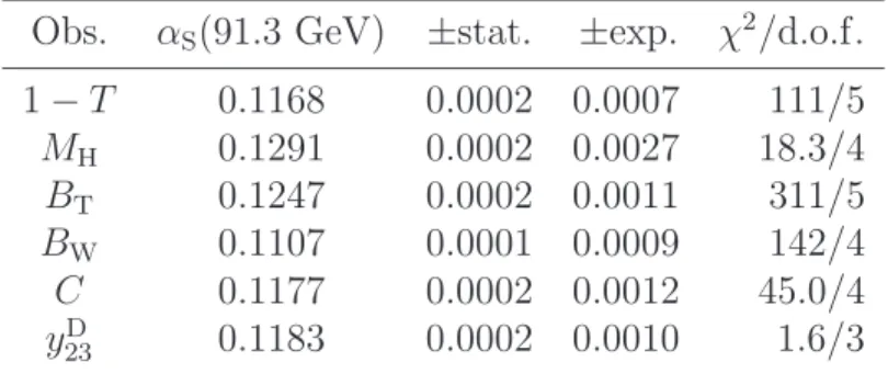
√s = 91.3 GeV. The uncertainties at this point are dominated by the experimental sys- tematic uncertainties (discussed below). To check how the inclusion of the experimental errors in the fits reduces the large χ2 values, an alternative χ2 value is defined as fol- lows. An estimate of the experimental systematic covariance is added to the statistical covariance (4),
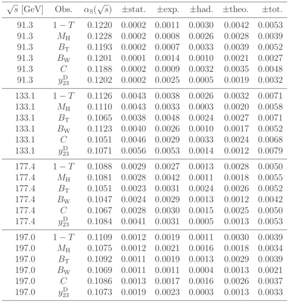
Vijtotal=Vijstat+ min(σ2exp,i, σ2exp,j), (5) where σexp,i is the experimental systematic uncertainty at bin i. Tab. 4 shows the fit results at 91 GeV. The fit results are in general not compatible within the combined statistical and experimental errors with the results when only the statistical covariance is used. These χ2/d.o.f. values are smaller than those from employing the statistical covariances, however they still range up to 62 for BT. We return to this issue when we discuss the NNLO+NLLA fits below.
The results for αS from the different event shape variables are remarkably consistent with each other, for each c.m. energy, as seen from Tabs. 10, 11 (but not in the case of the modified fit procedure whose results are shown in Tab. 4). We find root-mean-square (r.m.s.) values for αS(√
s) between 0.0012 at 183 GeV and 0.0044 at 202 GeV. The variations in αS between the different variables are comparable to the total systematic uncertainties. The values ofαS are significantly larger at 91 GeV than at higher energies, providing evidence for the running of αS. Theoretical uncertainties dominate at the Z0peak (except fory23D), where the statistical uncertainties are small. Similarly, statistical uncertainties are small at 189 GeV where there is a relatively large data sample. Statistical uncertainties dominate at 130, 161 and 172 GeV, where the data samples are smaller.
Experimental systematic uncertainties are small at 91 GeV and larger at higher√
swhere
3This combination is performed assuming minimum overlap correlation of the experimental uncertain- ties at the different c.m. energy points. The procedure includes a correction for the running ofαS(√s) to the luminosity weighted mean energy.
uncertainties from subtraction of ISR and four fermion events contribute more strongly.
For completeness, the fit results for all energy points are given separately in App. A.
6.3 Results from NNLO+NLLA Fits
The results of the NNLO+NLLA fits are shown in Figs. 2, 3 and 4 and listed in Tab. 5.
The calculations fit the data better than the pure NNLO calculations at small values of the variables. The values of χ2/d.o.f. are smaller on average than for the NNLO fits, especially at 91 GeV, indicating better consistency with the data. The r.m.s. values of αS(√
s) vary between 0.0017 at √
s = 205 GeV and 0.0051 at √
s = 202 GeV, i.e. the scatter of individual results is essentially the same as for the NNLO analysis. The pattern of statistical, experimental, and hadronization uncertainties is the same as for the NNLO fits discussed above. At most energy points the theory error results from thexL variation forMH,BW, yD23, and from thexµ variation for 1−T,BT, C. Compared with the NNLO analysis the values of αS are lower by 0.4% on average, and the theoretical uncertainties are higher by 33%. Larger scale uncertainties are expected to arise at 91 GeV when the NLLA terms are added to the NNLO terms [10, 13, 47], because the NNLO calculation compensates for the variation of the renormalization scale in two loops, while the NLLA term compensates for the variation in only one loop. The difference we observe between αS in the NNLO and NNLO+NLLA studies is smaller than the corresponding difference observed between the NLO and NLO+NLLA studies (Sect. 6.5), as predicted in [10]. This difference is also smaller than that observed at lower energies [12], as expected from the energy evolution of αS.
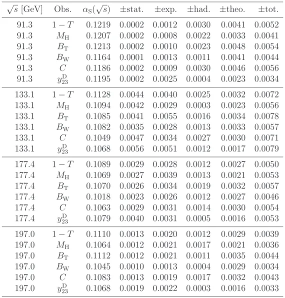
The fit results at 91 GeV employing the total covariance (5) are shown in Tab. 6.
Unlike the case of pure NNLO, the fit results are compatible with the results based on only the statistical covariance within the combined statistical and experimental systematic uncertainties. The χ2/d.o.f. values are of the order of 1. For a reasonable description of the data by the theory predictions, inclusion of the resummed logarithmic terms (NLLA) is seen to be important. As the covariance (5) is only an approximation, we do not use the fit values or errors further.
6.4 Combination of Results
The results obtained at each energy point for the six event shape observables are com- bined using uncertainty-weighted averaging as in [2,15,48,49]. The statistical correlations between the six event shape observables are estimated at each energy point from fits to hadron-level distributions derived from 50 statistically-independent Monte Carlo samples.
The experimental uncertainties are determined assuming that the smaller of a pair of cor- related experimental uncertainties gives the size of the fully correlated uncertainty. The minimum overlap assumption results in a conservative estimate of the total uncertainty.
The hadronization and theoretical systematic uncertainties are evaluated by repeating the combination with changed input values, i.e. using a different hadronization model or the different value of xµ or xL that yields the maximum deviation. The results are given in Tab. 7 and shown for the NNLO+NLLA analysis in Fig. 5. Also shown is a comparison with the results of a NNLO+NLLA analysis at lower energy from the JADE
Collaboration [12].
To study the compatibility of our data with the QCD prediction for the evolution of the strong coupling with c.m. energy we repeat the combinations with or without evolution of the combined results to the common scale, setting the theory uncertainties to zero since these uncertainties are highly correlated between energy points. We assume the hadronization uncertainties to be partially correlated. The χ2 probability of the average for a running (constant) coupling in the NNLO+NLLA study is 0.59 (6×10⁻¹³). The corresponding result for the NNLO study is 0.56 (2×10⁻⁶). We interpret this as clear evidence, from OPAL data alone, for the running ofαS in the manner predicted by QCD.
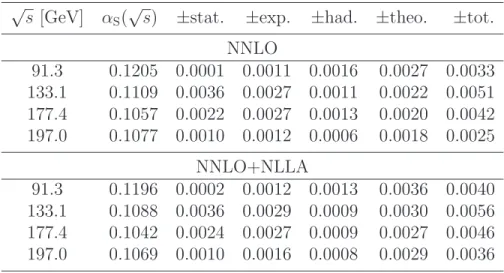
We evolve the results in Tab. 7 with √
s > mZ0 to a common scale mZ0 using the QCD formula for the running ofαS. The results are then combined using the uncertainty- weighted averaging procedure mentioned above. The results are shown in Tab. 8 for the NNLO and NNLO+NLLA analyses. The consistency between these values and the results from 91 GeV (Tab. 7) demonstrates the compatibility of the data with the running predicted by QCD. The high energy data have smaller theoretical and hadronization uncertainties, and therefore complement the statistically superior 91 GeV data.
The values of αS(mZ0) obtained from combining all energy points are also given in Tab. 8. The resulting values of αS(mZ0) = 0.1201±0.0031 from the NNLO study, and αS(mZ0) = 0.1189±0.0041 from the NNLO+NLLA study, are consistent with the world average [50] (0.1184 ±0.0007), recent NNLO analyses of JADE [12] (0.1172 ±0.0051) and ALEPH [11] (0.1240±0.0033) data, our previous study [15] based on NLO+NLLA calculations (0.1191±0.0047) and the study [13] of ALEPH data using NNLO+NLLA (0.1224± 0.0039). The total uncertainties of 2.6% and 3.4% for αS(mZ0) place these measurements amongst the most precise determinations of αS available.
After running the fit results for αS(√
s) for each observable to the common reference scale mZ0, we combine the results for a given observable to a single value. We use the same method as above and obtain the results forαS(mZ0) shown in Tab. 9. These results demonstrate that the measurements from the different observables are far from compatible with each other when only statistical uncertainties are considered, but are consistent with a common mean when the systematic uncertainties are included, neglecting their correla- tion. The r.m.s. values of the results for αS(mZ0) are 0.0013 for the NNLO analysis and 0.0026 for the NNLO+NLLA analysis; both values lie within the range of the uncertainty for the corresponding combined result shown in Tab. 8. Fig. 6 displays the combined αS result for each observable. Results from NLO and NLO+NLLA studies, discussed below, are also shown. Combining the NNLO or NNLO+NLLA results of Fig. 6 to obtain an overall value for αS, or evolving each event shape measurement from each energy to the reference scale and then combining, yields the same result as given by the corresponding measurement in Tab. 8 to within ∆αS(mZ0) = 0.0003.
6.5 Comparison with NLO and NLO+NLLA fits
To compare our results with previousαS measurements, the fits to the event shape distri- butions are repeated with NLO predictions and with NLO predictions combined with resummed NLLA with the modified lnR-matching scheme (NLO+NLLA), both with xµ= 1. The NLO+NLLA calculations with the modified lnR-matching scheme were the
standard of the analyses at the time of termination of the LEP experiments [15,49,51,52].
The fit ranges and procedures for the evaluation of systematic uncertainties are the same as those used above for the NNLO and NNLO+NLLA studies and thus differ somewhat from the previously published results [15, 53].
The combination of the fits using NLO predictions yields αS(mZ0) = 0.1261
±0.0011(stat.)± 0.0024(exp.)± 0.0007(had.) ±0.0066(theo.) while the combination of NLO+NLLA results yieldsαS(mZ0) = 0.1173±0.0009(stat.)±0.0020(exp.)±0.0008(had.)
±0.0055(theo.). These results are shown by the corresponding shaded bands in Fig. 6.
The result obtained with the NLO+NLLA prediction is consistent with the NNLO and NNLO+NLLA analyses, but the theory uncertainties are larger by a factor of 2.3 and 1.5 respectively. The analysis using NLO predictions gives theoretical uncertainties larger by a factor of 2.8 and 1.8, and the value for αS(mZ0) is larger compared to the NNLO or NNLO+NLLA results. It has been observed previously that values for αS from NLO analyses with xµ = 1 are large in comparison with most other analyses [54]. The NLO+NLLA analysis yields a smaller value of αS(mZ0) compared to the NLO result, and the NNLO+NLLA analysis a smaller one compared to NNLO. The difference be- tween the NNLO+NLLA and NNLO results is smaller than the difference between those of the NLO+NLLA and NLO fits because a larger part of the NLLA terms is included in the NNLO calculations.
6.6 Renormalization Scale Dependence
To assess the dependence of αS on the choice of the renormalization scale, the fits to distributions of the six event shape variables are repeated using NNLO, NNLO+NLLA, NLO and NLO+NLLA predictions with 0.1 < xµ < 10. As an example, αS and the χ2/d.o.f.for theC variable at√
s= 91 GeV are shown as a function ofxµ in Fig. 7. The smallest χ2/d.o.f.values for the fixed order calculations arise at the smallest scales, while with the NLLA calculations smaller χ2/d.o.f. values occur nearer the physical scale √
s, i.e. xµ=1. Near this scale, smaller χ2/d.o.f. values are observed with the NNLO curves than with the respective NLO curves.
The NLO calculation yields a larger value of αS than the other calculations for xµ >
0.2. The αS(mZ0) values using the NLO+NLLA, NNLO and NNLO+NLLA calculations cross near the natural4 choice of the renormalization scale xµ = 1. The NLLA terms at xµ= 1 averaged over the fit range are almost identical to the O(α3S)-terms in the NNLO calculation. A similar behaviour can be observed for 1−T and BT.
7 Summary and conclusions
In this paper we present determinations of the strong coupling αS using event shape observable distributions at c.m. energies between 91 and 209 GeV. Fits using NNLO and combined NNLO+NLLA predictions are used to extract αS. Combining the results from the NNLO fits to the six event shape observables 1−T, MH, BW, BT, C and yD23 at the
4The terms inducing the renormalization scale dependence resemble terms of higher order in αS weighted with lnxµ.
![Table 1: Year of data collection, energy range, mean c.m. energy, integrated luminosity L and numbers of selected events for each OPAL data sample used in this analysis, see also [15]](https://thumb-eu.123doks.com/thumbv2/1library_info/4016716.1541464/18.918.222.675.319.666/table-collection-energy-integrated-luminosity-numbers-selected-analysis.webp)