Determination of the strong coupling constant and test of asymptotic freedom from Transverse Energy-Energy Correlations in multijet events at √ s = 13 TeV with the ATLAS detector

ATLAS-CONF-2020-025 30July2020

ATLAS CONF Note

ATLAS-CONF-2020-025

27th July 2020

Determination of the strong coupling constant and test of asymptotic freedom from Transverse Energy-Energy Correlations in multijet events at √

s = 13 TeV with the ATLAS detector

The ATLAS Collaboration

Measurements of transverse energy-energy correlations and their associated azimuthal asym- metries in multi-jet events are presented. The analysis is performed using a data sample containing 139 fb

of proton-proton collisions at a centre-of-mass energy of

√ s = 13 TeV, collected with the ATLAS detector at the Large Hadron Collider. The measurements are presented in bins of the scalar sum of the transverse momenta of the two leading jets and unfolded to particle level. The next-to-leading-order perturbative QCD calculations are fitted to the unfolded distributions. The agreement between data and theory is very good, allowing a precision test of QCD at large momentum transfers. The strong coupling constant is extracted from these fits differentially as a function of Q , showing a good agreement with the renormalisation group equation and with previous analyses. A global fit to the transverse energy-energy correlations yields a value of α

(m

) = 0 . 1196 ± 0 . 0004 ( exp .)

0.0105

( theo .) .

© 2020 CERN for the benefit of the ATLAS Collaboration.

Reproduction of this article or parts of it is allowed as specified in the CC-BY-4.0 license.

1 Introduction

The LHC produces a very large number of interactions mediated by Quantum Chromodynamics (QCD), providing an ideal testing ground for perturbative QCD (pQCD). Event shapes [1, 2] are a class of observables defined as functions of the final-state particle four-momenta, which characterise the hadronic energy flow in a collision. They can be used to precisely test pQCD calculations and additionally to extract the value of the strong coupling constant, α

. Event shape variables have been measured in e

e

collision experiments from PETRA and PEP [3–5] to LEP and SLC [6–10], at the ep collider HERA [11–15] as well as hadron–hadron collisions at Tevatron [16] and the LHC [17–19].

A particularly interesting, infrared safe, event-shape observable is the Energy-Energy Correlation (EEC) function, which was originally introduced to provide a quantitative test of QCD in e

e

annihilation experiments [20, 21]. The EEC function and its associated azimuthal asymmetry (AEEC) can be calculated in pQCD, and the O(α

) corrections were found to be modest [22–25]. They were studied also in the nearly back-to-back limit [26]. The EEC measurements [27–39] have had significant impact on the early precision tests of QCD and in the determination of the strong coupling constant.

Transverse energy-energy correlations (TEEC) and their associated azimuthal asymmetries (ATEEC) were proposed as the appropriate generalisation for hadron collider experiments in Ref. [40], where leading order (LO) predictions were also presented. In experiments with incoming hadrons, longitudinally-invariant expressions along the direction of the beams are required. The TEEC observable used in this analysis explicitly makes use of hadronic jets rather than hadrons and, thus, although it is formally related to the EEC, it is not identical. As jet-based observables, the TEEC and ATEEC make use of the jet transverse energy E

= E sin θ , where θ is the polar angle of the jet axis and E is the jet energy. Both observables are sensitive to QCD radiation and present a clear dependence on the strong coupling. Recently, numerical results at NLO for the jet-based TEEC function were obtained [41] by using the NLOJET++ program [42, 43], which provides the LO and NLO calculations for three-jet production. Furthermore, numerical results for the hadron-based TEEC function with NLO+NNLL accuracy were computed [44].

The TEEC function is defined as the transverse-energy-weighted distribution of the azimuthal differences between jet pairs in the final state [45], i.e.

1 σ

d Σ d cos φ ≡ 1

σ X

i j

Z d σ

d x

d x

d cos φ x

x

d x

d x

= 1 N

X

A=1

X

i j

E

Ti

E

Tj

P

k

E

δ( cos φ − cos φ

), where the last expression is valid for a sample of N hard-scattering multi-jet events, labelled by the index A , and the indices i and j run over all jets in a given event. Here, x

= E

/E

is the normal- ised transverse energy of jet i , E

is the sum of transverse energies of all jets, φ

is the angle in the transverse plane between jet i and jet j and δ( x) is the Dirac delta function, which ensures φ = φ

. The nor- malisation to the effective cross section, σ , ensures that the integral of the TEEC function over cos φ is unity.

In order to cancel uncertainties which are symmetric over cos φ , the ATEEC function is defined as the difference between the forward (cos φ > 0) and the backward (cos φ < 0) part of the TEEC function, i.e.

1 σ

d Σ

d cos φ = 1

σ d Σ d cos φ

− 1 σ

d Σ d cos φ

.

The ATLAS Collaboration has presented measurements of the TEEC and ATEEC functions at centre-of- mass energies of

√ s = 7 TeV [46] and

√ s = 8 TeV [47], determining α

(Q) in each of them and using these determinations to test the running of α

predicted by the RGE for α

. The existence of new coloured fermions would imply modifications to the QCD β -function [48, 49]. Therefore, the running of α

is not only important as a precision test of QCD at large scales but also as a test for new physics. An interpretation of these measurements in terms of constraints on new coloured particles through their impact on the running of α

has been presented in Ref. [50].

This analysis extends previous measurements to higher scales Q and with improved precision. In addition, these measurements can provide tighter constrains on new physics.

2 ATLAS detector

The ATLAS detector [51] at the LHC covers nearly the entire solid angle around the collision point.1 It consists of an inner charged-particle tracking detector surrounded by a thin superconducting solenoid, electromagnetic and hadronic calorimeters, and a muon spectrometer incorporating three large supercon- ducting toroidal magnets.

The inner-detector system (ID) is immersed in a 2 T axial magnetic field and provides charged-particle tracking in the range |η| < 2 . 5. Moving radially outward from the interaction point, the high-granularity silicon pixel detector covers the vertex region and typically provides four measurements per track, with the first hit normally recorded in the insertable B-layer (IBL) installed before Run 2 [52, 53]. It is followed by the silicon microstrip tracker (SCT) which usually provides eight measurements per track. These silicon detectors are complemented by the transition radiation tracker (TRT), which enables radially extended track reconstruction up to |η | = 2 . 0. The TRT also provides electron identification information based on the frac- tion of hits (typically 30 in total) above a high energy-deposit threshold that correspond to transition radiation.

The calorimeter system covers the pseudorapidity range |η| < 4 . 9. Within the region |η| < 3 . 2, electromagnetic calorimetry is provided by barrel and endcap high-granularity lead/liquid-argon (LAr) calorimeters, with an additional thin LAr presampler that covers |η | < 1 . 8, to correct for energy loss in material upstream of the calorimeters. Hadronic calorimetry is provided by the steel/scintillating-tile calorimeter, segmented into three barrel structures in the region |η | < 1 . 7, and two copper/LAr calorimeters in the endcap regions (1 . 5 < |η | < 3 . 2). The solid angle coverage is completed with forward copper/LAr and tungsten/LAr calorimeter modules optimised for electromagnetic and hadronic measurements, respectively.

Surrounding the calorimeters is a muon spectrometer (MS) that consists of three air-core superconducting toroidal magnets and tracking chambers, providing precision tracking for muons with |η | < 2 . 7 and trigger capability for |η | < 2 . 4.

A two-level trigger system is used to select events for offline analysis [54]. Interesting events are selected by the first-level trigger system implemented with custom electronics which uses a subset of the detector information. This is followed by selections made by algorithms implemented in a software-based

1ATLAS uses a right-handed coordinate system with its origin at the nominal interaction point (IP) in the centre of the detector and thez-axis along the beam pipe. Thex-axis points from the IP to the centre of the LHC ring, and they-axis points upwards. Cylindrical coordinates(r, φ)are used in the transverse plane,φbeing the azimuthal angle around thez-axis. The pseudorapidity is defined in terms of the polar angleθasη=−ln tan(θ/2).

high-level trigger. The first-level trigger reduces the 40 MHz bunch-crossing rate to below 100 kHz, which the high-level trigger further reduces in order to record events to disk at about 1 kHz.

3 Data and Monte Carlo samples

The dataset used in this analysis comprises the data taken from 2015 to 2018 at a centre-of-mass energy of

√ s = 13 TeV. After applying quality criteria to ensure good ATLAS detector operation, the total integrated luminosity useful for data analysis is 139 fb

[55]. The average number of inelastic pp interac- tions produced per bunch crossing for the dataset considered, hereafter referred to as ‘pile-up’, is hµi = 33 . 6.

Several MC samples have been used for this analysis; they differ in the matrix element calculation (ME) and/or the parton shower (PS). The samples were produced using the Pythia 8 [56, 57], Sherpa [58]

and Herwig 7 [59–61] generators. The main features of the samples described above are summarised in Table 1.

Generator ME order ME partons PDF set Parton shower Scales µ_R, µ_F α_s(m_Z)

Pythia 8 LO 2 NNPDF 2.3 LO p_T-ordered (m_T3·m_T4)¹2 0.140

Sherpa LO 2,3 CT14 NNLO CSS (dipole) H(s,t,u)[2→2]

0.118 CMW [2→3]

Herwig 7 NLO 2,3 MMHT2014 NLO Angular-ordered

maxi{p_Ti}_i=1^N 0.120 Dipole

Table 1: Properties of the Monte Carlo samples used in the analysis, including the perturbative order inα_s, the number of final-state partons, the PDF set, the parton shower algorithm, the renormalisation and factorisation scales and the value ofα_s(m_Z)for the matrix element.

The Pythia 8 sample is generated using Pythia 8.235. The matrix element is calculated for the 2 → 2 process and, thus, the three-body region is populated only by harder emissions originating from the parton shower. The parton shower algorithm includes initial- and final-state radiation based on the dipole-style p

-ordered evolution, including γ → q q ¯ branchings and a detailed treatment of the colour connections between partons [56]. The renormalisation and factorisation scales are set to the geometric mean of the squared transverse masses of the two outgoing particles (labelled 3 and 4), i.e.

q m

T3

· m

T4

= q

(p

T

+ m

3

) · (p

T

+ m

4

) . The NNPDF 2.3 LO PDF set [62] is used in the ME generation, in the parton shower, and in the simulation of multi-parton interactions (MPI). The ATLAS A14 [63] parameter set (tune) is used for the parton shower and MPI, while hadronisation is modelled using the Lund string model [64, 65].

The Sherpa sample is generated using Sherpa 2.1.1. The matrix element calculation is included

for the 2 → 2 and 2 → 3 processes at leading order (LO), and the Sherpa parton shower [66, 67] with p

ordering is used for the quark and gluon emissions. The matrix element renormalisation and factorisation

scales for 2 → 2 processes are set to the harmonic mean of the Mandelstam variables s , t and u [68],

whereas the Catani-Marchesini-Webber (CMW) [69] scale is chosen for 2 → 3 processes. The CT14

NNLO [70] PDF set is used for the matrix element calculation, while the parameters used for the modelling

of the MPI and the parton shower are set according to the CT10 tune [71]. The Sherpa sample makes use

of the dedicated Sherpa AHADIC model for hadronisation [72], which is based on the cluster fragmentation algorithm [73].

Finally, two Herwig 7 samples are generated using Herwig 7.1.3 at next-to-leading order. This in- cludes NLO accuracy for the 2 → 2 process and LO accuracy for the 2 → 3 process. The matrix element is calculated using Matchbox [74] with the MMHT2014 NLO PDF [75]. The renormalisation and factorisation scales are set to the p

of the leading jet. The first sample uses an angle-ordered parton shower, while the second sample uses a dipole-based parton shower. In both cases, the parton shower is interfaced to the matrix element calculation using the MC@NLO matching scheme. The angle-ordered shower evolves on the basis of 1 → 2 splittings with massive DGLAP functions using a generalised angular variable and employs a global recoil scheme once showering has terminated. The dipole-based shower uses 2 → 3 splittings with Catani-Seymour kernels with an ordering in transverse momentum and so is able to perform recoils on an emission-by-emission basis. For both Herwig 7 samples, the parameters that control the MPI and parton shower simulation are set according to the MMHT2014 tune [75], and the hadronisation is modelled by means of the cluster fragmentation algorithm.

The Pythia 8, Sherpa and Herwig 7 samples were passed through the Geant4-based [76] ATLAS detector-simulation programs [77] since they were used to unfold the measurements to the particle level, as described in Section 5. They are reconstructed and analysed with the same processing chain as the data.

The generation of the simulated event samples includes the effect of multiple pp interactions per bunch crossing, as well as the effect on the detector response of interactions from bunch crossings before or after the one containing the hard interaction.

4 Event selection and object reconstruction

Events with high- p

jets are selected using a single-jet trigger [54] with a minimum p

threshold of 460 GeV. Events are required to have at least one reconstructed vertex that contains two or more associated tracks with transverse momentum p

> 500 MeV. The reconstructed vertex that maximises P

p

T

, where the sum is performed over tracks associated with the vertex, is chosen as the primary vertex.

Jets are reconstructed using the anti- k

algorithm [78] with radius parameter R = 0 . 4 using the FastJet program [79]. The inputs to the jet algorithm are particle-flow objects [80], which make use of both the calorimeter and the inner-detector information to precisely determine the momenta of the input particles. The jet calibration procedure takes into account effects due to energy losses in inactive material, shower leakage, the parameterisation of the magnetic field and inefficiencies in energy clustering and jet reconstruction. This is done using a simulation-based correction, in bins of η and p

, derived from the relation of the reconstructed jet energy to the energy of the corresponding particle-level jet, not including muons or non-interacting particles. The procedure also includes energy corrections for pile-up, as well as angular corrections. In a final step, an in situ calibration corrects for residual differences in the jet response and resolution between the MC simulation and the data using p

-balance techniques for dijet, γ +jet, Z +jet and multijet final states [81, 82].

The selected jets must have p

> 60 GeV and |η | < 2 . 4. These requirements reject pile-up jets

and reduce experimental uncertainties. In addition, jets are required to satisfy quality criteria that reject

beam-induced backgrounds (jet cleaning) [83]. The efficiency of this requirement for selecting good jets

with p

> 60 GeV is larger than 99%. Events are required to have at least two selected jets. The two leading jets are further required to satisfy that the scalar sum of their transverse momenta, H

= p

+ p

is above 1 TeV. This requirement ensures a trigger efficiency of ≈ 100%. About 57.5 million events in data satisfy the selection criteria. The data is binned in ten intervals of H

in which the TEEC and ATEEC distributions are measured.

5 Unfolding to particle level

In order to make meaningful comparisons with particle-level MC predictions, the measured distributions need to be corrected for distortions induced by the response of the ATLAS detector and associated reconstruction algorithms.

The fiducial phase-space region is defined at particle level for all particles with a decay length cτ > 10 mm;

these particles are referred to as ‘stable’. Particle-level jets are reconstructed using the anti- k

algorithm with R = 0 . 4 using stable particles, excluding muons and neutrinos. The fiducial phase space closely follows the event selection criteria defined in Section 4. Particle-level jets are required to have p

> 60 GeV and |η| < 2 . 4, where η is the pseudorapidity. Events with at least two particle-level jets are considered.

These events are also required to have H

> 1 TeV.

The unfolding is performed using an iterative algorithm based on Bayes theorem [84], which takes into account inefficiencies and resolution effects due to the detector response that lead to bin migrations between the detector-level and particle-level phase spaces. For each observable, the method makes use of a transfer matrix, M

, obtained from MC simulation, that parameterises the probability of a jet pair generated in bin i to be reconstructed in bin j . The binning of the distributions is chosen as a compromise between maximising the number of bins while minimising migration between bins due to the resolution of the measured variables. The correction for detector effects can be written as a linear equation

R

= X

j=1

E

P

M

T

.

The quantities R

and T

are the contents of the detector-level distribution in bin i and the contents of the particle-level distribution in bin j , respectively, while the factors E

and P

are efficiency and purity corrections, which are estimated using the MC simulation.

The statistical uncertainty is propagated through the unfolding procedure by using pseudo-experiments. A set of 10

replicas is considered for each measured distribution by applying a Poisson-distributed fluctuation around the nominal measured distribution. Each of these replicas is unfolded using a fluctuated version of the transfer matrix, which produces the corresponding set of 10

replicas of the unfolded spectra. The statistical uncertainty is defined as the standard deviation of all replicas.

The results obtained by unfolding the data with Pythia 8 are used to obtain the nominal differen-

tial cross sections, whereas Sherpa and Herwig 7 MC predictions are used to estimate the systematic

uncertainty due to the model dependence, as discussed in Section 6.

6 Experimental uncertainties

The dominant sources of systematic uncertainty on the measurements arise from knowledge of the jet energy scale and resolution and the modelling of the strong interaction. The systematic uncertainties are propagated through the unfolding via their impact on the transfer matrices. The total cross section is recomputed for each systematic variation and used consistently for the normalisation of each source of uncertainty. A detailed description of the systematic uncertainties and their values for the TEEC and ATEEC functions is given below:

• Jet Energy Scale and Resolution: The jet energy scale (JES) and jet energy resolution (JER) uncertainties are estimated as described in Ref. [81, 82]. The JES is calibrated on the basis of the simulation including in-situ corrections obtained from data. The JES uncertainties are estimated using a decorrelation scheme comprising a set of 112 independent components, which depend on the jet p

and η . The total JES uncertainty in the p

value of individual jets varies from approximately 2% at p

= 60 GeV to below 1% for p

> 500 GeV, with a mild dependence on η . The JER uncertainty is estimated using a decorrelation scheme involving 34 independent components. The effect of the total JER uncertainty is evaluated by smearing the energy of the jets in the MC simulation by about 2% at p

= 60 GeV to about 0.5% for p

of several hundred GeV. In this measurement, each JES and JER uncertainty component is independently propagated by varying the energy and p

of each jet by one standard deviation. The total uncertainty on the TEEC distribution ranges from a maximum of 2% for 1 TeV < H

< 1 . 2 TeV to 1.5% for H

> 3 . 5 TeV while, for the ATEEC, it is below 1% in the whole phase space of the analysis. This is the dominant uncertainty for the ATEEC.

• Jet Angular Resolution: The jet angular resolution (JAR) uncertainty is estimated conservatively by smearing the azimuthal coordinate φ of the jets by the resolution in MC simulation. The φ variations are done with the p

component of the jets held constant. The value of the JAR uncertainty is below 0.5% for both the TEEC and ATEEC distributions in all regions of the phase space.

• Unfolding: The mismodelling of the data in the MC simulation is accounted for as an additional source of uncertainty. This is assessed by reweighting the particle-level distributions so that the agreement between the detector-level distributions and the data is enhanced. The modified detector-level distributions are then unfolded using the method described in Section 5. The difference between the unfolded, modified detector-level distribution and the modified particle-level distribution is taken as the uncertainty. This uncertainty is negligible for both the TEEC and ATEEC on each of the phase space points of the analysis.

• Modelling: The modelling uncertainty is estimated by comparing the unfolded distributions using Pythia 8, Sherpa and Herwig 7. These MC samples are then used to perform the unfolding and the envelope of the differences on the estimated cross sections defines the systematic uncertainty.

The value of this uncertainty for the TEEC varies from 1.5% to 2%, depending on the phase space region while, for the ATEEC, it is always below 0.5% and has an impact only for the lower part of the distribution.

A breakdown of the relative systematic uncertainties on the measurement of the normalised differential

cross sections for the TEEC and ATEEC functions is shown in Figure 1.

φ cos -1 -0.8 -0.6 -0.4 -0.2 0 0.2 0.4 0.6 0.8 1

Systematic uncertainty [%]

-4 -2 0 2 4 6 8

Preliminary ATLAS

= 13 TeV s TEEC

> 1000 GeV HT2

Total syst. JES

MC Mod. JER

Unfolding JAR

(a)

φ cos -1 -0.9 -0.8 -0.7 -0.6 -0.5 -0.4 -0.3 -0.2 -0.1 0

Systematic uncertainty [%]

-2 -1 0 1 2

3 ATLASPreliminary = 13 TeV s ATEEC

> 1000 GeV HT2

Total syst. JES

MC Mod. JER

Unfolding JAR

(b)

Figure 1: Breakdown of the systematic uncertainties as a function of the TEEC (left) and ATEEC (right) for the inclusiveH_T2sample.

The total systematic uncertainty is estimated by adding in quadrature the effects previously listed. In addition, the statistical uncertainty on the data and MC simulation is propagated to the differential cross sections through the unfolding procedure using pseudo-experiments in order to properly take into account the statistical correlations between bins. Moreover, the pseudo-experiments are also used to estimate the statistical component of each systematic uncertainty. This statistical component is removed using the Gaussian Kernel smoothing technique [85]. The values provided above are quoted after application of this procedure. The impact of these sources of uncertainty depends on the region of phase space. In general, the JES uncertainty dominates both the TEEC and ATEEC measurements, while the modelling and JER uncertainties are also important for the TEEC and ATEEC measurements, respectively.

7 Results

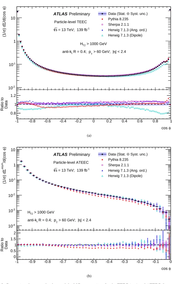
The corrected TEEC and ATEEC distributions are presented and compared to the Monte Carlo predictions

described in Section 3. Figure 2 shows this comparison for the TEEC and ATEEC distributions obtained in

the inclusive H

bin. Additionally, Figure 3 shows this comparison for both the TEEC and ATEEC for

two different regions in H

.

φ cos

-1 -0.8 -0.6 -0.4 -0.2 0 0.2 0.4 0.6 0.8 1

)φ/d(cos Σ) dσ(1/

10-2

10-1

1 10

Syst. unc.)

⊕ Data (Stat.

Pythia 8.235 Sherpa 2.1.1

Herwig 7.1.3 (Ang. ord.) Herwig 7.1.3 (Dipole) Preliminary

ATLAS

= 13 TeV; 139 fb-1

s

Particle-level TEEC

> 1000 GeV HT2

| < 2.4 η > 60 GeV; | R = 0.4; pT

anti-kt

φ cos

-1 -0.8 -0.6 -0.4 -0.2 0 0.2 0.4 0.6 0.8 1

Data Ratio to

0.8 1 1.2

(a)

φ cos

-1 -0.9 -0.8 -0.7 -0.6 -0.5 -0.4 -0.3 -0.2 -0.1 0

)φ/d(cos asym Σ) dσ(1/

10-4

10-3

10-2

10-1

1 10

Syst. unc.)

⊕ Data (Stat.

Pythia 8.235 Sherpa 2.1.1

Herwig 7.1.3 (Ang. ord.) Herwig 7.1.3 (Dipole) Preliminary

ATLAS

= 13 TeV; 139 fb-1

s

Particle-level ATEEC

> 1000 GeV HT2

| < 2.4 η > 60 GeV; | R = 0.4; pT

anti-kt

φ cos

-1 -0.9 -0.8 -0.7 -0.6 -0.5 -0.4 -0.3 -0.2 -0.1 0

Data Ratio to

0 0.5 1 1.5 2

(b)

Figure 2: Comparison between the data and the MC expectations for the TEEC (top) and ATEEC (bottom) for the inclusiveH_T2bin.

φ cos

-1 -0.8 -0.6 -0.4 -0.2 0 0.2 0.4 0.6 0.8 1

)φ/d(cos Σ) dσ(1/

10-2

10-1

1 10

Syst. unc.)

⊕ Data (Stat.

Pythia 8.235 Sherpa 2.1.1 Herwig 7.1.3 (Ang. ord.) Herwig 7.1.3 (Dipole) Preliminary

ATLAS

= 13 TeV; 139 fb-1

s

Particle-level TEEC

< 1400 GeV 1200 GeV < HT2

| < 2.4 η > 60 GeV; | R = 0.4; pT

anti-kt

φ cos -1 -0.8 -0.6 -0.4 -0.2 0 0.2 0.4 0.6 0.8 1

Data Ratio to

0.8 1 1.2

(a)

φ cos

-1 -0.8 -0.6 -0.4 -0.2 0 0.2 0.4 0.6 0.8 1

)φ/d(cos Σ) dσ(1/

10-2

10-1

1 10

Syst. unc.)

⊕ Data (Stat.

Pythia 8.235 Sherpa 2.1.1 Herwig 7.1.3 (Ang. ord.) Herwig 7.1.3 (Dipole) Preliminary

ATLAS

= 13 TeV; 139 fb-1

s

Particle-level TEEC

< 3500 GeV 3000 GeV < HT2

| < 2.4 η > 60 GeV; | R = 0.4; pT

anti-kt

φ cos -1 -0.8 -0.6 -0.4 -0.2 0 0.2 0.4 0.6 0.8 1

Data Ratio to

0.8 1 1.2

(b)

φ cos -1 -0.9 -0.8 -0.7 -0.6 -0.5 -0.4 -0.3 -0.2 -0.1 0 )φ/d(cos asym Σ) dσ(1/

10-4

10-3

10-2

10-1

1 10

Syst. unc.)

⊕ Data (Stat.

Pythia 8.235 Sherpa 2.1.1 Herwig 7.1.3 (Ang. ord.) Herwig 7.1.3 (Dipole) Preliminary

ATLAS

= 13 TeV; 139 fb-1

s

Particle-level ATEEC

< 1400 GeV 1200 GeV < HT2

| < 2.4 η > 60 GeV; | R = 0.4; pT

anti-kt

φ cos -1 -0.9 -0.8 -0.7 -0.6 -0.5 -0.4 -0.3 -0.2 -0.1 0

Data Ratio to

0 0.5 1 1.5

2

(c)

φ cos -1 -0.9 -0.8 -0.7 -0.6 -0.5 -0.4 -0.3 -0.2 -0.1 0 )φ/d(cos asym Σ) dσ(1/

10-4

10-3

10-2

10-1

1 10

Syst. unc.)

⊕ Data (Stat.

Pythia 8.235 Sherpa 2.1.1 Herwig 7.1.3 (Ang. ord.) Herwig 7.1.3 (Dipole) Preliminary

ATLAS

= 13 TeV; 139 fb-1

s

Particle-level ATEEC

< 3500 GeV 3000 GeV < HT2

| < 2.4 η > 60 GeV; | R = 0.4; pT

anti-kt

φ cos -1 -0.9 -0.8 -0.7 -0.6 -0.5 -0.4 -0.3 -0.2 -0.1 0

Data Ratio to

0 0.5 1 1.5

2

(d)

Figure 3: Comparison between the data and the MC expectations for the TEEC (top) and ATEEC (bottom) for two selected regions ofH_T2.

The TEEC and ATEEC distributions presented in Figures 2 and 3 show the usual features observed in the

previous results [46, 47]. The TEEC shows two peaks at cos φ = ± 1 arising from back-to-back config- urations and self correlations, together with a somewhat flat central plateau arising from the wide-angle radiation. The effect of the jet radius R is seen as a kink in the TEEC distributions at cos φ ' 0 . 92. The ATEEC exhibits a steep fall-off of several orders of magnitude between cos φ = − 1 and cos φ = 0.

At low values of H

, the best description of the TEEC distributions is achieved by both Sherpa and Herwig 7 with the angle-ordered parton shower. The dipole parton shower in Herwig 7 does not describe the data well, in particular in the region | cos φ| > 0 . 4, where discrepancies up to 20% are observed close to the edges of the TEEC distribution. Pythia 8 shows discrepancies with data for cos φ ∼ − 0 . 6, where differences of O( 10% ) are observed. A good description of the ATEEC distribution is achieved by both Sherpa and Herwig 7, while Pythia 8 underestimates the height of the higher tail of the distribution and the Herwig 7 sample matched to the dipole parton shower underestimates the values of the ATEEC for cos φ < − 0 . 7.

For large values of H

, Pythia 8 gives the best description of the TEEC data, while both Sherpa and Herwig 7 tend to overestimate the height of the central plateau. The dipole parton shower in Herwig 7 shows a similar behaviour to the low H

region, with the larger discrepancies observed near the edges of the TEEC distribution, although limited to the region | cos φ| > 0 . 7. For the ATEEC, Pythia 8 and Sherpa give a good description of the data, while the Herwig 7 sample matched to the angle-ordered parton shower overestimates the values of the ATEEC for cos φ < − 0 . 7. The cancellation of discrepancies in φ -symmetric regions between the data and the dipole shower in Herwig 7 brings a reasonable agreement for the ATEEC in the high energy regime.

8 Theoretical predictions and uncertainties

The theoretical predictions for the TEEC and ATEEC functions are calculated using pQCD at NLO in powers of the strong coupling constant, α

( µ

) , as implemented in NLOJET++ [42, 43]. The calculations assume n

= 5 massless quark flavours. The value of α

( µ

) which enters in the partonic matrix-element calculation is obtained by evolving the same α

(m

) value provided by the PDF. Jets are reconstructed using the anti- k

algorithm with R = 0 . 4 as implemented in FastJet [79], and the NNLO PDF sets used to convolve the partonic cross sections are provided in the LHAPDF [86] package, namely MMHT 2014 [75], NNPDF 3.0 [87] and CT14 [70]. The azimuthal angular range is restricted in the calculation to

| cos φ| < 0 . 92. This avoids calculating the 2-loop virtual corrections to the 2 → 2 process, as well as suppressing the sensitivity to resolution effects for the angular difference between jet pairs introduced by the jet algorithm.

The renormalisation scale is set for each event to the scalar sum of the transverse momenta of all final-state partons, µ

= H ˆ

[88], while the factorisation scale is set to half this scale, µ

= H ˆ

/ 2 [89].

The pQCD predictions for the TEEC and ATEEC functions obtained using NLOJET++ are calcu-

lated at parton level only. Therefore, in order to compare with the experimental results at particle level, the

predictions are corrected for non-perturbative effects, namely hadronisation and underlying event (UE) by

means of correction factors accounting for these effects. These correction factors are calculated as the ratio

of the MC predictions including both hadronisation and underlying event effects to the MC predictions in

which these effects are not included. The central values for these correction factors have been calculated

using the A14 tune in Pythia 8 [63], and differ from unity in at most 1% in the range | cos φ| < 0 . 92.

Electroweak corrections are not accounted for due to lack of knowledge, although their effect should be similar for three-jet and two-jet production and, thus, cancel to a large extent.

The uncertainties on the theoretical predictions arise from three sources: the scale uncertainties that estimate the contributions of higher-order corrections, the uncertainties on the PDF parameters and the uncertainties on the non-perturbative corrections to the pQCD predictions.

• The scale uncertainties are evaluated by considering independent variations of the renormalisation and factorisation scales by a factor of two, excluding those variations in which µ

and µ

are varied in opposite directions. The uncertainty on the distributions is defined as the envelope of the six resulting variations. The scale uncertainty bands are symmetric for both the TEEC and ATEEC, and their values are below 10% in all regions of the phase space. This is the dominant uncertainty on this analysis.

• The PDF uncertainties are obtained by varying each PDF following the set of eigenvectors / replicas provided by each PDF group [70, 75, 87], and are propagated to the predicted distributions using the corresponding recommendations from each particular PDF set. The resulting uncertainties are below 1% in all regions of the phase space.

• The uncertainties on the non-perturbative corrections are evaluated by considering the envelope of the differences of the 4C [90] and AU2 [91] Pythia 8 tunes with respect to the A14 tune [63].

The value of this uncertainty is below 1% in the phase-space region | cos φ| < 0 . 92, where α

is determined.

9 Determination of the strong coupling constant

The strong coupling constant at the scale of the pole mass of the Z boson, α

(m

) can be determined from the comparison of the data to the theoretical predictions by considering the following χ

function

χ

(α

, λ) ~ = X

bins

(x

− F

(α

, λ)) ~

∆x

+ ∆ ξ

+ X

k

λ

, (1)

where the theoretical predictions are varied according to F

(α

, λ) ~ = ψ

(α

) *

, 1 + X

k

λ

σ

+ -

. (2)

In Equations (1) and (2), α

stands for α

(m

) ; x

is the value of the i -th point of the distribution as measured in data, while ∆x

is its statistical uncertainty. The statistical uncertainty in the theoretical predictions, as well as the uncorrelated modelling uncertainty, are also included as ∆ ξ

, while σ

is the relative value of the k -th correlated source of systematic uncertainty in bin i .

This technique takes into account the correlations between the different sources of systematic uncer-

tainty discussed in Section 6 by introducing the nuisance parameters {λ

} , one for each source of

experimental uncertainty. Thus, the minimum of the χ

function defined in Equation (1) is found in a

149-dimensional space, in which 148 correspond to nuisance parameters {λ

} and one to α

(m

) .

The method also requires an analytical expression for the dependence of each observable on the strong coupling constant, which is given by ψ

(α

) for bin i . For each PDF set, the corresponding α

(m

) variation range is considered and the theoretical prediction is obtained for each value of α

(m

) . The functions ψ

(α

) are then obtained by fitting the predicted values of the TEEC (ATEEC) in each ( H

, cos φ) bin to a second-order polynomial in α

.

For both the TEEC and ATEEC functions, the fits to extract α

(m

) are repeated separately for each H

interval, thus determining a value of α

(m

) for each energy bin. The theoretical uncertainties are determined by shifting the theory distributions by each of the uncertainties separately, recalculating the functions ψ

(α

) and determining a new value of α

(m

). The uncertainty is determined by taking the difference between this value and the nominal one.

Each of the fitted values of α

(m

), which are obtained in the MS subtraction scheme, is then evolved to the corresponding measured scale using the NLO solution to the renormalisation group equation (RGE).

When evolving α

(m

) to α

(Q) , the appropriate matching conditions for the strong coupling constant at the n

= 5 and n

= 6 flavour thresholds are applied so that α

(Q) is a continuous function across quark thresholds.

The values of α

(m

) determined from fits to the TEEC functions, both in the inclusive and ex- clusive H

bins, as well as from the global fit, are presented in Table 2, while the values obtained from fits to the ATEEC functions are presented in Table 3, together with the average Q values, i.e.

the average value of µ

= H ˆ

for each H

bin, and the reduced χ

values at the minimum. The values displayed in Tables 2 and 3 are obtained using the MMHT 2014 PDF in the theoretical predictions.

However, results obtained using CT14 and NNPDF 3.0 agree with these values within the PDF uncertainties.

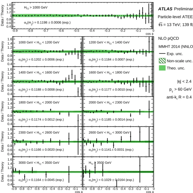
The fitted values of α

(m

) , together with the values of the nuisance parameters, are used to evalu- ate the agreement between the data and the fitted predictions. Figure 4 shows the ratio of the TEEC data to the fitted theoretical distributions for both the inclusive and exclusive bins, together with the theoretical and experimental uncertainties. Similarly, Figure 5 shows the data-to-theory ratios for the ATEEC distributions.

A very good agreement is observed for both the TEEC and ATEEC measurements in all regions of the phase space.

The values of α

(m

) obtained in Tables 2 and 3 are evolved to the corresponding energy scale us-

ing the RGE as explained above. This allows for testing the asymptotic behaviour of QCD by comparing the

measured points with the prediction by the RGE. Figures 6 and 7 show the values of α

(Q) together with the

world average band provided by the Particle Data Group [92] and values of α

obtained in other analyses [46,

47, 93–99]. The results show a good agreement of all measurements with the RGE prediction.

hQi[GeV] α_s(m_Z)value (MMHT 2014) χ²/N_dof Global 0.1196±0.0001 (stat.) ±0.0004 (syst.)^+0.0071_−0.0104(scale)±0.0011 (PDF)±0.0002 (NP) 235.8 / 347 Inclusive 0.1208±0.0002 (stat.) ±0.0006 (syst.)^+0.0081_−0.0101(scale)±0.0009 (PDF)±0.0002 (NP) 42.7 / 91

1219 0.1206±0.0002 (stat.) ±0.0006 (syst.)⁺⁰₋₀^._.⁰⁰⁸³₀₁₀₅(scale)±0.0009 (PDF)±0.0003 (NP) 18.6 / 51 1434 0.1191±0.0003 (stat.) ±0.0007 (syst.)^+0.0080−0.0101(scale)±0.0010 (PDF)±0.0002 (NP) 18.0 / 51 1647 0.1195±0.0002 (stat.) ±0.0007 (syst.)⁺⁰₋₀^._.⁰⁰⁷⁷₀₀₉₄(scale)±0.0011 (PDF)±0.0002 (NP) 38.2 / 51 1856 0.1186±0.0003 (stat.) ±0.0008 (syst.)^+0.0076_−0.0094(scale)±0.0011 (PDF)±0.0004 (NP) 25.9 / 51 2064 0.1183±0.0004 (stat.) ±0.0010 (syst.)⁺⁰₋₀^._.⁰⁰⁷¹₀₀₈₄(scale)±0.0012 (PDF)±0.0005 (NP) 22.4 / 27 2300 0.1192±0.0004 (stat.) ±0.0011 (syst.)^+0.0066_−0.0075(scale)±0.0012 (PDF)±0.0004 (NP) 21.3 / 27 2636 0.1185±0.0004 (stat.) ±0.0012 (syst.)⁺⁰₋₀^._.⁰⁰⁶⁴₀₀₇₂(scale)±0.0012 (PDF)±0.0001 (NP) 22.0 / 27 2952 0.1179±0.0005 (stat.) ±0.0014 (syst.)^+0.0059_−0.0064(scale)±0.0013 (PDF)±0.0003 (NP) 25.0 / 27 3383 0.1194±0.0007 (stat.) ±0.0014 (syst.)^+0.0052−0.0052(scale)±0.0013 (PDF)±0.0002 (NP) 15.3 / 13 4095 0.1167±0.0010 (stat.) ±0.0014 (syst.)⁺⁰₋₀^._.⁰⁰⁵⁰₀₀₅₃(scale)±0.0015 (PDF)±0.0003 (NP) 13.5 / 13 Table 2: Values of the strong coupling constant at the Z boson mass scale,α_s(m_Z), obtained from fits to the TEEC function using MMHT 2014 parton distribution functions. The values of the average interaction scalehQiare shown in the first column, while the values of the χ²function at the minimum are shown in the third column. The uncertainty referred to as NP is the one related to the non-pQCD corrections.

hQi[GeV] α_s(m_Z)value (MMHT 2014) χ²/N_dof

Global 0.1195±0.0002 (stat.) ±0.0006 (syst.)⁺⁰₋₀^._.⁰⁰⁸⁴₀₁₀₆(scale)±0.0009 (PDF)±0.0003 (NP) 254.1 / 173 Inclusive 0.1198±0.0002 (stat.) ±0.0006 (syst.)⁺⁰₋₀^._.⁰⁰⁷⁸₀₀₉₅(scale)±0.0010 (PDF)±0.0002 (NP) 46.3 / 45

1219 0.1202±0.0003 (stat.) ±0.0006 (syst.)^+0.0079−0.0098(scale)±0.0010 (PDF)±0.0002 (NP) 25.7 / 25 1434 0.1184±0.0003 (stat.) ±0.0007 (syst.)⁺⁰_−0.0098^.0078(scale)±0.0011 (PDF)±0.0002 (NP) 35.6 / 25 1647 0.1188±0.0004 (stat.) ±0.0007 (syst.)^+0.0073−0.0087(scale)±0.0012 (PDF)±0.0001 (NP) 41.9 / 25 1856 0.1177±0.0006 (stat.) ±0.0008 (syst.)⁺⁰₋₀^._.⁰⁰⁷²₀₀₈₃(scale)±0.0013 (PDF)±0.0006 (NP) 24.6 / 25 2064 0.1174±0.0008 (stat.) ±0.0009 (syst.)^+0.0069_−0.0078(scale)±0.0013 (PDF)±0.0007 (NP) 18.7 / 13 2300 0.1185±0.0009 (stat.) ±0.0010 (syst.)⁺⁰₋₀^._.⁰⁰⁶³₀₀₆₇(scale)±0.0014 (PDF)±0.0005 (NP) 22.5 / 13 2636 0.1166±0.0016 (stat.) ±0.0012 (syst.)^+0.0062_−0.0066(scale)±0.0015 (PDF)±0.0000 (NP) 21.7 / 13 2952 0.1141±0.0029 (stat.) ±0.0013 (syst.)⁺⁰−0^..⁰⁰⁶²0069(scale)±0.0018 (PDF)±0.0003 (NP) 15.2 / 13 3383 0.1164±0.0043 (stat.) ±0.0015 (syst.)^+0.0050_−0.0044(scale)±0.0017 (PDF)±0.0001 (NP) 6.3 / 6 4095 0.1029±0.0163 (stat.) ±0.0014 (syst.)^+0.0066−0.0012(scale)±0.0010 (PDF)±0.0003 (NP) 5.9 / 6 Table 3: Values of the strong coupling constant at the Z boson mass scale,α_s(m_Z), obtained from fits to the ATEEC function using MMHT 2014 parton distribution functions. The values of the average interaction scalehQiare shown in the first column, while the values of the χ²function at the minimum are shown in the third column. The uncertainty referred to as NP is the one related to the non-pQCD corrections.

φ cos

-0.8 -0.6 -0.4 -0.2 0 0.2 0.4 0.6 0.8

Data / Theory _0.8 0.9 1 1.1

1.2 H_T2 > 1000 GeV

0.0007 (exp.)

± ) = 0.1208 (mZ

αs

cos φ

-0.8 -0.6 -0.4 -0.2 0 0.2 0.4 0.6 0.8

Data / Theory

0.8 0.9 1 1.1

1.2 1000 GeV < H_T2 < 1200 GeV

0.0006 (exp.)

± ) = 0.1206 (mZ

αs

cos φ

-0.8 -0.6 -0.4 -0.2 0 0.2 0.4 0.6 0.8

Data / Theory

0.8 0.9 1 1.1 1.2

< 1400 GeV 1200 GeV < HT2

0.0007 (exp.)

± ) = 0.1191 (mZ

αs

φ cos

-0.8 -0.6 -0.4 -0.2 0 0.2 0.4 0.6 0.8

Data / Theory

0.8 0.9 1 1.1

1.2 1400 GeV < H_T2 < 1600 GeV

0.0007 (exp.)

± ) = 0.1195 (mZ

αs

φ cos

-0.8 -0.6 -0.4 -0.2 0 0.2 0.4 0.6 0.8

Data / Theory

0.8 0.9 1 1.1 1.2

< 1800 GeV 1600 GeV < HT2

0.0009 (exp.)

± ) = 0.1186 (mZ

αs

cos φ

-0.8 -0.6 -0.4 -0.2 0 0.2 0.4 0.6 0.8

Data / Theory

0.8 0.9 1 1.1

1.2 1800 GeV < H_T2 < 2000 GeV

0.0011 (exp.)

± ) = 0.1183 (mZ

αs

cos φ

-0.8 -0.6 -0.4 -0.2 0 0.2 0.4 0.6 0.8

Data / Theory

0.8 0.9 1 1.1 1.2

< 2300 GeV 2000 GeV < HT2

0.0011 (exp.)

± ) = 0.1192 (mZ

αs

φ cos

-0.8 -0.6 -0.4 -0.2 0 0.2 0.4 0.6 0.8

Data / Theory

0.8 0.9 1 1.1

1.2 2300 GeV < H_T2 < 2600 GeV

0.0013 (exp.)

± ) = 0.1185 (mZ

αs

φ cos

-0.8 -0.6 -0.4 -0.2 0 0.2 0.4 0.6 0.8

Data / Theory

0.8 0.9 1 1.1 1.2

< 3000 GeV 2600 GeV < HT2

0.0015 (exp.)

± ) = 0.1179 (mZ

αs

φ cos -0.8 -0.6 -0.4 -0.2 0 0.2 0.4 0.6 0.8

Data / Theory

0.8 0.9 1 1.1

1.2 3000 GeV < H_T2 < 3500 GeV

0.0015 (exp.)

± ) = 0.1194 (mZ

αs

φ cos -0.8 -0.6 -0.4 -0.2 0 0.2 0.4 0.6 0.8

Data / Theory

0.8 0.9 1 1.1 1.2

> 3500 GeV HT2

0.0017 (exp.)

± ) = 0.1167 (mZ

αs

Preliminary ATLAS

Particle-level TEEC = 13 TeV; 139 fb-1

s

NLO pQCD

MMHT 2014 (NNLO) Exp. unc.

Non-scale unc.

Theo. unc.

R = 0.4 anti-kt

> 60 GeV pT

| < 2.4 η

|

Figure 4: Ratios of the data to the fitted theoretical predictions for the TEEC measurements in inclusive and exclusive H_T2bins. The green band shows the theoretical uncertainties, dominated by the scale variations, while the error bars show the experimental uncertainties, where correlations between the fit parameters have been taken into account.

φ cos

-0.9 -0.8 -0.7 -0.6 -0.5 -0.4 -0.3 -0.2 -0.1 0

Data / Theory _0.4^0.6 0.8 1 1.2 1.4

1.6 H_T2 > 1000 GeV

0.0006 (exp.)

± ) = 0.1198 (mZ

αs

cos φ

-0.9 -0.8 -0.7 -0.6 -0.5 -0.4 -0.3 -0.2 -0.1 0

Data / Theory

0.4 0.6 0.8 1 1.2 1.4 1.6

< 1200 GeV 1000 GeV < HT2

0.0006 (exp.)

± ) = 0.1202 (mZ

αs

cos φ

-0.9 -0.8 -0.7 -0.6 -0.5 -0.4 -0.3 -0.2 -0.1 0

Data / Theory

0.4 0.6 0.8 1 1.2 1.4 1.6

< 1400 GeV 1200 GeV < HT2

0.0007 (exp.)

± ) = 0.1184 (mZ

αs

φ cos

-0.9 -0.8 -0.7 -0.6 -0.5 -0.4 -0.3 -0.2 -0.1 0

Data / Theory

0.4 0.6 0.8 1 1.2 1.4 1.6

< 1600 GeV 1400 GeV < HT2

0.0008 (exp.)

± ) = 0.1188 (mZ

αs

φ cos

-0.9 -0.8 -0.7 -0.6 -0.5 -0.4 -0.3 -0.2 -0.1 0

Data / Theory

0.4 0.6 0.8 1 1.2 1.4 1.6

< 1800 GeV 1600 GeV < HT2

0.0010 (exp.)

± ) = 0.1177 (mZ

αs

cos φ

-0.9 -0.8 -0.7 -0.6 -0.5 -0.4 -0.3 -0.2 -0.1 0

Data / Theory

0.4 0.6 0.8 1 1.2 1.4 1.6

< 2000 GeV 1800 GeV < HT2

0.0012 (exp.)

± ) = 0.1174 (mZ

αs

cos φ

-0.9 -0.8 -0.7 -0.6 -0.5 -0.4 -0.3 -0.2 -0.1 0

Data / Theory

0.4 0.6 0.8 1 1.2 1.4 1.6

< 2300 GeV 2000 GeV < HT2

0.0014 (exp.)

± ) = 0.1185 (mZ

αs

φ cos

-0.9 -0.8 -0.7 -0.6 -0.5 -0.4 -0.3 -0.2 -0.1 0

Data / Theory

0.4 0.6 0.8 1 1.2 1.4 1.6

< 2600 GeV 2300 GeV < HT2

0.0020 (exp.)

± ) = 0.1166 (mZ

αs

φ cos

-0.9 -0.8 -0.7 -0.6 -0.5 -0.4 -0.3 -0.2 -0.1 0

Data / Theory

0.4 0.6 0.8 1 1.2 1.4 1.6

< 3000 GeV 2600 GeV < HT2

0.0031 (exp.)

± ) = 0.1141 (mZ

αs

φ cos -0.9 -0.8 -0.7 -0.6 -0.5 -0.4 -0.3 -0.2 -0.1 0

Data / Theory

0.4 0.6 0.8 1 1.2 1.4 1.6

< 3500 GeV 3000 GeV < HT2

0.0045 (exp.)

± ) = 0.1164 (mZ

αs

φ cos -0.9 -0.8 -0.7 -0.6 -0.5 -0.4 -0.3 -0.2 -0.1 0

Data / Theory

0.4 0.6 0.8 1 1.2 1.4 1.6

> 3500 GeV HT2

0.0164 (exp.)

± ) = 0.1029 (mZ

αs

Preliminary ATLAS

Particle-level ATEEC = 13 TeV; 139 fb-1

s

NLO pQCD

MMHT 2014 (NNLO) Exp. unc.

Non-scale unc.

Theo. unc.

R = 0.4 anti-kt

> 60 GeV pT

| < 2.4 η

|

Figure 5: Ratios of the data to the fitted theoretical predictions for the ATEEC measurements in inclusive and exclusiveH_T2bins. The green band shows the theoretical uncertainties, dominated by the scale variations, while the error bars show the experimental uncertainties, where correlations between the fit parameters have been taken into account.