Quantum time mirrors Phillipp Reck

Phillipp Reck

¹

, Cosimo Gorini

¹

, Arseni Goussev

²

, Viktor Krueckl

¹

, Mathias Fink

³

, Klaus Richter

^1∗

1

Institut f¨ ur Theoretische Physik, Universit¨ at Regensburg, 93040 Regensburg, Germany

2

Department of Mathematics and Information Sciences,

Northumbria University, Newcastle upon Tyne, NE1 8ST, United Kingdom and

3

Institut Langevin, ESPCI, CNRS, PSL Research University, 1 rue Jussieu, 75005, Paris, France (Dated: March 25, 2016)

Both metaphysical and practical considerations related to time inversion have intrigued scientists for generations. Physicists have strived to devise and implement time-inversion protocols, in partic- ular different forms of “time mirrors” for classical waves. Here we propose two conceptually different realisations of instantaneous time mirrors for quantum systems, i.e. controlled time discontinuities acting through pulses on wavefronts and leading to distinct wave function echoes with high fidelities.

The first concept exploits up to now unrelated mechanisms of wavefront time inversion and popu- lation reversal in spatially extended two-level systems, the latter quintessential to spin echoes. It can be implemented in Dirac-like systems, such as (real or artificial) graphene. The second protocol is based on a non-linear mirror for a Bose-Einstein condensate whose dynamics is described by the non-linear Schr¨ odinger equation, and is realisable in cold atom setups.

∗To whom correspondence should be addressed. E-mail: klaus.richter@ur.de

arXiv:1603.07503v1 [cond-mat.mes-hall] 24 Mar 2016

simultaneously flip the spins, which effectively evolve “back in time” regaining (“echoing”) the initially aligned, phase coherent configuration.

Another successful approach to time inversion has been developed for classical waves based on time-reversal mirrors implemented with acoustic [5, 6], elastic [7], electromagnetic [8] and recently water waves [9, 10]. It relies on the fact that any wave field can be completely determined in a volume by knowing only the field at any enclosing surface (a spatial boundary). It requires the use of receiver-emitter antennas positioned on the surface that record an incident wavefront and later rebroadcast a t-inverted copy of the signal. If an initially localised pulse, e.g. a wave emitted from any source, is left to evolve for a certain time and then in this manner t-inverted on a boundary, it can trace its way back to the initial source and there refocus or “echo” [11, 12]. Note that this process is difficult to implement in optics because of the lack of controllable antennas [13], and the standard solution to create time-reversed waves is to work with monochromatic light and use non-linear regimes such as three-wave or four-wave mixing [14, 15].

A potent alternative to wave field control via spatial boundaries is the manipulation of time boundaries [16–22].

Explicit time reversal protocols for one-dimensional (1D) propagation were proposed for the kicked rotator model of atomic matter waves [23] and for electromagnetic waves [24, 25], the latter based on time- and space-modulated perturbations of a photonic crystal with linear dispersion. The latest development in this context is the concept of an instantaneous time mirror, which has been verified experimentally [26] in the field of gravity-capillary waves. A sudden modification of water wave celerity obtained from a vertical acceleration of a bath of water creates a time-reversed wave. This time disruption realises an instantaneous time mirror in the entire space. Such a mirror can be viewed as the analogue in time to a standard mirror that acts on space.

In view of these various successful concepts for time reversal of classical wave fields there remains the long-standing challenge to devise t-inversion protocols for quantum wave functions. In other words, are Quantum Time Mirrors (QTMs) feasible for spatially extended quantum waves, beyond the Hahn echo for spin? A direct adaption of the aforementioned classical wave strategies appears difficult: On the one hand, recording and properly re-emitting waves would require to measure and thereby massively change the quantum state; on the other hand, the intriguing concept of a time mirror for water waves cannot be directly transferred to wave functions due to the inherently different structure of the underlying differential equations: the classical wave equation and Schr¨ odinger equation.

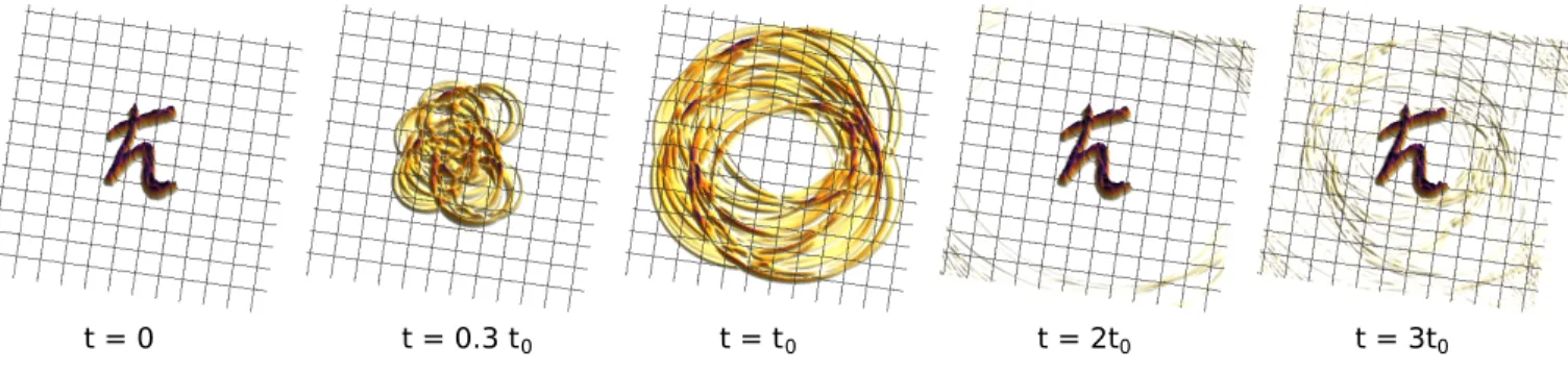
Here we show that, still, it is indeed possible to devise (instantaneous) QTMs for the time evolution of wave functions. We propose two concepts of QTMs based on completely different physical principles. The first QTM concerns a (bosonic or fermionic) Dirac-like system, such as graphene, and is based on the “population reversal”

principle at the heart of spin echoes. As such, this approach unifies two up to now distinct paradigms, the t-inversion of a spatially extended wave and the generation of a (pseudo)spin echo. Fig.1 gives a taste of its effectiveness: an initially ~ -shaped wave packet evolves in time progressively losing its profile, until the action of the instantaneous QTM, a short pulse at t = t

0

apparently inverts the propagation and leads to a distinct echo at t = 2t

0

; the subsequent echo at t = 3t

0

is due to a further QTM pulse at t = 2.5t

0

.

The second QTM we propose is non-linear, acting on a Bose-Einstein condensate cloud whose dynamics is described by the non-linear Schr¨ odinger equation. In both settings almost perfect wave function echoes can be generated, and we discuss the appropriate parameter ranges for this to happen. In particular, lithium Bose-Einstein condensates appear perfectly suited for the implementation of the non-linear QTM.

II. RESULTS

A. Quantum Time Mirror for graphene-like systems

Let us start by considering a two-dimensional (2D) Dirac-Weyl system. This could describe fermions in real[27] and

artificial[28] graphene, surface states of topological insulators[29], Dirac plasmons in metallic nanoparticle lattices[30],

polaritons in a honeycomb lattice[31] and possibly eigenmodes of acoustic graphene[32] near the K-points. In such

a system the velocity is constant – it does not depend on the k-vector – and equal in magnitude, but opposite in

direction on the upper and lower Dirac cones. Our t-inversion protocol aims at inducing a “population reversal”,

FIG. 1. Echo in a Dirac-Weyl quantum system. An ~ -shaped wave packet (at t = 0) becomes completely blurred when propagating until t = t

0

. A fast quantum time reversal pulse at t = t

0

leads to a nearly perfect echo at t = 2t

0

. The last panel (at t = 3t

0

) shows a second echo after a further subsequent pulse at t = 2.5t

0

.

say from the upper to the lower Dirac cone, which corresponds to an inversion of the velocity and thus effectively a propagation back in time. This can be achieved by applying a short, spatially uniform perturbation opening a gap in the spectrum: Once initial upper cone states suddenly find themselves in the forbidden gap region, they start Rabi-like oscillations between the upper and lower branches of the spectrum (corresponding to Zitterbewegung in the Dirac equation for particles and holes). A proper tuning of such oscillations ensures that, by the time the perturbation is switched off and the gap closes, the states will end up in the lower Dirac cone. This process requires a non-adiabatic perturbation as quantified below.

The effective Dirac Hamiltonian reads

H = ak · σ + M (t)σ

z

= H

0

+ H

1

, M (t) =

M

0

, t

0

< t < t

0

+ ∆t,

0, otherwise, (1)

where (the mass term) M (t) acts as the time-dependent perturbation which temporarily opens a gap. The eigenener- gies and eigenstates of H

0

are E

_±

= ±ak and ψ

_±

(k) =

^√1

2

1

±e

^iθk

, with θ

k

the polar angle in k-space. During the pulse the eigenenergies of H are ε

±

= M

0

± q

M

₀²

+ E

_±²

. In the time interval ∆t, an initial H

0

eigenstate is subject to Rabi-like oscillations, whose cycle depends on the pulse strength M

0

and length ∆t. The amplitude A to end up in the counter-propagating H

0

eigenstate at t = t

0

+ ∆t after the pulse can be tuned by adjusting both parameters.

A straightforward calculation yields (see Supplementary Note 1) A(k) = hψ

±,k

| e

^−~iH∆t

| ψ

∓,k

i

= − i

p 1 + η

²

sin µ p

1 + η

²

, (2)

where we introduced the dimensionless parameters η = ak/M

₀

and µ = M

₀

∆t/ ~ . The amplitude needs to be maximised for optimal echo strength, which then requires η 1, µ ≈ π(n + 1/2), n ∈ Z , corresponding to ak M

0

≈ π ~ /2∆t for n = 0. In general, given an initial wave packet ψ(r, 0) = (2π)

⁻²

R

d

²

kψ(k, 0)e

^ik·r

, a convenient measure of the echo strength is given by the correlation

C(t) = Z

d

²

r |ψ(r, 0)||ψ(r, t)| (3) between the moduli of the amplitudes at times 0 and t.

To illustrate the QTM effect, a complicated wave packet resembling ~ is numerically propagated in time (see Fig.

1) by a wave packet propagation algorithm (see Methods). At times t

0

and 2.5t

0

, a pulse with M

0

= 8hE

k

i and

µ = M

0

∆t/ ~ = π/2 is applied, with ∆t t

0

. Here hE

k

i = ahki is the mean wave packet energy, i.e. hηi = 1/8. The

snapshots in Fig. 1 demonstrate that even after full destruction the spatial distribution of the initial wave packet can

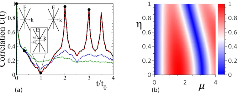
be reconstructed. This is quantified and confirmed in Fig. 2a), showing the corresponding correlation (3). At the echo

time (t = 2t

0

+ ∆t ≈ 2t

0

), major parts of the time propagated wave packet indeed return to the initial position. Our

QTM mechanism is not limited to a single pulse: subsequent kicks at t = 2.5t

0

and t = 3.25t

0

cause further peaks,

albeit of decreasing size.

FIG. 2. Quantitative analysis of the echo strength. (a) Correlation C(t), equation (3), obtained from numerical propagation of the ~ -wave, see Fig. 1. Black circles mark the snapshot times. The solid black curve shows distinct echo peaks for the clean Dirac system, equation(1). The insets show sketches of the Dirac-type dispersion with a gap opening at t = t

0

. Further curves correspond to different disorder types: gap disorder with τ

gap

≈ 0.2t

0

(red dotted), spatial disorder with τ

imp

≈ 0.8t

0

(blue) and τ

imp

≈ 0.2t

0

(green). τ

imp

and τ

gap

are the respective elastic scattering times (see text and Supplementary Note 2). (b) Modulus |A(k)| of the transition amplitude, equation (2), plotted as a function of η and µ.

The distinct echo peaks are based on the linear dispersion relation, implying no wave packet spreading and a k- independent absolute value of the velocity (see Supplementary Note 1). Furthermore the kinetic phases accumulated by each k-mode during forward (0 → t

0

) and backward (t

0

+ ∆t → 2t

0

+ ∆t) propagation add up to zero.

For an arbitrary wave packet, the echo strength C(2t

0

+ ∆t) is analytically given solely in terms of the amplitude A(k) and the wave packet at t = 0 as

C(2t

₀

+ ∆t) = Z

d

²

r ψ(r, 0)

Z d

²

k

(2π)

²

A(k)ψ(k, 0)e

^ik·r

. (4) Figure 2b) shows the η- and µ-dependence of |A(k)|, obtained from the time-reversal amplitude (2). One finds extended stripes of high fidelity. To check this analytical result we simulate the propagation of a normalised 2D Gaussian wave packet with positive energy and small k-space width ∆k k

₀

compared to the mean absolute value k

₀

of its wave vector, such that A(k) ≈ A(k

₀

) for all k-modes involved. Under these assumptions, equation (4) reduces to C(2t

0

+ ∆t) ≈ |A(k

0

)| (see Supplementary Note 1), which can be compared with the correlation C(2t

0

+ ∆t), equation (3), obtained from full numerical time evolution. As the mean difference between analytics and numerics is 0.03, only the analytical plot is shown.

Let us now investigate the QTM robustness to disorder, typically present in a real system. For the sake of clarity

we keep the discussion at a qualitative level, and refer to Supplementary Note 2, for quantitative details. We consider

two types of disorder: a static spatial disorder potential, as well as a spatially random pulse strength (referred

to as “gap disorder”). Spatial disorder enters into the Hamiltonian (1) as a time- and (pseudo)spin-independent

potential V

_imp

(r)σ

₀

, where σ

₀

is the unit matrix in (pseudo)spin-space. Gap disorder is instead given by V

_gap

(r)σ

_z

for

t ∈ [t

₀

, t

₀

+ ∆t], i.e. only during the pulse. Both random potentials are Gaussian distributed with width U

_imp

or U

_gap

.

Clearly, the echo is more sensitive to a static random impurity potential than to gap disorder (see Fig. 2a). This is

expected, and can be understood within the framework of Loschmidt echo theory [12, 33, 34]: If a t-inversion protocol

is not perfect, the echo signal decays as a function of the propagation time t

0

. Spatial disorder reduces the fidelity,

since the QTM mechanism, even for an optimally calibrated pulse, achieves “population reversal” without directly

affecting the impurity scattering dynamics. In other words, the protocol does not involve V

_imp

(r) → −V

imp

(r). Gap

disorder plays in principle a similar QTM-breaking role. However, and contrary to spatial disorder, it is active only

during the very short pulse duration time ∆t t

0

and thus causes only negligible echo losses, reflected in the prefect

agreement of the black line and dotted red line in Fig. 2a).

B. Quantum Time Mirror for Bose-Einstein condensate clouds

As a second complementary quantum system that enables quantum time mirroring we consider a Bose-Einstein condensate cloud moving in D dimensions, with interatomic interactions turned on only during a short time interval.

The wave function Ψ(r, t) of the atomic cloud evolves, starting from an initial state Ψ

0

(r) = Ψ(r, 0), in accordance with the non-linear Schr¨ odinger equation i ~

^∂Ψ_∂t

= −

_2m^~2

∇

²

Ψ+ λf(t−t

0

)|Ψ|

²

Ψ. Here, m is the atomic mass, λ quantifies the nonlinearity strength, and t

0

denotes the time around which the non-linear term representing interaction effects is switched on. The function f (ζ) is sharply peaked around ζ = 0 and is chosen to satisfy the normalisation condition R

+∞

−∞

dζf (ζ) = 1. We take f to be a δ-function in our analytical calculations and a Gaussian peak f (ζ) =

^{√ 1}

2π∆t

e

^{− ζ}

2 2∆t2

in all numerical simulations. The pulse length ∆t t

0

is 0.001t

0

and 0.0025t

0

in one and two dimensions, respectively.

Wave packet dynamics in the presence of an infinitesimally short non-linear kick, f (ζ) = δ(ζ), can be described as follows. Rescaling t → t

0

t, r → q

~t0

m

r, Ψ →

m

~t₀

^D/4

Ψ, and λ → ~

^~_m^t0

^D/2

λ, we write the non-linear Schr¨ odinger equation in a dimensionless form as

i ∂Ψ

∂t = − 1

2 ∇

²

Ψ + λδ(t − 1)|Ψ|

²

Ψ . (5)

The evolution of the wave function from Ψ

₀

(r) at t = 0 to its value Ψ

₋

(r) = Ψ(r, t = 1

⁻

) right before the kick is given by

Ψ

₋

(r) = Z

d

^D

r

⁰

K(r − r

⁰

, t)Ψ

₀

(r

⁰

) , (6) where the integration runs over the infinite D-dimensional space, and K(q, t) = (2πit)

^−D/2

exp [i|q|

²

/(2t)] is the free- particle propagator. The non-linear kick results in an instantaneous change of the wave function from Ψ

₋

(r) at t = 1

⁻

to

Ψ

+

(r) = Ψ

₋

(r)e

^{−iλ|Ψ−(r)|2}

(7)

at t = 1

⁺

. Indeed, during the time interval 1

⁻

< t < 1

⁺

, the wave function transformation is dominated by the second term in the right-hand side of equation (5), and effectively governed by the differential equation

^{∂ln Ψ(r,t)}_∂t

=

−iλ|Ψ

₋

(r)|

²

δ(t − 1), the solution of which is given by equation (7). After the kick, the wave function evolves freely, so that Ψ(r, t) = R

d

^D

r

⁰

K(r − r

⁰

, t)Ψ

₊

(r

⁰

) for all times t > 1.

As evident from equation (7), the instantaneous non-linear kick alters the phase of the wave function without producing any probability density redistribution, so that ρ(r) ≡ |Ψ

+

(r)|

²

= |Ψ

₋

(r)|

²

. The phase change however affects the probability current, whose dimensionless expression reads j(r, t) = Im

Ψ

^∗

(r, t)∇Ψ(r, t)

. A straightforward evaluation of the current right after the kick, j

₊

= Im

Ψ

^∗₊

∇Ψ

+

, yields

j

₊

= j

₋

+ ∆j with ∆j = −λρ∇ρ , (8) where j

₋

= Im

Ψ

^∗₋

∇Ψ

−

is the probability current immediately preceding the kick. This in turn means that, by properly tuning the kicking strength λ, the wave propagation direction can be reversed for those parts of the matter wave for which the vector ∇ρ is aligned (or anti-aligned) with j

₋

. Below we show that in geometries accessible in atom-optics experiments this reversal effect is robust and well-pronounced.

As our first example, we consider the case of the initial state given by a 1D Gaussian wave packet, Ψ

0

(x) = (πσ

²

)

^−1/4

exp

− x

²

2σ

²

+ ikx

, (9)

characterised by the dimensionless real spatial dispersion σ and average momentum k. The corresponding wave function at time t = 1

⁻

is obtained from equation (6) and reads (up to a position-independent phase factor) Ψ

−

(x) = [π(σ

²

+ σ

⁻²

)]

^−1/4

exp[−ξ

²

/2(σ

²

+ i) + ikξ] with ξ = x − k denoting the distance from the wave packet center. Thus, the probability density at t = 1 is ρ = exp(−ξ

²

/σ

²₁

)/ √

πσ

1

, where σ

1

= √

σ

²

+ σ

⁻²

is the dispersion of the wave packet at the time of the kick. The probability currents before and after the kick are, respectively, j

₋

=

k +

_σ2^ξ_σ2 1

ρ and j

₊

= j

₋

+ ∆j, with ∆j =

^2λξ_σ2

1

ρ

²

. The minimal kick strength λ

_min

necessary for reversing the direction of motion of (and effectively reflecting) a part of the wave packet can be estimated by requiring j

+

= 0 at ξ = −σ

1

. In the case of a fast moving wave packet, such that k 1/σ

²

σ

1

, this estimation yields

λ

min

' Ck

σ

²

+ 1 σ

²

(10)

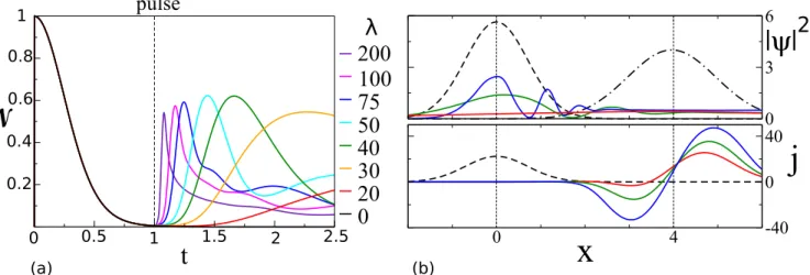
FIG. 3. Echo of a 1D Gaussian wave packet subjected to a short, non-linear pulse. All quantities are dimensionless according to the rescaling in the text. (a) Norm correlation, equation (12), as a function of time for various pulse strengths λ of a kick at t = 1 at fixed wave packet width σ = 1 and momentum k = 4, yielding echoes up to 60%. (b) Upper panel: real space probability density ρ = |ψ|

²

at t = 0 (black dashed curve), t = 0.99 (just before pulse, black dashed-dotted curve), and at the peak echo times (coloured curves, colour code as in (a)). Notice that the latter depend on λ, as evident from (a). Lower panel:

current density j at t = 0 (black dashed curve) and t = 1.01 (right after the pulse, colour code as in (a)). A negative current density indicates the part of the wave packet reverses its propagation direction thereby causing the echo. The minimal kicking strength for the used parameters, as predicted by equation (10), is λ

min

' 20 (red curve); the associated negative current density is not sufficient for echo generation.

with C = e √

π/2 ' 2.4. Then, given a kicking strength λ > λ

min

, the time t

echo

at which the reflected part of the wave packet reaches its initial position, leading to a partial echo of the original wave packet, can be evaluated as follows. The velocity of the reflected wave is k

_rev

' j

₊

_ξ=−σ

1

' k −

_Cσ^λ2 1

= 1 −

_λ^λ

min

k, and the revival occurs when

|k

rev

|(t

echo

− 1) = k or, correspondingly, at

t

echo

= λ λ − λ

min

. (11)

The numerical calculations are based on the same wave packet propagation code employed in Sec. II A. The echo strength is quantified by the norm correlation between the initial and the time propagated wave packet defined as [35]

N (t) =

R d

^D

r |Ψ

0

(r)|

²

|Ψ(r, t)|

²

q R

d

^D

r |Ψ

0

(r)|

⁴

R

d

^D

r |Ψ(r, t)|

⁴

. (12)

Figure 3a) presents N (t) for various pulse strengths λ at constant σ and k, demonstrating echo strengths up to 60%.

The occurring lower peaks at higher λ for larger times are due secondary peaks of the distorted wave packet, which can be seen in Fig. 3b): This panel shows the spatial probability density ρ = |ψ|

²

at times t = 0 (black dashed curve) and t = 0.99 (immediately before pulse, black dashed-dotted curve), as well as the reflected wave packets for different λ’s (colour code as in panel (a)), each shown at its peak echo time. In the lower plot, the current density j is shown directly after the pulse t = 1.01. Parts of the wave packet with negative current density move backwards leading to the echo. For the parameters used, the estimated value for the minimal pulse strength in (10) is λ

_min

' 20 corresponding to the red curve, whose current density exhibits only a vanishing negative part that is insufficient for echo generation, thus verifying the prediction (10).

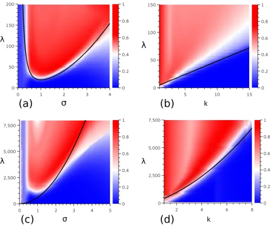
To explore the parameter space for the possibility of achieving echoes, the peak of the norm correlation (in time) is plotted as a function of λ and σ in Fig. 4a) and as a function of λ and k in Fig. 4b). The black curve shows the analytic approximation (10) of the minimal pulse strength λ

_min

. Although it does not fit perfectly, the analytic approximation is in good agreement and still well-suited to approximate the minimal pulse strength required for a time-reversal.

We further investigate the dynamics of a 2D wave packet, initially given by Ψ

0

(r) =

r 1

2π

^3/2

Rσ exp

− (r − R)

²

2σ

²

+ ikr

(13)

FIG. 4. Parameter space for echoes in the non-linear quantum 1D system (a-b) and a 2D system (c-d). All quantities are dimensionless according to the rescaling in the text. The echo peak of the norm correlation (12) is plotted as a function of λ and σ ((a) and (c)) and as a function of λ and k ((b) and (d)). The constant parameters are (a) k = 4, (b) σ = 1, (c) k = 4 and (d) σ = 2. In the 2D case of Gaussian ring (c-d), the radius is chosen to be R = 6. The black curves are the analytical approximations (equation (10) in 1D and by (14) in 2D) for the minimal pulse strength λ

min

required to generate an echo.

with r = |r| and k > 0. For R σ, the wave function is normalised to one and describes a Gaussian ring of radius R and width σ that spreads radially with the average velocity k. A straightforward (although tedious; see Supplementary Note 3) calculation shows that, in the parametric regime defined by 1 σ R and kR 1, the wave packet at t = 1

⁻

has the form (up to a spatially uniform phase) Ψ

₋

(r) = (2π

^3/2

R

₁

σ)

^−1/2

exp[−(r − R

₁

)

²

/2σ

²

+ ikr], where R

₁

= R + k is the radius of the Gaussian ring at time 1

⁻

. Thus, the corresponding probability density is given by ρ = (2π

^3/2

R

1

σ)

⁻¹

exp[−(r − R

1

)

²

/σ

²

], and the probability current at t = 1

⁺

, reads j

+

=

kρ +

^2λ(r−R_σ2 ¹⁾

ρ

²

r r

. Then, the evaluation of the minimal kick strength required to trigger a probability density echo proceeds in close analogy with the corresponding 1D calculation, resulting in

λ

_min

' 2πC(R + k)kσ

²

. (14)

Finally, just as in the 1D case, the echo time is determined by equation (11).

The numerical calculations (Fig. 4c and d) attest the possibility of pronounced echoes also in the 2D setup.

Although the parameter range is not in the regime of the analytical approximation, the value of λ

_min

in equation (14) is still well-suited to estimate the minimal pulse strength λ required (see black curves).

The colour plots in Fig. 4 seem to imply λ > λ

min

(marked as black lines) to be the only echo requirement for echo generation. However for large λ the wave packet splits into many peaks, as shown in Fig. 3b), blue curve for λ = 200. In such a scenario the norm correlation is still fairly high, but the wave packet might not longer have the desired shape. The effect of many peaks, i.e. very large λ, on the norm correlation can be seen in Fig. 4c), where the echo strength moderately declines for σ ≈ 1 and λ > 3000.

III. DISCUSSION

The analytical and numerical considerations presented in this work confirm the principles behind both QTMs.

In the case of QTM for pseudo-relativistic graphene-like systems, this means that a sufficiently fast and spatially

are quantum counterparts of the instantaneous time mirror for water waves very recently realised by V. Bacot et al.

[26], however relying on a different set of principles.

Various experimental realisations of the QTMs proposed here can be imagined. For Dirac systems our QTM represents a general proof of concept, based on a single-particle picture and including the assumption that the inelastic relaxation time of the injected wave packet is larger than t

0

. This condition might still be restrictive in real graphene [36–38], suggesting that some form of articifial graphene [28, 31] could be rather amenable to a straightforward experimental implementation of the QTM. On the other hand we demonstrated that the t-inversion protocol is fairly robust to elastic disorder and practically insensitive to pulse (gap) disorder. More generally, in analogy to the spin echo, QTM-based echo spectroscopy could be used as a probe of elastic and inelastic scattering times in Dirac-type 2D crystals.

For the non-linear QTM we provide an estimate for values of the dimensionless relevant parameters σ and k, accessible in laboratory experiments with ultracold lithium atoms. The mass of a

⁷

Li atom is m = 7.016 u = 1.165 × 10

⁻²⁶

kg. Taking the wave packet propagation time until the non-linear kick to be t

0

= 10 ms, we see that the wave packet width range of 10 − 50 µm corresponds to 1.05 < σ < 5.26, and the mean velocity range of 2 − 10 mm s

⁻¹

corresponds to 2.1 < k < 10.5. These parameter ranges coincide with the ones considered in Sec. II B, which strongly suggests that the matter wave reversal effects predicted here can be realised e.g. in experiments with lithium Bose-Einstein condensates.

IV. METHODS

The numerical simulations are based on the wave packet propagation algorithm Time-dependent Quantum Transport (TQT) [39]. The state is discretized on a square grid and the time evolution is calculated for sufficiently small time steps such that the Hamilton operator can be assumed time independent for each step. We calculate the action of H on ψ in a mixed position and momentum-space representation by the application of Fourier Transforms. With this a Krylov Space is spanned, which can be used to calculate the time evolution using a Lanczos method [40]. Its basic version is available at TQT Home [http://www.krueckl.de/#en/tqt.php].

V. END NOTES A. Acknowledgements

A.G. acknowledges the support of EPSRC Grant No. EP/K024116/1. C.G., V.K., K.R. and P.R. acknowledge support from Deutsche Forschungsgemeinschaft within SFB 689 and GRK 1570.

B. Author contributions

P.R. performed all numerical calculations and analysed them with A.G., C.G. and K.R. V.K. developed and devised

the computer code underlying the numerical work. A.G. derived the analytical results for the part on the non-linear

Schr¨ odinger equation. P. R. and C. G. performed the analytical calculations for the graphene time mirror. C.G. wrote

major parts of the manuscript. M.F., A.G., V.K. and K.R. devised the initial ideas. All authors discussed the results

and worked on the manuscript. K.R. directed the research.

VI. REFERENCES

[1] Loschmidt, J. ¨ Uber den Zustand des W¨ armegleichgewichts eines Systems von K¨ orpern mit R¨ ucksicht auf die Schwerkraft.

Sitzungberichte der Akademie der Wissenschaften II, 128 (1876).

[2] Boltzmann, L. Uber die Beziehung eines allgemeine mechanischen Satzes zum zweiten Hauptsatze der W¨ ¨ armetheorie.

Sitzungberichte der Akademie der Wissenschaften II, 67 (1877).

[3] Hahn, E. L. Spin echoes. Phys. Rev. 80, 580 (1950).

[4] Weil, J. A. & Bolton, J. R. Electron Paramagnetic Resonance (John Wiley & Sons, 2007).

[5] Fink, M. Time reversal of ultrasonic fields. I. Basic principles. Ultrasonics, Ferroelectrics, and Frequency Control, IEEE Transactions on 39, 555–566 (1992).

[6] Draeger, C. & Fink, M. One-channel time reversal of elastic waves in a chaotic 2D-silicon cavity. Phys. Rev. Lett. 79, 407 (1997).

[7] Fink, M. Time reversed acoustics. Physics Today 50, 34 (1997).

[8] Lerosey, G. et al. Time reversal of electromagnetic waves. Phys. Rev. Lett. 92, 193904 (2004).

[9] Przadka, A. et al. Time reversal of water waves. Phys. Rev. Lett. 109, 064501 (2012).

[10] Chabchoub, A. & Fink, M. Time-reversal generation of rogue waves. Phys. Rev. Lett. 112, 124101 (2014).

[11] Pastawski, H. M., Danieli, E. P., Calvo, H. L. & Torres, L. E. F. F. Towards a time reversal mirror for quantum systems.

EPL 77, 40001 (2007).

[12] Calvo, H. L., Jalabert, R. A. & Pastawski, H. M. Semiclassical theory of time-reversal focusing. Phys. Rev. Lett. 101, 240403 (2008).

[13] Mosk, A. P., Lagendijk, A., Lerosey, G. & Fink, M. Controlling waves in space and time for imaging and focusing in complex media. Nat. Phot. 6, 283 (2012).

[14] Yariv, A. Four wave nonlinear optical mixing as real time holography. Opt. Commun. 25, 23–25 (1978).

[15] Miller, D. A. B. Time reversal of optical pulses by four-wave mixing. Opt. Lett. 5, 300–302 (1980).

[16] Moshinsky, M. Diffraction in time. Phys. Rev. 88, 625 (1952).

[17] Gerasimov, A. S. & Kazarnovskii, M. V. Possibility of observing nonstationary quantum-mechanical effects by means of ultracold neutrons. Sov. Phys. JETP 44, 892 (1976).

[18] Brukner, ˇ C. & Zeilinger, A. Diffraction of matter waves in space and in time. Phys. Rev. A 56, 3804 (1997).

[19] Mendon¸ ca, J. T. & Shukla, P. K. Time refraction and time reflection: Two basic concepts. Phys. Scripta 65, 160 (2002).

[20] del Campo, A., Garcia-Calder´ on, G. & Muga, J. G. Quantum transients. Phys. Rep. 476, 1 (2009).

[21] Goussev, A. Huygens-Fresnel-Kirchhoff construction for quantum propagators with application to diffraction in space and time. Phys. Rev. A 85, 013626 (2012).

[22] Haslinger, P. et al. A universal matter-wave interferometer with optical ionization gratings in the time domain. Nat. Phys.

9, 144 (2013).

[23] Martin, J., Georgeot, B. & Shepelyansky, D. L. Cooling by time reversal of atomic matter waves. Phys. Rev. Lett. 100, 044106 (2008).

[24] Sivan, Y. & Pendry, J. B. Time reversal in dynamically tuned zero-gap periodic systems. Phys. Rev. Lett. 106, 193902 (2011).

[25] Sivan, Y. & Pendry, J. B. Theory of wave-front reversal of short pulses in dynamically tuned zero-gap periodic systems.

Phys. Rev. A 84, 033822 (2011).

[26] Bacot, V., Labousse, M., Eddi, A., Fink, M. & Fort, E. Revisiting time reversal and holography with spacetime transfor- mations. Preprint at http://arxiv.org/abs/ 1510.01277 (2015)

[27] Neto, A. H. C., Guinea, F., Peres, N. M. R., Novoselov, K. S. & Geim, A. K. The electronic properties of graphene. Rev.

Mod. Phys. 81, 109 (2009).

[28] Tarruell, L., Greif, D., Uehlinger, T., Jotzu, G. & Esslinger, T. Creating, moving and merging Dirac points with a Fermi gas in a tunable honeycomb lattice. Nature 483, 302 (2012).

[29] Hasan, M. Z. & Kane, C. L. Colloquium : Topological insulators. Rev. Mod. Phys. 82, 3045–3067 (2010).

[30] Weick, G., Woollacott, C., Barnes, W. L., Hess, O. & Mariani, E. Dirac-like plasmons in honeycomb lattices of metallic nanoparticles. Phys. Rev. Lett. 110, 106801 (2013).

[31] Jacqmin, T. et al. Direct observation of Dirac cones and a flatband in a honeycomb lattice for polaritons. Phys. Rev. Lett.

112, 116402 (2014).

[32] Torrent, D. & S´ anchez-Dehesa, J. Acoustic analogue of graphene: observation of Dirac cones in acoustic surface waves.

Phys. Rev. Lett. 108, 174301 (2012).

[33] Jalabert, R. A. & Pastawski, H. M. Environment-independent decoherence rate in classically chaotic systems. Phys. Rev.

Lett. 86, 2490 (2001).

[34] Goussev, A., Jalabert, R. A., Pastawski, H. M. & Wisniacki, D. A. Loschmidt echo. Scholarpedia 7, 11687, doi:10.4249/scholarpedia.11687 (2012).

[35] Eckhardt, B. Echoes in classical dynamical systems. J. Phys. A: Math. Gen. 36, 371 (2003).

[36] Urich, A., Unterrainer, K. & Mueller, T. Intrinsic response time of graphene photodetectors. Nano Lett. 11, 2804 (2011).

QUANTUM TIME MIRRORS – SUPPLEMENTARY INFORMATION S1. SUPPLEMENTARY NOTES

Supplementary Note 1. Derivation of transition probability to counter-propagating eigenstate We first derive equation (2) of the main part describing the transition amplitude owing to a time-dependent pulse in a Dirac-type system. The effective Hamiltonian for graphene-like (single-cone) systems reads

H = ak · σ + M (t)σ

z

= H

0

+ H

1

, (S1)

where M (t) =

M

₀

, t

₀

< t < t

₀

+ ∆t

0, otherwise is the time dependent perturbation (mass term) which opens a gap. The eigenenergies and eigenstates of H

₀

are

E

_±

= ±ak (S2)

ψ

_±

(k) = 1

√ 2 1

±e

^−iθk

, (S3)

where θ

_k

is the polar angle in k-space. During the time interval ∆t, an initial H

₀

eigenstate is subject to Rabi-like oscillations, whose cycle depends on the pulse’s strength M

0

and length ∆t. The new eigenenergies and states become

ε

_±

= ± q

a

²

k

²

+ M

₀²

, (S4)

χ

±

(k) = 1

q

a

²

k

²

+ (M

0

+ ε

_±

)

²

M

₀

+ ε

_±

ak e

^−iθk

. (S5)

Thus, a band gap opens at k = 0 with width ∆ = 2M

0

.

The time evolution is explicitly performed for one mode, so as to derive the transition probability. Consider, an initial eigenstate with negative energy |φ

^k

(t = 0)i = |ψ

₋^k

i. The index k is from now on omitted for sake of brevity.

The time evolution up to t = t

0

is trivial and results in a global phase: |φ(t)i = e

^−~iE−t0

|ψ

₋

i. During the pulse, the time evolution is governed by H , therefore we decompose |ψ

₋

i into eigenstates |χ

_±

i:

|ψ

−

i = X

s=±

α

s

|χ

s

i (S6)

with

α

s

= hχ

s

| ψ

−

i (S7)

and the time evolution from t = t

₀

to t = t

₀

+ ∆t = t

₁

becomes

|φ(t

1

)i = e

^−~iE−t0

e

^−~iH∆t

|ψ

₋

i = e

^−~iE−t0

X

s=±

α

s

e

^−~iεs∆t

|χ

s

i. (S8) We are interested only in the component propagating back to its initial position, thus we project |φ(t

₁

)i onto |ψ

₊

i, which has opposite velocity as compared to the initial state,

hψ

+

| φ(t

1

)i = e

^−~iE−t0

X

s=±

α

s

e

^−~iεs∆t

hψ

+

| χ

s

i = e

^−~iE−t0

X

s=±

α

s

e

^−~iεs∆t

β

_s^∗

(S9) with

β

s

= hχ

s

| ψ

+

i. (S10)

The component hψ

−

| φ(t

1

)i keeps propagating in its initial direction and is lost for the echo.

The echo takes place at t = 2t

0

+ ∆t ' 2t

0

(∆t t

0

), the absolute value of the velocity being the same for |ψ

_±

i.

The last propagation step to t

₂

is again trivial and yields an additional phase e

^−~iE+t0

for the component travelling back, which cancels with the phase from t = 0 to t = t

0

(E

+

= −E

−

). The echo amplitude thus reads

hψ

+

| φ(t

2

)i = X

s=±

α

s

β

^∗_s

e

^−~iεs∆t

. (S11)

absence of disorder, so that the echo strength is solely due to the (modulus of the) transition amplitude to the counter-propagating eigenstate.

Starting in |ψ

+

i instead of |ψ

₋

i, or in a superposition of the two, leads to the same conclusions.

For an arbitrary initial wave packet φ(r, 0) = (2π)

⁻²

R

d

²

kφ(k, 0)e

^ik·r

, the simulation-derived echo strength C(2t

₀

) can be analytically estimated. In Eqs. (S6)-(S12), we solve the Schr¨ odinger equation exactly for the population- reversed part of the wave packet, i.e. the only part contributing to the echo is

φ(k, 2t

₀

+ ∆t) = A(k)φ(k, 0), (S13)

and therefore in real space

φ(r, 2t

0

+ ∆t) =

Z d

²

k

(2π)

²

φ(k, 2t

0

)e

^ik·r

=

Z d

²

k

(2π)

²

A(k)φ(k, 0)e

^ik·r

. (S14) As noted, the kinetic phases accumulated before and after the pulse cancel at t = 2t

₀

+ ∆t ' 2t

₀

, preventing interference effects in real space. Moreover, the linear band structure with constant phase velocity keeps the shape of the wave packet.

Thus, our analytical estimate yields C(2t

0

) =

Z

d

²

r |φ(r, 0)||φ(r, 2t

₀

)| = Z

d

²

r φ(r, 0)

Z d

²

k

(2π)

²

A(k)φ(k, 0)e

^ik·r

=: C

A

, (S15) which is equation (4) of the main text.

In case of nearly constant A(k) ≈ A(k

0

), e.g. for narrow peaked wave packets in k-space around an average value k

₀

, the echo strength can be estimated by

C(2t

₀

) ≈ Z

d

²

r φ(r, 0)

Z d

²

k

(2π)

²

A(k

₀

)φ(k, 0)e

^ik·r

= A(k

₀

) Z

d

²

r |φ(r, 0)| |φ(r, 0)| = A(k

₀

), (S16) having taken a normalised initial wave packet.

Supplementary Note 2. Disorder effects to the echo 1. Spatial disorder

For the numerical investigation of disorder effects, we use a random, pseudospin-independent potential V

imp

(r)σ

0

. The latter assigns to every grid point i a normally distributed value β

i

, which is then multiplied with the disorder strength u

imp

. The discontinuous potential is then smoothed by a Gaussian distribution with width l

0

. This leads to

V

imp

(r) = u

imp

N X

i

β

i

e

⁻

(r−ri)2 l2

0

, (S17)

where the sum runs over all grid points. The normalisation N is due to numerical reasons and is given by

N =



 1 A

Z

A

d

²

r X

i

β

i

e

⁻

(r−ri)2 l2

0

!

²





1 2

, (S18)

0 200 400 600 800 t 0 ( /M 0 )

0.1 1

echo strength

(a) ^{0 0.005} u imp ( ^0.01 M 0 ) ^0.015

0 0.002 0.004 0.006 0.008

1/ τ 0 ( M 0 / )

(b)

Supplementary Figure 1. Effects of disorder on graphene echo. (a) The echo strength, equation (S23), is shown as a function of pulse time t

0

for various disorder strengths u

imp

between 0.002M

0

and 0.016M

0

, averaged over 50 realisations (see text).

The error bars denote the standard error of the mean. An exponential fit is used to extract the decay rate. For higher u

imp

an expected saturation sets in, such that only a brief regime of exponential decay is visible. (b) Plot of the fitted decay rates 1/τ

0

as a function of u

imp

, (S21), which is quadratic for weak scattering. The black dotted line is the analytically expected curve, which matches well the fitted quadratic function (blue), until the expected strong scattering saturation sets in.

A being the (finite) grid area for the numerical simulation. The correlator hV

imp

(r)V

imp

(r

⁰

)i = u

²_imp

e

⁻

(r−r0)2 2l2

0

, (S19)

where h·i stands for disorder average, is needed in order to compute the scattering time. The latter is given by (see e.g. [1])

~ τ

k

=

Z dk

⁰

dr 2π ~

δ(k − k

⁰

)hV

imp

(0)V

_imp

(r)ie

^ir·k0

, (S20) and can be calculated analytically as

1 τ

k

= 2π

a ~ u

²_imp

l

₀²

k e

^−l20k2

I

0

(l

²₀

k

²

). (S21) I

0

(x) is the modified Bessel function of zeroth kind.

We now explain at a qualitative level how and why static (elastic) disorder effects on our echo (see Supplementary Fig. 1), whereas spin echoes are insensitive to it. First, consider the scattering off a single impurity, assuming an incoming plane wave with a given propagation direction ˆ v. Scattering leads to a position-dependent change of the wave front propagation direction. Considering true time reversal after the scattering process, every scattered part of the wave propagates back to the impurity and is scattered again. However, due to destructive interference only the (inverted) initial propagation direction −ˆ v survives.

In the presence of many scatterers, a Feynman path approach provides convenient insights. While a phase ϕ

s

is

accumulated along one particular path s due to scattering off impurities, the same phase with inverted sign −φ

s

is

picked up on the way back, after (perfect) time inversion due to the time reversal operator T ∝ Cσ

_y

, where C indicates

complex conjugation. Every backward path s

⁰

other than the original one leads to a different phase −ϕ

s⁰

6= −ϕ

s

.

This causes destructive interference and ensures that only the contribution from the original path s survives. This

phase inversion is also achieved in spin echoes. Depending on the environment, the spins precess slower or faster. By

applying a π-pulse at time t

0

, which flips the spin, the faster spins are “suddenly behind” the slower ones. Neglecting

which is the overlap squared between the initial and final, i.e. time-evolved, state. The time propagation is governed by H

b

until the time t, and by −H

a

thereafter, i.e. the time evolution is (“by hand”) explicitly inverted. (Note the difference to our protocol in the main text where the flow in time is not changed.) In the main text, we moreover use instead the correlation C(t), equation (3), to quantify the echo in a physically transparent way – as the overlap between initial and time-evolved local density. In order to establish a connection with the Loschmidt echo theory, it is however more convenient to introduce the following “echo fidelity” ˜ M

M ˜ (t) = |hσ

z

φ | e

^−iHt/~

| φi|. (S23)

Notice the difference with C(t), where |φ| appears, and the σ

z

Pauli matrix: ˜ M (t) is the overlap of the time propagated state with the initial one with flipped spinor, since the returning part of the wave packet is in the flipped eigenstate of H

₀

. In the golden rule decay regime [3], the (mean) echo strength ˜ M decays exponentially in time

M ˜ (t) ∼ e

^−2τt

. (S24)

As mentioned, the pulse time-reverses the dynamics due to H

0

only, without affecting that arising from the impurity potential. Therefore scattering occurs during the whole propagation time 2t

0

, and we expect

M ˜ (2t

₀

) ∼ e

^−2t2τ0

= e

^−tτ0

. (S25) This decay is confirmed in Supplementary Fig. 1a), where the echo fidelity (= echo strength), equation (S23), is shown as a function of the pulse time t

0

. The initial wave packet is a 2D-Gaussian with small k-space width σ

k

k

0

as compared to the mean wave vector k

0

, such that the k-dependence of the scattering time can be neglected (τ

k

≈ τ

k₀

=: τ

0

). The echo strength is calculated for 50 different realisations of the random disorder potential and averaged subsequently. For large disorder strengths u

_imp

, a saturation regime is reached, in accordance with Loschmidt echo theory[3]. The decay rate is extracted by fitting an exponentially decaying function to the data, and compared in Supplementary Fig. 1b) to the analytically expected decay rate 1/τ

0

from equation (S21), yielding a good agreement.

The time-decay of C(t) is qualitatively similar though slower, because the phase differences between the initial and the propagated wave packet are neglected in the modulus, preventing eventual destructive interference.

2. Gap disorder

The gap disorder potential V

_gap

(r)σ

_z

models fluctuations in the pulse strength and is therefore only active in the short time window ∆t. Figure 2a) in the main text shows that gap disorder has practically no effect on the echo as compared to spatial disorder. This is expected, as spatial disorder is active during a time 2t

0

∆t. Assuming similar scattering times for u

imp

= u

gap

, practically no gap disorder-induced scattering takes place during the pulse, since τ

₀

∆t. Moreover, spatial and gap disorder acts slightly differently. The impurities lead to a randomisation of the propagation direction, such that a smaller amount of the wave packet goes back to the initial position. Gap disorder instead modulates in space the transition probability to the counter-propagating eigenstate, but the propagation direction is not randomised.

Supplementary Note 3. Free spreading of a Gaussian ring wave packet in 2D Let us consider a two-dimensional wave packet, initially (at t = t

0

) given by

Ψ

0

(r) = C exp

− (r − R)

²

2σ

²

+ ik

0

(r − R)

(S26)

with r = |r| = p

x

²

+ y

²

, σ R, k

0

> 0 and C ' 1/

√

2π

^3/2

Rσ, so that the probability density is normalised to unity.

Let Ψ(r, t) be the wave packet evolved from Ψ

0

(r) in the course of a free-particle evolution through time t. Here, we would like to show that in the parametric regime given by p

~ t/m σ R and k

0

R 1 the wave packet Ψ has the same functional dependence on r as Ψ

₀

.

The free-particle propagator in 2D reads

K

₀

(r, r

⁰

, t) = m 2πi ~ t exp

i m(r − r

⁰

)

²

2 ~ t

. (S27)

Hence,

Ψ(r, t) = mC 2πi ~ t

Z

d

²

r

⁰

exp

− (r

⁰

− R)

²

2σ

²

+ ik

0

(r

⁰

− R) + i m(r − r

⁰

)

²

2 ~ t

= mC

2πi ~ t Z

∞

0

dr

⁰

r

⁰

Z

2π

0

dθ exp

− (r

⁰

− R)

²

2σ

²

+ ik

0

(r

⁰

− R) + i m(r

²

+ r

⁰²

− 2rr

⁰

cos θ) 2 ~ t

= mC i ~ t exp

− R

²

2σ

²

− ik

0

R + i mr

²

2 ~ t

G(r, t) , (S28)

where

G(r, t) = Z

∞

0

dr

⁰

r

⁰

J

₀

mrr

⁰

~ t

exp

− 1 2

1 σ

²

− i m

~ t

r

⁰²

+ R

σ

²

+ ik

₀

r

⁰

. (S29)

Let us investigate the behaviour of G(r, t) around the spatial point R +

^~_m^k0

t. Taking into account the fact that the main contribution to the integral comes from the region |r

⁰

− R| . σ, we have

mrr

⁰

~ t ∼ mR

~ t

R + ~ k

0

m t

= mR

²

~ t + k

0

R > k

0

R . (S30)

Assuming k

₀

R 1, we see that the argument of the Bessel function is always large compared to one, i.e.

^mrr0

~t

1.

This allows us to use the large argument asymptotics J

₀

mrr

⁰

~ t

' s 2

π

^mrr0

~t

cos mrr

⁰

~ t − π 4

= r

~ t 2πmrr

⁰

e

ⁱ

mrr0

~t −^π₄

+ e

⁻ⁱ

mrr0

~t −^π₄

(S31) to write

Ψ(r, t) ' C i

r mR 2π ~ tr exp

− R

²

2σ

²

− ik

0

R + i mr

²

2 ~ t

[Φ

+

(r, t) + Φ

₋

(r, t)] . (S32) Here,

Φ

_±

(r, t) = e

^∓iπ4

Z

+∞

−∞

dr

⁰

r r

⁰

R exp

− 1 2

1 σ

²

− i m

~ t

r

⁰²

+ R

σ

²

+ i

k

0

± mr

~ t

r

⁰

' e

^∓iπ4

Z

+∞

−∞

dr

⁰

exp

− 1 2

1 σ

²

− i m

~ t

r

⁰²

+ R

σ

²

+ i

k

0

± mr

~ t

r

⁰

= e

^∓iπ4

s 2π

1 σ²

− i

^m

~t

exp

_R

σ²

+ i k

0

±

^mr

~t

2

2

_σ¹2

− i

^m

~t

. (S33)

Introducing

= ~ t

mσ

²

and v

₀

= ~ k

₀

m , (S34)

we rewrite the previous expression as Φ

_±

(r, t) = e

^∓iπ4

s 2πi ~ t m(1 + i) exp

i m

2 ~ t

[R + i(v

0

t ± r)]

²

1 + i

. (S35)

ec ho s tr en 0 echo strength: analytics

0 0.5 1

10

⁻⁸

10

⁻⁶

10

⁻⁴

10

⁻²

di ff er en ce

0.5 1

Supplementary Figure 2. Comparison of numerical and analytical echo strength for random wave packets (see Supplementary Methods), each data point belonging to a different random wave packet. The numerical echo strength, equation (3) in the main text, is shown as a function of the analytically expected echo for the same wave packet, obtained via equation (4) of the main text. The dashed red line represents perfect agreement, i.e. numerical and analytical echoes of exactly equal strength.

The agreement is indeed good, as shown in the inset: the difference between simulation and analytics is typically smaller than O(10

⁻²

).

This leads to Ψ(r, t) = C

i

r mR

2π ~ tr exp m

2 ~ t [−R

²

− 2iRv

0

t + ir

²

]

[Φ

+

(r, t) + Φ

₋

(r, t)]

= C s

R i(1 + i)r

X

γ=±1

e

^−iγπ4

exp m

2 ~ t

−R

²

− 2iRv

0

t + ir

²

+ i [R + i(v

0

t + γr)]

²

1 + i

= C

s R i(1 + i)r

X

γ=±1

e

^−iγπ4

exp − m 2 ~ t

(R + γr)

²

+ i

2(R + γr) + v

₀

t v

₀

t 1 + i

1 − i 1 − i

!

= C s

R i(1 + i)r

X

γ=±1

e

^−iγπ4

exp − m 2 ~ t

(R + v

0

t + γr)

²

+ i2(R + v

0

t + γr)v

0

t − i

(v

0

t)

²

+

²

(R + γr)

²

1 +

²

! . (S36) Assuming further that 1, we have

Ψ(r, t) ' C r R

ir X

γ=±1

e

^−iγπ4

exp n

− m 2 ~ t

(R + v

₀

t + γr)

²

+ i2(R + v

₀

t + γr)v

₀

t − i(v

₀

t)

²

o

= C r R

ir X

γ=±1

e

^−iγπ4

exp

− (R + v

0

t + γr)

²

2σ

²

− ik

0

(R + v

0

t + γr) + i ~ k

²₀

t 2m

. (S37)

Taking into account that last expression for Ψ is only valid for r close to r

t

, where r

_t

= R + v

₀

t = R + ~ k

0

t

m , (S38)

we see that a contribution of the term with γ = +1 is negligibly small. Thus we arrive at the following expression for the freely propagated wave function:

Ψ(r, t) '

r 1

2π

^3/2

σr

_t

exp

− (r − r

t

)

²

2σ

²

+ ik

0

(r − r

t

) + i ~ k

₀²

t 2m

. (S39)

This expression is only valid in the parametric regime defined by r

~ t

m σ R and k

0

R 1 . (S40)

S2. SUPPLEMENTARY METHODS

To show the quality of the numerics, we compare the echo strength obtained in a simulation by the correlation equation (3) to the analytical result of equation (4) from the main text. We use random wave packets, i.e. composed of randomly picked k-modes in a certain k-region. The mean value of the difference between simulation and expectation is . 0.01, yielding almost perfect agreement as shown in Supplementary Fig. 2. Since the echo strength changes with each random wave packet, its analytically expected value for a given wave packet is compared to the corresponding numerical result. The red dashed line indicates the analytically expected values.

S3. SUPPLEMENTARY REFERENCES

[1] Akkermans, E. & Montambaux, G. Mesoscopic Physics of Electrons and Photons (Cambridge University Press, 2007).

[2] Hahn, E. L. Spin echoes. Phys. Rev. 80, 580 (1950).

[3] Goussev, A., Jalabert, R. A., Pastawski, H. M. & Wisniacki, D. A. Loschmidt Echo. Scholarpedia 7, 11687, doi:10.4249/scholarpedia.11687 (2012).

[4] Jacquod, P., Silvestrov, P. & Beenakker, C. Golden rule decay versus Lyapunov decay of the quantum Loschmidt echo.

Phys. Rev. E 64, 055203 (2001).

[5] Jalabert, R. A. & Pastawski, H. M. Environment-independent decoherence rate in classically chaotic systems. Phys. Rev.

Lett. 86, 2490 (2001).

[6] Cerruti, N. R. & Tomsovic, S. Sensitivity of wave field evolution and manifold stability in chaotic systems. Phys. Rev. Lett.

88, 054103 (2002).