Dirac quantum time mirror
Phillipp Reck,1Cosimo Gorini,1Arseni Goussev,2Viktor Krueckl,1Mathias Fink,3and Klaus Richter1,*
1Institut f¨ur Theoretische Physik, Universit¨at Regensburg, D-93040 Regensburg, Germany
2Department of Mathematics, Physics and Electrical Engineering, Northumbria University, Newcastle upon Tyne, NE1 8ST, United Kingdom
3Institut Langevin, ESPCI, CNRS, PSL Research University, 1 Rue Jussieu, F-75005 Paris, France (Received 26 April 2016; revised manuscript received 5 February 2017; published 14 April 2017) Both metaphysical and practical considerations related to time inversion have intrigued scientists for generations. Physicists have strived to devise and implement time-inversion protocols, in particular different forms of “time mirrors” for classical waves. Here we propose an instantaneous time mirror forquantumsystems, i.e., a controlled time discontinuity generating wave function echoes with high fidelities. This concept exploits coherent particle-hole oscillations in a Dirac spectrum in order to achieve population reversal, and can be implemented in systems such as (real or artificial) graphene.
DOI:10.1103/PhysRevB.95.165421 I. INTRODUCTION
The physicists’ fascination with time inversion goes back a long time, as testified by the famous 19th century argument between Loschmidt and Boltzmann concerning the arrow of time [1,2]. Deep theoretical and metaphysical considerations are not the sole reasons behind it, though. The pioneering work of Hahn in 1950 [3], in which the dynamics of an ensemble of nuclear spins was successfully time inverted, gave birth to the concept of spin echo, now central to numerous imaging techniques [4]. A spin echo, at least in its most basic form, can be understood in terms of “population reversal” in two-level systems: an ensemble of initially uniformly aligned spins precesses around an applied magnetic field, progressively losing relative phase coherence; a microwaveπ pulse is then used to simultaneously flip the spins, making them effectively evolve “back in time” regaining (“echoing”) the initially aligned, phase coherent configuration.
Another successful approach to time inversion has been developed for classical waves based on time-reversal mirrors implemented with acoustic [5,6], elastic [7], electromagnetic [8], and recently water waves [9,10]. It relies on the fact that any wave field can be completely determined in a volume by knowing only the field at any enclosing surface (a spatial boundary). It requires the use of receiver-emitter antennas positioned on the surface that record an incident wavefront and later rebroadcast a time-inverted copy of the signal. If an initially localized pulse, e.g., a wave emitted from any source, is left to evolve for a certain time and then in this manner t-inverted on a boundary, it can trace its way back to the initial source and there refocus or “echo” [11–13].
This process is difficult to implement in optics because of the lack of controllable antennas [14], and a solution to create time-reversed waves is to work with monochromatic light and use three- or four-wave mixing [15,16].
A potent alternative to wave field control via spatial bound- aries is the manipulation of time boundaries [17–23]. Specific time-reversal protocols for one-dimensional (1D) propagation were proposed [24,25] and experimentally realized [26] in the kicked rotator model of atomic matter waves (for a narrow range of momenta), and proposed for electromagnetic waves
*Corresponding author: klaus.richter@ur.de
[27,28], the latter based on time- and space-modulated pertur- bations of a photonic crystal with linear dispersion. The latest development in this context is the concept of an instantaneous time mirror, which has been verified experimentally [29] in the field of gravity-capillary waves: A sudden modification of water wave celerity obtained from a vertical acceleration of a bath of water creates a time-reversed wave. This time disruption realizes an instantaneous time mirror in the entire space. Such a mirror can be viewed as the analog in time to a standard mirror that acts on space.
In spite of these successes for classical waves, a long standing challenge remains: are quantum time mirrors (QTMs) feasible for spatially extended quantum waves? In other words, can one time-invert the motion of a quantum wave propagating in space? Notice that unlike spin echoes, which deal with (an ensemble of) discrete two-level systems, one is here dealing with a continuous degree of freedom describing a wave function extending and evolving coherently in space. A direct adaption of the aforementioned classical wave strategies appears difficult: On the one hand, recording and properly re-emitting waves would require one to measure and thereby massively change the quantum state; on the other hand, the intriguing concept of a time mirror for water waves cannot be transferred to wave functions due to the inherently different structure of the underlying differential equations describing classical and quantum wave propagation.
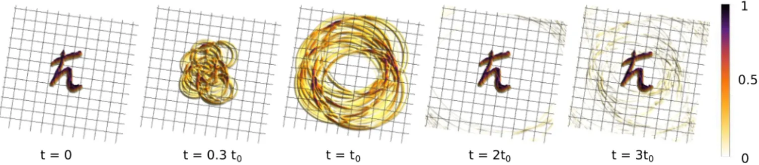
Here we show that it is indeed possible to devise high- fidelity (instantaneous) QTMs for the time evolution of wave functions. We propose a concept of QTMs based on (bosonic or fermionic) Dirac-like systems, such as graphene, exploiting the “population-reversal” principle at the heart of spin echoes. Indeed, this approach unifies two up to now distinct paradigms, the t inversion of a spatially extended wave and the generation of a (pseudo)spin echo. Figure 1 gives a taste of its effectiveness: An initially ¯h-shaped wave packet evolves in time progressively losing its profile, until the action of the instantaneous QTM, a short pulse att =t0, inverts the propagation and leads to a distinct echo att =2t0; the subsequent echo at t =3t0 is due to a further QTM pulse att=2.5t0(see movie in Supplemental Material [30]).
Experimentally there are various ways of injecting electronic wave packets—of simpler shape—into a system, notable ones including quantum dots as single-electron sources [31] or short voltage (“Leviton”) pulses [32].
FIG. 1. Echo in a Dirac quantum system. The absolute value of an ¯h-shaped wave packet is shown in real space (a.u.). The initial wave packet (att=0) becomes completely blurred while propagating untilt=t0. A fast quantum time-reversal pulse att=t0 leads to a nearly perfect echo att=2t0. The right panel (att=3t0) shows a second echo after a further subsequent pulse att=2.5t0. This simulation is done without disorder. The colorscale is the same in all snapshots, normalized to the highest value of the modulus of the initial wave packet.
II. QUANTUM TIME MIRROR BASICS
The two-dimensional (2D) Dirac system considered above could describe fermions in real [33] and artificial [34]
graphene, or, e.g., Dirac plasmons in metallic nanoparticle lattices [35] and polaritons in a honeycomb lattice [36]. In such systems the velocity is approximately constant—it does not depend on the k vector—and equal in magnitude, but opposite in direction, on the upper and lower Dirac cones.
Our t-inversion protocol aims at inducing a “population reversal,” say from the upper to the lower Dirac cone, which corresponds to an inversion of the velocity and thus effectively a propagation back in time. This is achieved by applying a short, spatially extended and (roughly) uniform perturbation opening a gap in the spectrum: Once initial upper cone states suddenly find themselves in the forbidden gap region, they start coherent oscillations between the upper and lower branches of the spectrum—akin to those responsible for Zitterbewegung. A proper tuning of such oscillations ensures that, by the time the perturbation is switched off and the gap closes, the states will end up in the lower Dirac cone [37].
A protocol of this kind must ensure that the initial wave function, an arbitrary coherent superposition of particlelike kmodes at different (positive) energies, keeps its shape while reforming as a coherent superposition of holelike k modes in the corresponding (negative) energy window, and that the probability for this “rigid” transition to the hole branch is as high as possible. As we will see, the linearity of the dispersion plays here the critical role. While the physical gap-opening mechanism depends on the Dirac-like system considered [38], its single crucial requirement is its nonadiabatic character as quantified below.
The effective Dirac Hamiltonian reads
H =ak·σ+M(t)σz=H0+H1, (1) where the mass term,
M(t)=
M0, t0< t < t0+t,
0, otherwise, (2)
acts as the time-dependent perturbation which temporarily opens a gap. The eigenenergies and eigenstates of H0 are Ek,±= ±akandψ±(k)= √12(±e1iθk), withθkthe polar angle in k space. During the pulse the eigenenergies of H are εk,±= ±√
M02+Ek,2±. In the time intervalt, an initialH0
eigenstate is subject to oscillations, whose cycle depends on the pulse strengthM0 and durationt. The amplitudeA to end up in the counterpropagatingH0eigenstate att=t0+t after the pulse can be tuned by adjusting both parameters. A straightforward calculation yields (see AppendixA)
A(k)= ψ±,k|e−hi¯H t |ψ∓,k
= − i
1+η2sin(μ
1+η2), (3) where we introduced the dimensionless parameters η= Ek,±/M0 and μ=M0t /¯h. The amplitude needs to be maximized for optimal echo strength, which then requires η1,μ≈π(n+1/2), n∈N0, corresponding to Ek,± M0≈πh/2t¯ for n=0. Notice that in a fermionic system the counterpropagating states need be empty. This is ensured, e.g., if the Fermi level (before injection of the wave packet) is such that F <−M0. The reversal amplitude (3) is weakly k dependent, a critical characteristic tied to the linearity of the dispersion [39], which suggests the QTM is highly effective in a widek/energy range. As we will see shortly, the numerical simulations confirm this. In general, given an initial wave packetψ(r,0)=(2π)−2
d2kψ(k,0)eik·r, a convenient measure of the echo strength is given by the correlation,
C(t)=
d2r|ψ(r,0)||ψ(r,t)|, (4) between the moduli of the amplitudes at times 0 andt.
To illustrate the QTM effect, a complicated wave packet resembling ¯h is numerically propagated in time (see Fig.1).
At times t0 and 2.5t0, a pulse with M0=8Ek and μ= M0t /¯h=π/2 is applied, withtt0. HereEk =akis the mean wave packet energy, i.e.,η =1/8. The snapshots in Fig.1demonstrate that even after full destruction the spatial distribution of the initial wave packet can be reconstructed.
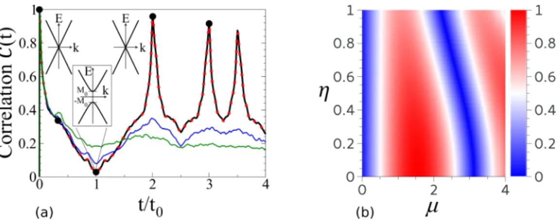
This is quantified and confirmed in Fig. 2(a), showing the corresponding correlator (4). At the echo time (t =2t0+ t≈2t0), major parts of the time propagated wave packet indeed return to the initial position. This QTM mechanism is not limited to a single pulse: Subsequent kicks att =2.5t0and t=3.25t0cause further peaks, albeit of decreasing size. The distinct echo peaks, based on the linear dispersion relation, arise since the kinetic phases accumulated by each k mode
FIG. 2. Quantitative analysis of the echo strength. (a) CorrelationC(t), Eq. (4), obtained from numerical propagation of the ¯hwave; see Fig.
1. Black circles mark the snapshot times. The solid black curve shows distinct echo peaks for the clean Dirac system, Eq. (1). The insets show sketches of the Dirac-type dispersion with a gap opening att=t0. Further curves correspond to different disorder types: gap disorder with τgap≈0.2t0 (red dotted), spatial disorder withτimp≈0.8t0(blue), andτimp≈0.2t0 (green).τimpandτgapare the respective elastic scattering times (see Sec.Bin the appendix). (b) Modulus|A(k)|of the transition amplitude, Eq. (3), plotted as a function of parametersηandμ.
during forward (0→t0) and backward (t0+t →2t0+t) propagation add up to zero (see AppendixA).
The numerical simulations are based on the wave packet propagation algorithm time-dependent quantum transport (TQT) [40]. The state is discretized on a square grid and the time evolution is calculated for sufficiently small time steps such that the Hamilton operator can be assumed time independent for each step. We calculate the action ofHonψ in a mixed position and momentum-space representation by the application of Fourier transforms. With this a Krylov space is spanned, which can be used to calculate the time evolution using the Lanczos method [41].
For an arbitrary wave packet, the echo strengthC(2t0+t) is analytically given solely in terms of the amplitude A(k), Eq. (3), and the wave packet att =0 as
C(2t0+t)=
d2r|ψ(r,0)|
d2k
(2π)2A(k)ψ(k,0)eik·r . (5) Figure 2(b) shows the η and μ dependence of |A(k)|, obtained from the time-reversal amplitude (3). One finds extended stripes of high fidelity. To check this analytical result we simulate the propagation of a normalized 2D Gaussian wave packet with positive energy and small k-space width kk0compared to the absolute valuek0of its mean wave vector, such that A(k)≈A(k0) for all k modes involved.
Under these assumptions, Eq. (5) reduces to C(2t0+t)≈
|A(k0)| (see AppendixA), which can be compared with the correlationC(2t0+t), Eq. (4), obtained from full numerical time evolution. As the mean difference between analytics and numerics is 0.03, only the analytical plot is shown.
Clearly, strong echoes can be obtained in the full energy range 0η1.
III. DISORDER
We now investigate the QTM robustness against disorder.
While this is typically present in a real system, it should be emphasized that state-of-the-art hBN-encapsulated graphene samples are effectively ballistic over scales of several microns
[42], corresponding to (transport) scattering times of several picoseconds. For the sake of clarity, we keep the discussion at a qualitative level and refer the reader to AppendixBfor quantitative details.
We consider two types of disorder: a static spatial disorder potential and a spatially random pulse strength (referred to as “gap disorder”). Spatial disorder enters into the Hamilto- nian (1) as a time- and (pseudo)spin-independent potential Vimp(r)σ0, whereσ0 is the unit matrix in (pseudo)spin space.
Gap disorder is instead given byVgap(r)σzfort ∈[t0,t0+t], i.e., only during the pulse. Both random potentials are Gaussian distributed with widthuimporugap.
As shown in Fig.2(a), the echo is clearly more sensitive to a static random impurity potential than to gap disorder. This is expected, and can be understood within the framework of Loschmidt echo theory [12,43,44]: If a t-inversion protocol is not perfect, the echo signal decays as a function of the propagation time t0. Spatial disorder reduces the fidelity, since the QTM mechanism, even for an optimally calibrated pulse, achieves “population reversal” without directly affecting the impurity scattering dynamics. In other words, the QTM protocol does not lead toVimp(r)→ −Vimp(r). In this sense elastic disorder has a qualitatively similar effect to inelastic scattering, whose effects are also not undone by the QTM.
Gap disorder plays in principle a similar QTM-breaking role. However, and contrary to spatial disorder, it is active only during the very short pulse duration timett0 and thus causes only negligible echo losses, reflected in the perfect agreement of the black line and dotted red line in Fig.2(a).
Our analysis also highlights a fundamental difference between standard spin echoes and the present wave function echo: While a spin echo decays because of dynamical (inelas- tic) perturbations leading toT2, the role ofT2is here played by the elastic scattering timeτ. This suggests an application of the QTM as a probe of the quality of a sample—much as the spin echo is used as a probe of decoherence in two-level systems.
We now explain at a qualitative level how and why static (elastic) disorder affects our echo, whereas spin echoes are insensitive to it. First, consider the scattering off a single impurity, assuming an incoming plane wave with a given
propagation direction ˆv. Scattering leads to a position- dependent change of the wave front propagation direction.
Considering true time reversal after the scattering process, every scattered part of the wave propagates back to the impurity and is scattered again. However, due to destructive interference only the (inverted) initial propagation direction−vˆsurvives.
In the presence of many scatterers, a Feynman path approach provides convenient insights. While a phase ϕs is accumulated along one particular pathsdue to scattering off impurities, the same phase with inverted sign−ϕs is picked up on the way back, after (perfect) time inversion due to the time-reversal operator T ∝Cσy, where C indicates complex conjugation. Every backward pathsother than the original one leads to a different phase−ϕs = −ϕs. This causes destructive interference and ensures that only the contribution from the original pathssurvives.
This phase inversion is also achieved in spin echoes.
Depending on the environment, the spins precess slower or faster. By applying aπpulse at timet0which flips the spin, the faster spins are “suddenly behind” the slower ones. Neglecting inelastic effects, all spins are in phase again at 2t0 leading to the Hahn echo [3].
As opposed to the discussion about perfect time reversal, our pulse does not define an exactt-inversion protocol even in the absence of inelastic scattering, since it only inverts (“flips”) the kinetic phase due to H0, which is e−iE±t0/¯h. Without disorder this is the only phase present, and thus it disappears for a closed loop (forward, then backward) propagation (see AppendixA). With disorder the phase due to the random potentialVimp(r) is not inverted and therefore not canceled after the pulse on the way back. This leads to a “dephasing,” such that contributions from various pathss survive at each impurity as opposed to the perfect time reversal discussed above, where only the time-reversed counterpart of the incoming path survives.
IV. CONCLUSIONS
The analytical and numerical considerations presented in this work confirm the principles behind our QTM for pseudorelativistic graphenelike systems. This means that a sufficiently fast and spatially extended perturbation which opens a gap in a Dirac system can act similar to a microwave π pulse in spin-echo experiments, effectively t inverting the orbital wave function dynamics and thus generating a wave function echo.
It is important to remark that the QTM does not require time-reversal symmetry to be preserved. Indeed, we checked both analytically and numerically that high-fidelity echoes can also be obtained, e.g., in graphene in the presence of a constant perpendicular magnetic field B= ∇ ×A, described by the HamiltonianH=a[k−(e/¯h)A]·σ+M(t)σz.Wave packets in this case consist of superpositions of Landau levels with discrete energiesEn,±∝ ±√
n[45,46], while during the pulse the dispersion becomes εn,±=√
M02+En,2±. The analogy with the discussion of Eq. (1) is evident, and in fact for each electronlike (upper Dirac branch) Landau level, the transition amplitude to its holelike (lower Dirac branch) equivalent is again given by Eq. (3), where nowη=En,±/M0. Since the propagation directions of electron- and holelike Landau levels
are reversed, the QTM principle still applies, and strong echoes are obtained for 0η1.
The fact that time-reversal invariance need not be preserved may allow a further twist to the QTM proposal. The idea is to exploit the orbital effects of a pulsed out-of-plane magnetic field, rather than a mass gap pulse: When the magnetic field is switched on the Dirackdispersion is abruptly changed to a gapped Landau level spectrum, suggesting the feasibility of a Landau level-based QTM [47].
Various experimental realizations of the QTM proposed here can be imagined. Our QTM represents a general proof of concept, based on a single-particle picture and including the assumption that the inelastic relaxation time of the injected wave packet is larger thant0. This condition imposes certain restrictions in real graphene [48–50], though femtosecond laser pulses, routinely employed in nanospectroscopy [51], could be employed to open gaps therein, and indeed recent experimental advances suggest such restrictions not to be critical [52]. On the other hand, certain forms of artificial graphene [34,36] could be amenable to a straightforward experimental implementation of the QTM. We also note that similar physics can be expected in the surface states of three-dimensional topological insulators [53], though this will be discussed elsewhere.
We furthermore demonstrated that thet-inversion protocol does not require time-reversal symmetry and is practically insensitive to pulse (gap) disorder. Vice versa, QTM-based echo spectroscopy could be used as a sensitive local probe of elastic and inelastic scattering times in Dirac-type systems.
In summary, we have proposed an instantaneous QTM for an extended quantum state, based on the pseudorelativistic dispersion of (bosonic or fermionic) Dirac-like systems. An experimental realization of such an echo mechanism is within reach in state-of-the-art real or artificial graphene.
ACKNOWLEDGMENTS
We thank R. Huber for useful discussions. A.G. acknowl- edges the support of EPSRC Grant No. EP/K024116/1. C.G., V.K., K.R., and P.R. acknowledge support from Deutsche Forschungsgemeinschaft within SFB 689 and GRK 1570.
APPENDIX A: DERIVATION OF TRANSITION PROBABILITY TO COUNTERPROPAGATING
EIGENSTATE
We first derive Eq. (3) describing the transition amplitude owing to a time-dependent pulse in a Dirac-type system. The effective Hamiltonian for graphenelike (single-cone) systems is given by Eqs. (1) and (2). The eigenenergies and eigenstates ofH0are
E±= ±ak, (A1)
ψ±(k)= 1
√2 1
±e+iθk
, (A2)
whereθkis the polar angle inkspace. During the time interval t, an initialH0eigenstate is subject to Rabi-like oscillations, whose cycle depends on the pulse’s strengthM0 and length
t. The new eigenenergies and states become
ε±= ± a2k2+M02, (A3) χ±(k)= 1
a2k2+(M0+ε±)2
M0+ε± ak e+iθk
. (A4) Thus, a band gap opens atk=0 with width=2M0.
The time evolution is explicitly performed for one mode, so as to derive the transition probability. Consider, an initial eigenstate with negative energy|φk(t=0) = |ψ−k. The index kis from now on omitted for sake of brevity. The time evolution up tot=t0 is trivial and results in a global phase:|φ(t) = e−hi¯E−t0|ψ−. During the pulse, the time evolution is governed byH, therefore we decompose|ψ−into eigenstates|χ±:
|ψ− =
s=±
αs|χs, (A5) with
αs = χs |ψ−, (A6) and the time evolution from t=t0 to t =t0+t =t1 becomes
|φ(t1) =e−hi¯E−t0e−¯hiH t|ψ−
=e−hi¯E−t0
s=±
αse−hi¯εst|χs. (A7) We are interested only in the component propagating back to its initial position, thus we project |φ(t1) onto|ψ+, which has opposite velocity as compared to the initial state,
ψ+|φ(t1) =e−h¯iE−t0
s=±
αse−hi¯εstψ+|χs
=e−h¯iE−t0
s=±
αse−hi¯εstβs∗, (A8) with
βs= χs |ψ+. (A9) The component ψ−|φ(t1) keeps propagating in its initial direction and is lost for the echo.
The echo takes place at t2=2t0+t2t0 (t t0), because the absolute value of the velocity is the same for|ψ+ and|ψ−. The last propagation step tot2 is again trivial and yields an additional phasee−hi¯E+t0for the component traveling back, which cancels with the phase fromt =0 tot =t0(E+=
−E−). The echo amplitude thus reads ψ+|φ(t2) =
s=±
αsβs∗e−hi¯εst. (A10) Inserting the explicit expressions for αs, βs, and εs, a straightforward but tedious calculation yields
ψ+|φ(t2) = − i 1+aM2k22
0
sin M0t
¯ h
1+a2k2 M02
= − i
1+η2sin(μ
1+η2), (A11)
where the dimensionless parameters η=ak/M0 and μ= M0t /¯h were introduced. Equation (A11) corresponds to Eq. (3). The trivial time evolutions before and after the pulse cancel each other in the absence of disorder, so that the echo strength is solely due to the (modulus of the) transition amplitude to the counterpropagating eigenstate.
Starting in|ψ+ instead of|ψ−, or in a superposition of the two, leads to the same conclusions.
For an arbitrary initial wave packet φ(r,0)= (2π)−2
d2kφ(k,0)eik·r, the simulation-derived echo strength C(2t0) can be analytically estimated. In Eqs. (A5)–(A11), we solve the Schr¨odinger equation exactly for the population-reversed part of the wave packet, i.e., the only part contributing to the echo is
φ(k,2t0+t)=A(k)φ(k,0), (A12) and therefore in real space,
φ(r,2t0+t)= d2k
(2π)2 φ(k,2t0)eik·r
= d2k
(2π)2 A(k)φ(k,0)eik·r. (A13) As noted, the kinetic phases accumulated before and after the pulse cancel at t =2t0+t2t0, preventing interference effects in real space. Moreover, the linear band structure with constant phase velocity keeps the shape of the wave packet.
Thus, our analytical estimate yields C(2t0)=
d2r|φ(r,0)||φ(r,2t0)|
=
d2r|φ(r,0)|
d2k
(2π)2A(k)φ(k,0)eik·r
=:CA, (A14)
which is the same as Eq. (5).
In case of nearly constantA(k)≈A(k0), e.g., for narrow peaked wave packets inkspace around an average valuek0, the echo strength can be estimated by
C(2t0)≈
d2r|φ(r,0)|
d2k
(2π)2 A(k0)φ(k,0)eik·r
=A(k0)
d2r|φ(r,0)| |φ(r,0)| =A(k0), (A15) having taken a normalized initial wave packet.
APPENDIX B: DISORDER EFFECTS TO THE ECHO 1. Spatial disorder
For the numerical investigation of disorder effects, we use a random, pseudospin-independent potentialVimp(r)σ0. The latter assigns to every grid pointia normally distributed value βi, which is then multiplied with the disorder strengthuimp. The discontinuous potential is then smoothed by a Gaussian distribution with widthl0. This leads to
Vimp(r)= uimp N
i
βie−
(r−ri)2 l2
0 , (B1)
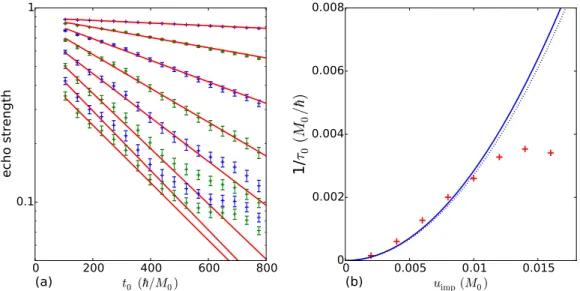
FIG. 3. Effects of disorder on graphene echo. (a) The echo strength measured by the echo fidelity ˜M(techo) is shown as a function of pulse timet0for various disorder strengthsuimpbetween 0.002M0and 0.016M0, averaged over 50 realizations (see text). The error bars denote the standard error of the mean. An exponential fit is used to extract the decay rate. For higheruimpan expected saturation sets in, such that only a brief regime of exponential decay is visible. (b) Plot of the fitted decay rates 1/τ0as a function ofuimp, Eq. (B5), which is quadratic for weak scattering. The black dotted line is the analytically expected curve, which matches well the fitted quadratic function (blue), until the expected strong scattering saturation sets in.
where the sum runs over all grid points. The normalizationN is due to numerical reasons and is given by
N =
⎡
⎣1 A
A
d2r
i
βie−
(r−ri)2 l2
0
2⎤
⎦
1 2
, (B2) Abeing the (finite) grid area for the numerical simulation. The correlator,
Vimp(r)Vimp(r) =u2impe−
(r−r)2 2l2
0 , (B3)
where · stands for disorder average, is needed in order to compute the scattering time. The latter is given by (see, e.g., [54])
¯ h τk =
dkdr
2πh¯ δ(k−k)Vimp(0)Vimp(r)eir·k, (B4) and can be calculated analytically as
1 τk = 2π
a¯hu2impl02k e−l20k2I0 l02k2
. (B5)
I0(x) is the modified Bessel function of zeroth kind.
In the main part, we explained on a qualitative level the effect of disorder. Here, we discuss it quantitatively and for that reason we turn to the theory of Loschmidt echoes (see, e.g., [43,44,55,56]), where the role of disorder has been thoroughly studied and characterized. In this context the echo is measured by the “fidelity,”
M(t)= |φ|eiHat/¯he−iHbt/¯h|φ|2, (B6) which is the overlap squared between the initial and final, i.e., time-evolved, state. The time propagation is governed byHb until the timet, and by−Hathereafter, i.e., the time evolution is (“by hand”) explicitly inverted. (Note the difference to our
protocol where the flow in time is not changed.) Moreover, we use instead the correlationC(t), Eq. (4), to quantify the echo in a physically transparent way—as the overlap between initial and time-evolved local density. In order to establish a connection with the Loschmidt echo theory, it is, however, more convenient to introduce the following “echo fidelity” ˜M, M(t˜ )= |σzφ|e−iH t/¯h|φ|. (B7) Notice the difference withC(t), where|φ|appears, and theσz
Pauli matrix: ˜M(t) is the overlap of the time propagated state with the initial onewith flipped spinor, since the returning part of the wave packet is in the flipped eigenstate ofH0. In the golden rule decay regime [44], the (mean) echo strength ˜M decays exponentially in time,
M(t˜ )∼e−2τt . (B8) As mentioned, the pulse time reverses the dynamics due toH0 only, without affecting the dynamics arising from the impurity potential. This can be seen by splitting the time evolution operator in three parts: before the pulse, during the pulse, and after the pulse. Furthermore, we consider only the part of the wave function which is reflected, which means that the time evolution during the pulse is given by the transition amplitudeA(k) times the operatorσz, which maps any state to its energy-inversed counterpart.
M(2t˜ 0)= |φ|σze−hi¯(H0+Vimp)t0σzA(k)e−hi¯(H0+Vimp)t0|φ|2
= |φ|e−hi¯σz(H0+Vimp)σzt0A(k)e−hi¯(H0+Vimp)t0|φ|2. (B9) Sinceσzσiσz= −σi fori∈ {x,y}andH0 is a linear combi- nation ofσx andσy, the sign in front ofH0changes after the pulse, whereas the term related to the pseudospin-independent
potentialVr is not affected at all by the pulse.
M(2t˜ 0)= |φ|e−hi¯(−H0+Vimp)t0A(k)e−hi¯(H0+Vimp)t0|φ|2. (B10) As there is a different sign in the propagation due toH0before and after the pulse, there iseffectivelya propagation backwards in time. On the other hand, ourσzpulse cannot invert the time evolution due to the disorder potential, which causes disorder to ultimately destroy the echo.
Since the scattering occurs during the whole propagation time 2t0, we expect the echo fidelity (B8) to decay as
M(2t˜ 0)∼e−2t2τ0 =e−tτ0. (B11) This decay is confirmed in Fig.3(a), where the echo fidelity (=echo strength), Eq. (B7), is shown as a function of the pulse timet0. The initial wave packet is a 2D Gaussian with small k-space widthσkk0as compared to the mean wave vector k0, such that thekdependence of the scattering time can be neglected (τk≈τk0 =:τ0). The echo strength is calculated for 50 different realizations of the random disorder potential and averaged subsequently. For large disorder strengths uimp, a saturation regime is reached, in accordance with Loschmidt echo theory [44]. The decay rate is extracted by fitting an
exponentially decaying function to the data, and compared in Fig.3(b) to the analytically expected decay rate 1/τ0 from Eq. (B5), yielding a good agreement.
The time decay of C(t) is qualitatively similar though slower, because the phase differences between the initial and the propagated wave packet are neglected in the modulus, preventing eventual destructive interference.
2. Gap disorder
The gap disorder potentialVgap(r)σzmodels fluctuations in the pulse strength and is therefore only active in the short time windowt. Figure2(a)shows that gap disorder has practically no effect on the echo as compared to spatial disorder. This is expected, as spatial disorder is active during a time 2t0t.
Assuming similar scattering times foruimp=ugap, practically no gap disorder-induced scattering takes place during the pulse, sinceτ0t. Moreover, spatial and gap disorder acts slightly differently. The impurities lead to a randomization of the propagation direction, such that a smaller amount of the wave packet goes back to the initial position. Gap disorder instead modulates in space the transition probability to the counterpropagating eigenstate, but the propagation direction is not randomized.
[1] J. Loschmidt, ¨Uber den Zustand des W¨armegleichgewichts eines Systems von K¨orpern mit R¨ucksicht auf die Schwerkraft, Sitzungberichte der Akademie der Wissenschaften II, 128 (1876).
[2] L. Boltzmann, ¨Uber die Beziehung eines allgemeinen mech- anischen Satzes zum zweiten Hauptsatze der W¨armetheorie, Sitzungberichte der Akademie der WissenschaftenII, 67 (1877).
[3] E. L. Hahn, Spin echoes,Phys. Rev.80,580(1950).
[4] J. A. Weil and J. R. Bolton,Electron Paramagnetic Resonance (John Wiley & Sons, New York, 2007).
[5] M. Fink, Time reversal of ultrasonic fields. I. Basic princi- ples, IEEE Transactions on Ultrasonics, Ferroelectrics, and Frequency Control39,555(1992).
[6] C. Draeger and M. Fink, One-Channel Time Reversal of Elastic Waves in a Chaotic 2D-Silicon Cavity,Phys. Rev. Lett.79,407 (1997).
[7] M. Fink, Time reversed acoustics,Physics Today50,34(1997).
[8] G. Lerosey, J. de Rosny, A. Tourin, A. Derode, G. Montaldo, and M. Fink, Time Reversal of Electromagnetic Waves,Phys.
Rev. Lett.92,193904(2004).
[9] A. Przadka, S. Feat, P. Petitjeans, V. Pagneux, A. Maurel, and M. Fink, Time Reversal of Water Waves,Phys. Rev. Lett.109, 064501(2012).
[10] A. Chabchoub and M. Fink, Time-Reversal Generation of Rogue Waves,Phys. Rev. Lett.112,124101(2014).
[11] H. M. Pastawski, E. P. Danieli, H. L. Calvo, and L. E. F. Foa Torres, Towards a time reversal mirror for quantum systems, EPL77,40001(2007).
[12] H. L. Calvo, R. A. Jalabert, and H. M. Pastawski, Semiclassical Theory of Time-Reversal Focusing,Phys. Rev. Lett.101,240403 (2008).
[13] H. L. Calvo and H. M. Pastawski, Exact time-reversal focusing of acoustic and quantum excitations in open cavities: The perfect inverse filter,EPL89,60002(2010).
[14] A. P. Mosk, A. Lagendijk, G. Lerosey, and M. Fink, Controlling waves in space and time for imaging and focusing in complex media,Nat. Phot.6,283(2012).
[15] A. Yariv, Four wave nonlinear optical mixing as real time holography,Opt. Commun.25,23(1978).
[16] D. A. B. Miller, Time reversal of optical pulses by four-wave mixing,Opt. Lett.5,300(1980).
[17] M. Moshinsky, Diffraction in time,Phys. Rev.88,625(1952).
[18] A. S. Gerasimov and M. V. Kazarnovskii, Possibility of observing nonstationary quantum-mechanical effects by means of ultracold neutrons, Sov. Phys. JETP44, 892 (1976).
[19] ˇC. Brukner and A. Zeilinger, Diffraction of matter waves in space and in time,Phys. Rev. A56,3804(1997).
[20] J. T. Mendonc¸a and P. K. Shukla, Time refraction and time reflection: Two basic concepts, Phys. Scripta 65, 160 (2002).
[21] A. del Campo, G. Garcia-Calder´on, and J. G. Muga, Quantum transients,Phys. Rep.476,1(2009).
[22] A. Goussev, Huygens-Fresnel-Kirchhoff construction for quan- tum propagators with application to diffraction in space and time,Phys. Rev. A85,013626(2012).
[23] P. Haslinger, N. Dorre, P. Geyer, J. Rodewald, S. Nimmrichter, and M. Arndt, A universal matter-wave interferometer with optical ionization gratings in the time domain, Nat. Phys.9, 144(2013).
[24] J. Martin, B. Georgeot, and D. L. Shepelyansky, Cooling by Time Reversal of Atomic Matter Waves,Phys. Rev. Lett.100, 044106(2008).
[25] J. Martin, B. Georgeot, and D. L. Shepelyansky, Time Reversal of Bose-Einstein Condensates, Phys. Rev. Lett.101, 074102 (2008).
[26] A. Ullah and M. D. Hoogerland, Experimental observation of Loschmidt time reversal of a quantum chaotic system,Phys.
Rev. E83,046218(2011).
[27] Y. Sivan and J. B. Pendry, Time Reversal in Dynamically Tuned Zero-gap Periodic Systems,Phys. Rev. Lett.106,193902 (2011).
[28] Y. Sivan and J. B. Pendry, Theory of wave-front reversal of short pulses in dynamically tuned zero-gap periodic systems, Phys. Rev. A84,033822(2011).
[29] V. Bacot, M. Labousse, A. Eddi, M. Fink, and E. Fort, Time reversal and holography with spacetime transformations,Nat.
Phys.12,972(2016).
[30] See Supplemental Material athttp://link.aps.org/supplemental/
10.1103/PhysRevB.95.165421for a video of QTM pulse action.
[31] E. Bocquillon, V. Freulon, F. D. Parmentier, J.-M. Berroir, B.
Plac¸ais, C. Wahl, J. Rech, T. Jonckheere, T. Martin, C. Grenier, D. Ferraro, P. Degiovanni, and G. F`eve, Electron quantum optics in ballistic chiral conductors,Ann. Phys. (Berlin)526,1 (2014).
[32] T. Jullien, P. Roulleau, B. Roche, A. Cavanna, Y. Jin, and D. C.
Glattli, Quantum tomography of an electron,Nature (London) 514,603(2014).
[33] A. H. Castro Neto, F. Guinea, N. M. R. Peres, K. S. Novoselov, and A. K. Geim, The electronic properties of graphene,Rev.
Mod. Phys.81,109(2009).
[34] L. Tarruell, D. Greif, T. Uehlinger, G. Jotzu, and T. Esslinger, Creating, moving and merging Dirac points with a Fermi gas in a tunable honeycomb lattice,Nature (London)483,302(2012).
[35] G. Weick, C. Woollacott, W. L. Barnes, O. Hess, and E. Mar- iani, Dirac-Like Plasmons in Honeycomb Lattices of Metallic Nanoparticles,Phys. Rev. Lett.110,106801(2013).
[36] T. Jacqmin, I. Carusotto, I. Sagnes, M. Abbarchi, D. D.
Solnyshkov, G. Malpuech, E. Galopin, A. Lemaˆıtre, J. Bloch, and A. Amo, Direct Observation of Dirac Cones and a Flatband in a Honeycomb Lattice for Polaritons,Phys. Rev. Lett.112, 116402(2014).
[37] In fermionic systems such lower cone states must be available, i.e., they should not be already occupied; see discussion following Eq. (3).
[38] For example, gaps in real graphene can be dynamically opened and closed via THz radiation [57–59]. A further experimental example of ultrafast manipulation of the graphene spectrum appears in Ref. [52].
[39] The QTM principle works also in nonlinear dispersions, though less effectively. A discussion of this physics will appear elsewhere.
[40] V. Kr¨uckl, Wave packets in mesoscopic systems: From time- dependent dynamics to transport phenomena in graphene and topological insulators, Ph.D thesis, Universit¨at Regensburg, Regensburg, Germany (2013); the basic version of the algorithm is available at TQT Home [http://www.krueckl.de/#en/tqt.php].
[41] C. Lanczos, An iteration method for the solution of the eigenvalue problem of linear differential and integral operators, J. Res. Natl. Bur. Stand.45,255(1950).
[42] L. Wang, I. Meric, P. Y. Huang, Q. Gao, Y. Gao, H. Tran, T.
Taniguchi, K. Watanabe, L. M. Campos, D. A. Muller, J. Guo, P. Kim, J. Hone, K. L. Shepard, and C. R. Dea, One-dimensional electrical contact to a two-dimensional material,Science342, 614(2013).
[43] R. A. Jalabert and H. M. Pastawski, Environment-Independent Decoherence Rate in Classically Chaotic Systems,Phys. Rev.
Lett.86,2490(2001).
[44] A. Goussev, R. A. Jalabert, H. M. Pastawski, and D. A.
Wisniacki, Loschmidt echo,Scholarpedia7,11687(2012).
[45] J. W. Clure, Diamagnetism of graphite,Phys. Rev.104, 666 (1956).
[46] M. O. Goerbig, Electronic properties of graphene in a strong magnetic field,Rev. Mod. Phys.83,1193(2011).
[47] P. Recket al., (unpublished).
[48] A. Urich, K. Unterrainer, and T. Mueller, Intrinsic response time of graphene photodetectors,Nano Lett.11,2804(2011).
[49] J. C. W. Song and L. S. Levitov, Energy flows in graphene:
hot carrier dynamics and cooling,J. Phys.: Condens. Matter27, 164201(2015).
[50] K. J. Tielrooij, L. Piatkowski, M. Massicotte, A. Woessner, Q.
Ma, Y. Lee, K. S. Myhro, C. N. Lau, P. Jarillo-Herrero, N. F.
van Hulst, and F. H. L. Koppens, Generation of photovoltage in graphene on a femtosecond timescale through efficient carrier heating,Nature Nanotech.10,437(2015).
[51] M. Eisele, T. L. Cocker, M. A. Huber, M. Plankl, L. Viti, D.
Ercolani, L. Sorba, M. S. Vitiello, and R. Huber, Ultrafast multi- terahertz nano-spectroscopy with sub-cycle temporal resolution, Nat. Photon.8,841(2014).
[52] T. Higuchi, C. Heide, K. Ullmann, H. B. Weber, and P. Hommel- hoff, Light-field driven currents in graphene,arXiv:1607.4198.
[53] M. Z. Hasan and C. L. Kane, Colloquium: Topological insula- tors,Rev. Mod. Phys.82,3045(2010).
[54] E. Akkermans and G. Montambaux, Mesoscopic Physics of Electrons and Photons (Cambridge University Press, Cam- bridge, 2007).
[55] Ph. Jacquod, P. G. Silvestrov, and C. W. J. Beenakker, Golden rule decay versus Lyapunov decay of the quantum Loschmidt echo,Phys. Rev. E64,055203(2001).
[56] N. R. Cerruti and S. Tomsovic, Sensitivity of Wave Field Evolution and Manifold Stability in Chaotic Systems, Phys.
Rev. Lett.88,054103(2002).
[57] M. V. Fistul and K. B. Efetov, Electromagnetic-field-induced Suppression of Transport Through n-p Junctions Graphene, Phys. Rev. Lett.98,256803(2007).
[58] A. Scholz, A. L`opez, and J. Schliemann, Interplay between spin- orbit interactions and a time-dependent electromagnetic field in monolayer graphene,Phys. Rev. B88,045118(2013).
[59] G. Usaj, P. M. Perez-Piskunow, L. E. F. Foa Torres, and C. A.
Balseiro, Irradiated graphene as a tunable floquet topological insulator,Phys. Rev. B90,115423(2014).