(Dated: January 8, 2018)
Both metaphysical and practical considerations related to time inversion have intrigued scientists for generations. Physicists have strived to devise and implement time-inversion protocols, in par- ticular different forms of “time mirrors” for classical waves. Here we propose an instantaneous time mirror forquantum systems,i.e. a controlled time discontinuity generating wave function echoes with high fidelities. This concept exploits coherent particle-hole oscillations in a Dirac spectrum in order to achieve population reversal, and can be implemented in systems such as (real or artificial) graphene.
I. INTRODUCTION
The physicists’ fascination with time inversion goes back a long time, as testified by the famous 19th-century argument between Loschmidt and Boltzmann concern- ing the arrow of time [1, 2]. Deep theoretical and meta- physical considerations are not the sole reasons behind it, though. The pioneering work of Hahn in 1950 [3], in which the dynamics of an ensemble of nuclear spins was successfully time inverted, gave birth to the concept of spin echo, now central to numerous imaging techniques [4]. A spin echo, at least in its most basic form, can be understood in terms of “population reversal” in two-level systems: an ensemble of initially uniformly aligned spins precesses around an applied magnetic field, progressively losing relative phase coherence; a microwave π-pulse is then used to simultaneously flip the spins, making them effectively evolve “back in time” regaining (“echoing”) the initially aligned, phase coherent configuration.
Another successful approach to time inversion has been developed for classical waves based on time-reversal mir- rors implemented with acoustic [5, 6], elastic [7], electro- magnetic [8] and recently water waves [9, 10]. It relies on the fact that any wave field can be completely de- termined in a volume by knowing only the field at any enclosing surface (a spatial boundary). It requires the use of receiver-emitter antennas positioned on the surface that record an incident wavefront and later rebroadcast a time-inverted copy of the signal. If an initially local- ized pulse, e.g. a wave emitted from any source, is left to evolve for a certain time and then in this manner t- inverted on a boundary, it can trace its way back to the initial source and there refocus or “echo” [11–13]. This process is difficult to implement in optics because of the lack of controllable antennas [14], and a solution to cre- ate time-reversed waves is to work with monochromatic light and use three- or four-wave mixing [15, 16].
A potent alternative to wave field control via spatial boundaries is the manipulation of time boundaries [17–
23]. Specific time reversal protocols for one-dimensional (1D) propagation were proposed [24, 25] and experimen- tally realized [26] in the kicked rotator model of atomic
matter waves (for a narrow range of momenta), and pro- posed for electromagnetic waves [27, 28], the latter based on time- and space-modulated perturbations of a pho- tonic crystal with linear dispersion. The latest develop- ment in this context is the concept of an instantaneous time mirror, which has been verified experimentally [29]
in the field of gravity-capillary waves: A sudden modifi- cation of water wave celerity obtained from a vertical ac- celeration of a bath of water creates a time-reversed wave.
This time disruption realizes an instantaneous time mir- ror in the entire space. Such a mirror can be viewed as the analogue in time to a standard mirror that acts on space.
In spite of these successes for classical waves, a long standing challenge remains: are Quantum Time Mirrors (QTMs) feasible for spatially extended quantum waves?
In other words, can one time-invert the motion of a quan- tum wave propagating in space? Notice that unlike spin echoes, which deal with (an ensemble of) discrete two- level systems, one is here dealing with a continuous de- gree of freedom describing a wave function extending and evolving coherently in space. A direct adaption of the aforementioned classical wave strategies appears difficult:
On the one hand, recording and properly re-emitting waves would require to measure and thereby massively change the quantum state; on the other hand, the in- triguing concept of a time mirror for water waves cannot be transferred to wave functions due to the inherently dif- ferent structure of the underlying differential equations describing classical and quantum wave propagation.
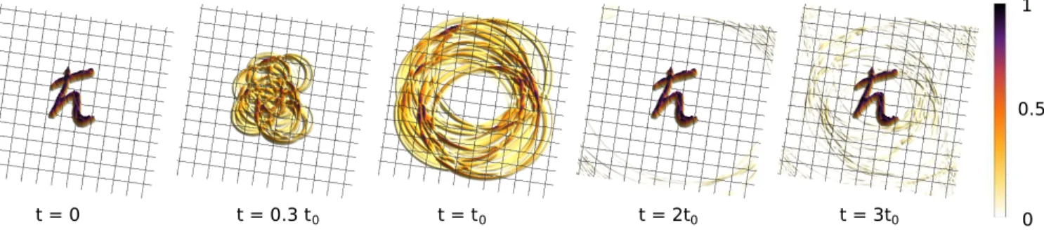
Here we show that it is indeed possible to devise high- fidelity (instantaneous) QTMs for the time evolution of wave functions. We propose a concept of QTMs based on (bosonic or fermionic) Dirac-like systems, such as graphene, exploiting the “population reversal” principle at the heart of spin echoes. Indeed, this approach uni- fies two up to now distinct paradigms, the t-inversion of a spatially extended wave and the generation of a (pseudo)spin echo. Figure 1 gives a taste of its effective- ness: an initially ~-shaped wave packet evolves in time progressively losing its profile, until the action of the in- stantaneous QTM, a short pulse at t = t0, inverts the
arXiv:1603.07503v2 [cond-mat.mes-hall] 3 Jan 2018
FIG. 1. Echo in a Dirac quantum system. The absolute value of a ~-shaped wave packet is shown in real space (a.u.). The intial wave packet (att= 0) becomes completely blurred while propagating untilt=t0. A fast quantum time reversal pulse att=t0 leads to a nearly perfect echo att= 2t0. The right panel (att= 3t0) shows a second echo after a further subsequent pulse at t= 2.5t0. This simulation is done without disorder. The colorscale is the same in all snapshots, normalized to the highest value of the modulus of the initial wave packet.
propagation and leads to a distinct echo att = 2t0; the subsequent echo att= 3t0is due to a further QTM pulse at t = 2.5t0 (see movie in [30]). Experimentally there are various ways of injecting electronic wave packets – of simpler shape – into a system, notable ones includ- ing quantum dots as single-electron sources [31] or short voltage (“Leviton”) pulses [32].
II. QUANTUM TIME MIRROR - BASICS The two-dimensional (2D) Dirac system considered above could describe fermions in real [33] and artifi- cial [34] graphene, or e. g. Dirac plasmons in metallic nanoparticle lattices [35] and polaritons in a honeycomb lattice [36]. In such systems the velocity is approximately constant – it does not depend on thek-vector – and equal in magnitude, but opposite in direction, on the upper and lower Dirac cones. Our t-inversion protocol aims at in- ducing a “population reversal”, say from the upper to the lower Dirac cone, which corresponds to an inversion of the velocity and thus effectively a propagation back in time.
This is achieved by applying a short, spatially extended and (roughly) uniform perturbation opening a gap in the spectrum: Once initial upper cone states suddenly find themselves in the forbidden gap region, they start coher- ent oscillations between the upper and lower branches of the spectrum – akin to those responsible for Zitter- bewegung. A proper tuning of such oscillations ensures that, by the time the perturbation is switched off and the gap closes, the states will end up in the lower Dirac cone. [37] A protocol of this kind must ensure that the initial wave function, a arbitrary coherent superposition of particle-like k-modes at different (positive) energies, keeps its shape while reforming as a coherent superposi- tion of hole-likek-modes in the corresponding (negative) energy window, and that the probability for this “rigid”
transition to the hole branch is as high as possible. As we will see, the linearity of the dispersion plays here the
critical role. While the physical gap-opening mechanism depends on the Dirac-like system considered [38], its sin- gle crucial requirement is its non-adiabatic character as quantified below.
The effective Dirac Hamiltonian reads
H=ak·σ+M(t)σz=H0+H1, (1) where the mass term
M(t) =
M0, t0< t < t0+ ∆t,
0, otherwise, (2)
acts as the time-dependent perturbation which temporar- ily opens a gap. The eigenenergies and eigenstates ofH0 areEk,±=±akandψ±(k) = √1
2
1
±eiθk
, withθkthe polar angle ink-space. During the pulse the eigenenergies ofH areεk,± =±q
M02+Ek,±2 . In the time interval ∆t, an initialH0 eigenstate is subject to oscillations, whose cycle depends on the pulse strengthM0and duration ∆t.
The amplitude A to end up in the counter-propagating H0eigenstate att=t0+ ∆tafter the pulse can be tuned by adjusting both parameters. A straightforward calcu- lation yields (see Appendix A)
A(k) =hψ±,k|e−~iH∆t|ψ∓,ki
=− i
p1 +η2sin µp
1 +η2
, (3)
where we introduced the dimensionless parameters η = Ek,±/M0 and µ = M0∆t/~. The amplitude need be maximized for optimal echo strength, which then re- quires η 1, µ ≈ π(n+ 1/2), n ∈ Z, corresponding to Ek,± M0 ≈ π~/2∆t for n = 0. Notice that in a fermionic system the counter-propagating states need be empty. This is ensured e.g. if Fermi level (before injec- tion of the wavepacket) is such that F < −M0. The reversal amplitude (3) is weakly k-dependent, a criti- cal characteristic tied to the linearity of the dispersion,
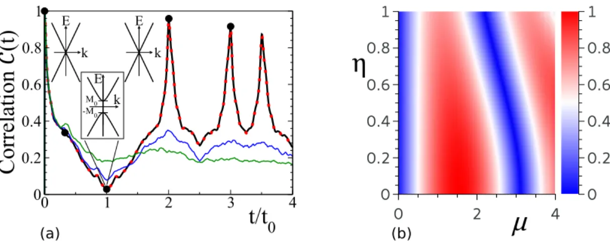
FIG. 2. Quantitative analysis of the echo strength. (a) Correlation C(t), Eq. (4), obtained from numerical propagation of the~-wave, see Fig. 1. Black circles mark the snapshot times. The solid black curve shows distinct echo peaks for the clean Dirac system, Eq. (1). The insets show sketches of the Dirac-type dispersion with a gap opening att=t0. Further curves correspond to different disorder types: gap disorder withτgap ≈0.2t0 (red dotted), spatial disorder withτimp≈0.8t0 (blue) andτimp≈0.2t0 (green). τimp andτgap are the respective elastic scattering times (see Sec. B in the Appendix). (b) Modulus
|A(k)|of the transition amplitude, Eq. (3), plotted as a function of parametersηandµ.
[39] which suggests the QTM to be highly effective in a wide k/energy range. As we will see shortly, the nu- merical simulations confirm this. In general, given an initial wave packetψ(r,0) = (2π)−2R
d2kψ(k,0)eik·r, a convenient measure of the echo strength is given by the correlation
C(t) = Z
d2r|ψ(r,0)||ψ(r, t)| (4) between the moduli of the amplitudes at times 0 andt.
To illustrate the QTM effect, a complicated wave packet resembling ~ is numerically propagated in time (see Fig. 1). At times t0 and 2.5t0, a pulse with M0 = 8hEkiandµ=M0∆t/~=π/2 is applied, with ∆tt0. Here hEki = ahki is the mean wave packet energy, i.e.
hηi = 1/8. The snapshots in Fig. 1 demonstrate that even after full destruction the spatial distribution of the initial wave packet can be reconstructed. This is quanti- fied and confirmed in Fig. 2a), showing the corresponding correlator (4). At the echo time (t= 2t0+∆t≈2t0), ma- jor parts of the time propagated wave packet indeed re- turn to the initial position. This QTM mechanism is not limited to a single pulse: subsequent kicks at t = 2.5t0
and t= 3.25t0 cause further peaks, albeit of decreasing size. The distinct echo peaks, based on the linear disper- sion relation, arise since the kinetic phases accumulated by each k-mode during forward (0→t0) and backward (t0+ ∆t → 2t0+ ∆t) propagation add up to zero (see Appendix A).
The numerical simulations are based on the wave packet propagation algorithm Time-dependent Quantum Transport (TQT) [40]. The state is discretized on a square grid and the time evolution is calculated for suffi- ciently small time steps such that the Hamilton oper- ator can be assumed time independent for each step.
We calculate the action of H on ψ in a mixed posi-
tion and momentum-space representation by the appli- cation of Fourier Transforms. With this a Krylov Space is spanned, which can be used to calculate the time evo- lution using a Lanczos method [41].
For an arbitrary wave packet, the echo strengthC(2t0+
∆t) is analytically given solely in terms of the amplitude A(k), Eq. (3), and the wave packet att= 0 as
C(2t0+∆t) = Z
d2r ψ(r,0)
Z d2k
(2π)2A(k)ψ(k,0)eik·r . (5) Figure 2b) shows the η- and µ-dependence of |A(k)|, obtained from the time-reversal amplitude (3). One finds extended stripes of high fidelity. To check this analytical result we simulate the propagation of a normalized 2D Gaussian wave packet with positive energy and smallk- space width ∆k k0 compared to the absolute value k0 of its mean wave vector, such thatA(k)≈A(k0) for allk-modes involved. Under these assumptions, Eq. (5) reduces toC(2t0+∆t)≈ |A(k0)|(see Appendix A), which can be compared with the correlationC(2t0+∆t), Eq. (4), obtained from full numerical time evolution. As the mean difference between analytics and numerics is 0.03, only the analytical plot is shown. Clearly, strong echoes can be obtained in the full energy range 0.η.1.
III. DISORDER
We now investigate the QTM robustness against dis- order. While this is typically present in a real sys- tem, it should be emphasized that state-of-the-art hBN- encapsulated graphene samples are effectively ballistic over scales of several microns, [42] corresponding to (transport) scattering times of several picoseconds. For the sake of clarity, we keep the discussion at a qualita-
titative details. We consider two types of disorder: a static spatial disorder potential and a spatially random pulse strength (referred to as “gap disorder”). Spatial disorder enters into the Hamiltonian (1) as a time- and (pseudo)spin-independent potentialVimp(r)σ0, whereσ0
is the unit matrix in (pseudo)spin-space. Gap disorder is instead given by Vgap(r)σz fort ∈[t0, t0+ ∆t], i.e.only during the pulse. Both random potentials are Gaussian distributed with width uimp or ugap. As shown in Fig.
2a), the echo is clearly more sensitive to a static ran- dom impurity potential than to gap disorder. This is expected, and can be understood within the framework of Loschmidt echo theory [12, 43, 44]: If a t-inversion protocol is not perfect, the echo signal decays as a func- tion of the propagation timet0. Spatial disorder reduces the fidelity, since the QTM mechanism, even for an op- timally calibrated pulse, achieves “population reversal”
without directly affecting the impurity scattering dynam- ics. In other words, the QTM protocol does not lead to Vimp(r)→ −Vimp(r). In this sense elastic disorder has a qualitatively similar effect to inelastic scattering, whose effects are also not undone by the QTM. Gap disorder plays in principle a similar QTM-breaking role. How- ever, and contrary to spatial disorder, it is active only during the very short pulse duration time ∆t t0 and thus causes only negligible echo losses, reflected in the perfect agreement of the black line and dotted red line in Fig. 2a). Our analysis also highlights a fundamental difference between standard spin echoes and the present wave function echo: while a spin echo decays because of dynamical (inelastic) perturbations leading toT2, the role ofT2is here played by the elastic scattering timeτ.
This suggests an application of the QTM as a probe of the quality of a sample – much as the spin echo is used as a probe of decoherence in two-level systems.
We now explain at a qualitative level how and why static (elastic) disorder affects our echo, whereas spin echoes are insensitive to it. First, consider the scattering off a single impurity, assuming an incoming plane wave with a given propagation direction ˆv. Scattering leads to a position-dependent change of the wave front propaga- tion direction. Considering true time reversal after the scattering process, every scattered part of the wave prop- agates back to the impurity and is scattered again. How- ever, due to destructive interference only the (inverted) initial propagation direction−ˆvsurvives.
In the presence of many scatterers, a Feynman path approach provides convenient insights. While a phase ϕs is accumulated along one particular path s due to scattering off impurities, the same phase with inverted sign −ϕs is picked up on the way back, after (perfect) time inversion due to the time reversal operatorT ∝ Cσy, whereCindicates complex conjugation. Every backward path s0 other than the original one leads to a different phase−ϕs0 6=−ϕs. This causes destructive interference and ensures that only the contribution from the original pathssurvives.
Depending on the environment, the spins precess slower or faster. By applying aπ-pulse at timet0which flips the spin, the faster spins are “suddenly behind” the slower ones. Neglecting inelastic effects, all spins are in phase again at 2t0leading to the Hahn echo [3].
As opposed to the discussion about perfect time rever- sal, our pulse does not define an exact t-inversion pro- tocol even in the absence of inelastic scattering, since it only inverts (“flips”) the kinetic phase due toH0, which is e−iE±t0/~. Without disorder this is the only phase present, and thus it disappears for a closed loop (for- ward, then backward) propagation (see Appendix A).
With disorder the phase due to the random potential Vimp(r) is not inverted and therefore not cancelled after the pulse on the way back. This leads to a “dephasing”, such that contributions from various pathss0 survive at each impurity as opposed to the perfect time reversal dis- cussed above, where only the time-reversed counterpart of the incoming path survives.
IV. CONCLUSIONS
The analytical and numerical considerations presented in this work confirm the principles behind our QTM for pseudo-relativistic graphene-like systems. This means that a sufficiently fast and spatially extended perturba- tion which opens a gap in a Dirac system can act similar to a microwave π pulse in spin-echo experiments, effec- tivelyt-inverting the orbital wave function dynamics and thus generating a wave function echo.
It is important to remark that the QTM does not re- quire time-reversal symmetry to be preserved. Indeed, we checked both analytically and numerically that high- fidelity echoes can also be obtained e.g. in graphene in the presence of a constant perpendicular magnetic field B = ∇ ×A, described by the Hamiltonian H = a[k−(e/~)A]·σ+M(t)σz. Wave packets in this case consist of superpositions of Landau levels with discrete energies En,± ∝ ±√
n [45, 46], while during the pulse the dispersion becomesεn,±=q
M02+En,±2 . The anal- ogy with the discussion of Eq. (1) is evident, and in fact for each electron-like (upper Dirac branch) Lan- dau level, the transition amplitude to its hole-like (lower Dirac branch) equivalent is again given by Eq. (3), where now η =En,±/M0. Since the propagation directions of electron- and hole-like Landau levels are reversed, the QTM principle still applies, and strong echoes are ob- tained for 0.η .1.
The fact that time-reversal invariance need not be pre- served may allow a further twist to the QTM proposal.
The idea is to exploit the orbital effects of a pulsed out-of- plane magnetic field, rather than a mass gap pulse: when the magnetic field is switched on the Dirack-dispersion is abruptly changed to a gapped Landau level spectrum, suggesting the feasibility of a Landau level-based QTM
ture and including the assumption that the inelastic re- laxation time of the injected wave packet is larger than t0. This condition imposes certain restrictions in real graphene [48–50], though femtosecond laser pulses, rou- tinely employed in nano-spectroscopy,[51] could be em- ployed to open gaps therein, and indeed recent experi- mental advances suggest such restrictions not to be crit- ical [52]. On the other hand, certain forms of artificial graphene [34, 36] could be amenable to a straightforward experimental implementation of the QTM. We also note that similar physics can be expected in the surface states of 3D topological insulators,[53] though this will be dis- cussed elsewhere.
We furthermore demonstrated that thet-inversion pro- tocol does not require time-reversal symmetry and is practically insensitive to pulse (gap) disorder. Vice versa, QTM-based echo spectroscopy could be used as a sensi- tive local probe of elastic and inelastic scattering times in Dirac-type systems.
In summary, we have proposed an instantaneous QTM for an extended quantum state, based on the pseudo- relativistic dispersion of (bosonic or fermionic) Dirac-like systems. An experimental realization of such an echo mechanism is within reach in state-of-the-art real or ar- tificial graphene.
ACKNOWLEDGMENTS
We thank R. Huber for useful discussions. A.G.
acknowledges the support of EPSRC Grant No.
EP/K024116/1. C.G., V.K., K.R. and P.R. acknowledge support from Deutsche Forschungsgemeinschaft within SFB 689 and GRK 1570.
Appendix A: Derivation of transition probability to counter-propagating eigenstate
We first derive Eq. (3) describing the transition ampli- tude owing to a time-dependent pulse in a Dirac-type sys- tem. The effective Hamiltonian for graphene-like (single- cone) systems is given by Eqs. (1) and (2). The eigenen- ergies and eigenstates ofH0 are
E±=±ak (A1)
ψ±(k) = 1
√2 1
±e−iθk
, (A2)
where θk is the polar angle in k-space. During the time interval ∆t, an initial H0 eigenstate is subject to Rabi-like oscillations, whose cycle depends on the pulse’s strengthM0 and length ∆t. The new eigenenergies and
χ±(k) = q
a2k2+ (M0+ε±)2
0 ±
ak e−iθk . (A4) Thus, a band gap opens atk= 0 with width ∆ = 2M0.
The time evolution is explicitly performed for one mode, so as to derive the transition probability. Con- sider, an initial eigenstate with negative energy|φk(t = 0)i=|ψ−ki. The indexkis from now on omitted for sake of brevity. The time evolution up tot=t0 is trivial and results in a global phase: |φ(t)i=e−~iE−t0|ψ−i. During the pulse, the time evolution is governed byH, therefore we decompose|ψ−iinto eigenstates|χ±i:
|ψ−i=X
s=±
αs|χsi (A5) with
αs=hχs|ψ−i (A6) and the time evolution fromt =t0 to t =t0+ ∆t =t1 becomes
|φ(t1)i=e−~iE−t0e−~iH∆t|ψ−i
=e−~iE−t0X
s=±
αse−~iεs∆t|χsi. (A7) We are interested only in the component propagating back to its initial position, thus we project|φ(t1)i onto
|ψ+i, which has opposite velocity as compared to the ini- tial state,
hψ+|φ(t1)i=e−~iE−t0X
s=±
αse−~iεs∆thψ+|χsi
=e−~iE−t0X
s=±
αse−~iεs∆tβs∗ (A8) with
βs=hχs|ψ+i. (A9) The component hψ− | φ(t1)i keeps propagating in its initial direction and is lost for the echo.
The echo takes place att= 2t0+ ∆t'2t0(∆tt0), because the absolute value of the velocity is the same for
|ψ+iand |ψ−i. The last propagation step tot2 is again trivial and yields an additional phase e−~iE+t0 for the component traveling back, which cancels with the phase fromt = 0 tot=t0 (E+=−E−). The echo amplitude thus reads
hψ+|φ(t2)i=X
s=±
αsβs∗e−~iεs∆t. (A10)
straightforward but tedious calculation yields hψ+|φ(t2)i=− i
q1 + aM2k22 0
sin M0∆t
~ s
1 +a2k2 M02
!
=− i
p1 +η2sin µp
1 +η2
, (A11)
where the dimensionless parametersη=ak/M0andµ= M0∆t/~ were introduced. Equation (A11) corresponds to Eq. (3). The trivial time evolutions before and after the pulse cancel each other in the absence of disorder, so that the echo strength is solely due to the (modulus of the) transition amplitude to the counter-propagating eigenstate.
Starting in|ψ+iinstead of|ψ−i, or in a superposition of the two, leads to the same conclusions.
For an arbitrary initial wave packet φ(r,0) = (2π)−2R
d2kφ(k,0)eik·r, the simulation-derived echo strength C(2t0) can be analytically estimated. In equa- tions (A5)-(A11), we solve the Schr¨odinger equation ex- actly for the population-reversed part of the wave packet, i.e.the only part contributing to the echo is
φ(k,2t0+ ∆t) =A(k)φ(k,0), (A12) and therefore in real space
φ(r,2t0+ ∆t) =
Z d2k
(2π)2φ(k,2t0)eik·r
=
Z d2k
(2π)2A(k)φ(k,0)eik·r. (A13) As noted, the kinetic phases accumulated before and af- ter the pulse cancel at t = 2t0+ ∆t ' 2t0, preventing interference effects in real space. Moreover, the linear band structure with constant phase velocity keeps the shape of the wave packet.
Thus, our analytical estimate yields C(2t0) =
Z
d2r|φ(r,0)||φ(r,2t0)|
= Z
d2r φ(r,0)
Z d2k
(2π)2A(k)φ(k,0)eik·r
=:CA, (A14)
which is the same as Eq. (5).
In case of nearly constantA(k)≈A(k0), e.g. for nar- row peaked wave packets in k-space around an average valuek0, the echo strength can be estimated by
C(2t0)≈ Z
d2r φ(r,0)
Z d2k
(2π)2A(k0)φ(k,0)eik·r
=A(k0) Z
d2r|φ(r,0)| |φ(r,0)|=A(k0), (A15) having taken a normalized initial wave packet.
1. Spatial disorder
For the numerical investigation of disorder effects, we use a random, pseudospin-independent potential Vimp(r)σ0. The latter assigns to every grid pointia nor- mally distributed valueβi, which is then multiplied with the disorder strengthuimp. The discontinuous potential is then smoothed by a Gaussian distribution with width l0. This leads to
Vimp(r) =uimp
N X
i
βie−
(r−ri)2 l2
0 , (B1)
where the sum runs over all grid points. The normaliza- tionN is due to numerical reasons and is given by
N =
1 A
Z
A
d2r X
i
βie−
(r−ri)2 l2
0
!2
1 2
, (B2)
A being the (finite) grid area for the numerical simula- tion. The correlator
hVimp(r)Vimp(r0)i=u2impe−
(r−r0)2 2l2
0 , (B3)
whereh·istands for disorder average, is needed in order to compute the scattering time. The latter is given by (see e.g. [54])
~ τk
=
Z dk0dr 2π~
δ(k−k0)hVimp(0)Vimp(r)ieir·k0, (B4) and can be calculated analytically as
1 τk
= 2π
a~u2impl20k e−l20k2I0(l20k2). (B5) I0(x) is the modified Bessel function of zeroth kind.
In the main part, we explained on a qualitative level the effect of disorder. Here, we discuss it quantitatively and for that reason we turn to the theory of Loschmidt echoes (see e.g. [43, 44, 55, 56]), where the role of disorder has been thoroughly studied and characterized. In this context the echo is measured by the “fidelity”
M(t) =|hφ|eiHat/~e−iHbt/~|φi|2, (B6) which is the overlap squared between the initial and fi- nal, i.e. time-evolved, state. The time propagation is governed byHb until the timet, and by−Ha thereafter, i.e.the time evolution is (“by hand”) explicitly inverted.
(Note the difference to our protocol where the flow in time is not changed.) Moreover, we use instead the cor- relation C(t), Eq. (4), to quantify the echo in a phys- ically transparent way – as the overlap between initial and time-evolved local density. In order to establish a connection with the Loschmidt echo theory, it is however
0 200 400 600 800 t0 ( /M0)
0.1
echo strength
(a) 0 0.005 uimp(0.01M0) 0.015
0 0.002 0.004 0.006
1/τ0(M0/)
(b)
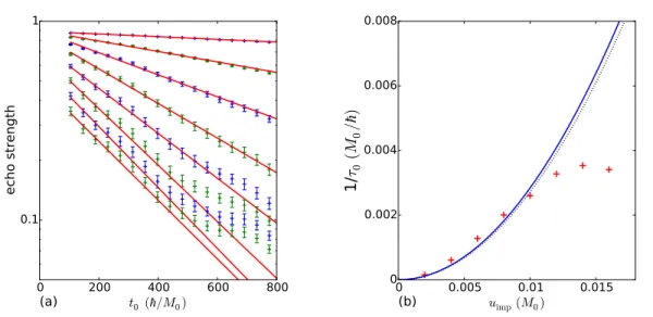
FIG. 3. Effects of disorder on graphene echo. (a) The echo strength measured by the echo fidelity ˜M(techo) is shown as a function of pulse timet0for various disorder strengthsuimpbetween 0.002M0and 0.016M0, averaged over 50 realizations (see text). The error bars denote the standard error of the mean. An exponential fit is used to extract the decay rate. For higher uimp an expected saturation sets in, such that only a brief regime of exponential decay is visible. (b) Plot of the fitted decay rates 1/τ0 as a function of uimp, Eq. (B5), which is quadratic for weak scattering. The black dotted line is the analytically expected curve, which matches well the fitted quadratic function (blue), until the expected strong scattering saturation sets in.
more convenient to introduce the following “echo fidelity”
M˜
M˜(t) =|hσzφ|e−iHt/~|φi|. (B7) Notice the difference with C(t), where |φ| appears, and theσzPauli matrix: ˜M(t) is the overlap of the time prop- agated state with the initial onewith flipped spinor, since the returning part of the wave packet is in the flipped eigenstate of H0. In the golden rule decay regime [44], the (mean) echo strength ˜M decays exponentially in time M˜(t)∼e−2τt . (B8) As mentioned, the pulse time-reverses the dynamics due to H0 only, without affecting the dynamics arising from the impurity potential.
This can be seen by splitting the time evolution op- erator in three parts: before the pulse, during the pulse and after the pulse. Furthermore, we consider only the part of the wave function which is reflected, which means that the time evolution during the pulse is given by the transition amplitude A(k) times the operator σz, which maps any state to its energy-inversed counterpart.
M˜(2t0) =|hφ|σze−i~(H0+Vr)t0σzA(k)e−~i(H0+Vr)t0|φi|2
=|hφ|e−~iσz(H0+Vr)σzt0A(k)e−~i(H0+Vr)t0 |φi|2 (B9) Since σzσiσz = −σi for i ∈ {x, y} and H0 is a lin- ear combination of σx and σy, the sign in front of H0
changes after the pulse, whereas the term related to the
pseudospin-independent potentialVris not affected at all by the pulse.
M˜(2t0) =|hφ|e−~i(−H0+Vr)t0A(k)e−~i(H0+Vr)t0 |φi|2. (B10) As there is a different sign in the propagation due toH0 before and after the pulse, there iseffectivelya propaga- tion backwards in time. On the other hand, ourσz-pulse cannot invert the time evolution due to the disorder po- tential, which causes disorder to ultimately destroy the echo.
Since the scattering occurs during the whole propaga- tion time 2t0, we expect the echo fidelity (B8) to decay as
M˜(2t0)∼e−2t2τ0 =e−tτ0. (B11) This decay is confirmed in Fig. 3a), where the echo fi- delity (= echo strength), Eq. (B7), is shown as a function of the pulse time t0. The initial wave packet is a 2D- Gaussian with smallk-space widthσk k0as compared to the mean wave vectork0, such that thek-dependence of the scattering time can be neglected (τk ≈τk0 =:τ0).
The echo strength is calculated for 50 different realiza- tions of the random disorder potential and averaged sub- sequently. For large disorder strengthsuimp, a saturation regime is reached, in accordance with Loschmidt echo theory[44]. The decay rate is extracted by fitting an ex- ponentially decaying function to the data, and compared in Fig. 3b) to the analytically expected decay rate 1/τ0
from Eq. (B5), yielding a good agreement.
slower, because the phase differences between the ini- tial and the propagated wave packet are neglected in the modulus, preventing eventual destructive interference.
2. Gap disorder
The gap disorder potentialVgap(r)σz models fluctua- tions in the pulse strength and is therefore only active in the short time window ∆t. Figure 2 a) shows that gap
pared to spatial disorder. This is expected, as spatial disorder is active during a time 2t0 ∆t. Assuming similar scattering times foruimp = ugap, practically no gap disorder-induced scattering takes place during the pulse, sinceτ0∆t. Moreover, spatial and gap disorder acts slightly differently. The impurities lead to a random- ization of the propagation direction, such that a smaller amount of the wave packet goes back to the initial posi- tion. Gap disorder instead modulates in space the tran- sition probability to the counter-propagating eigenstate, but the propagation direction is not randomized.
[1] J. Loschmidt, “ ¨Uber den Zustand des W¨armegleichgewichts eines Systems von K¨orpern mit R¨ucksicht auf die Schwerkraft,” Sitzungberichte der Akademie der WissenschaftenII, 128 (1876).
[2] L. Boltzmann, “ ¨Uber die Beziehung eines allgemeinen mechanischen Satzes zum zweiten Hauptsatze der W¨armetheorie,” Sitzungberichte der Akademie der Wis- senschaftenII, 67 (1877).
[3] E. L. Hahn, “Spin echoes,” Phys. Rev.80, 580 (1950).
[4] J. A. Weil and J. R. Bolton,Electron Paramagnetic Res- onance (John Wiley & Sons, 2007).
[5] M. Fink, “Time reversal of ultrasonic fields. I. Basic prin- ciples,” Ultrasonics, Ferroelectrics, and Frequency Con- trol, IEEE Transactions on39, 555–566 (1992).
[6] C. Draeger and M. Fink, “One-channel time reversal of elastic waves in a chaotic 2d-silicon cavity,” Phys. Rev.
Lett.79, 407 (1997).
[7] M. Fink, “Time reversed acoustics,” Physics Today 50, 34 (1997).
[8] G. Lerosey, J. de Rosny, A. Tourin, A. Derode, G. Mon- taldo, and M. Fink, “Time reversal of electromagnetic waves,” Phys. Rev. Lett.92, 193904 (2004).
[9] A. Przadka, S. Feat, P. Petitjeans, V. Pagneux, A. Mau- rel, and M. Fink, “Time reversal of water waves,” Phys.
Rev. Lett. 109, 064501 (2012).
[10] A. Chabchoub and M. Fink, “Time-reversal generation of rogue waves,” Phys. Rev. Lett.112, 124101 (2014).
[11] H. M. Pastawski, E. P. Danieli, H. L. Calvo, and L. E.
F. Foa Torres, “Towards a time reversal mirror for quan- tum systems,” EPL77, 40001 (2007).
[12] H. L. Calvo, R. A. Jalabert, and H. M. Pastawski, “Semi- classical theory of time-reversal focusing,” Phys. Rev.
Lett.101, 240403 (2008).
[13] H. L. Calvo and H. M. Pastawski, “Exact time-reversal focusing of acoustic and quantum excitations in open cav- ities: The perfect inverse filter,” EPL89, 60002 (2010).
[14] A. P. Mosk, A. Lagendijk, G. Lerosey, and M. Fink,
“Controlling waves in space and time for imaging and focusing in complex media,” Nat. Phot.6, 283 (2012).
[15] A. Yariv, “Four wave nonlinear optical mixing as real time holography,” Opt. Commun.25, 23–25 (1978).
[16] D. A. B. Miller, “Time reversal of optical pulses by four- wave mixing,” Opt. Lett.5, 300–302 (1980).
[17] M. Moshinsky, “Diffraction in time,” Phys. Rev.88, 625 (1952).
[18] A. S. Gerasimov and M. V. Kazarnovskii, “Possibility of observing nonstationary quantum-mechanical effects by means of ultracold neutrons,” Sov. Phys. JETP44, 892 (1976).
[19] ˇC. Brukner and A. Zeilinger, “Diffraction of matter waves in space and in time,” Phys. Rev. A56, 3804 (1997).
[20] J. T. Mendon¸ca and P. K. Shukla, “Time refraction and time reflection: Two basic concepts,” Phys. Scripta65, 160 (2002).
[21] A. del Campo, G. Garcia-Calder´on, and J. G. Muga,
“Quantum transients,” Phys. Rep.476, 1 (2009).
[22] A. Goussev, “Huygens-Fresnel-Kirchhoff construction for quantum propagators with application to diffraction in space and time,” Phys. Rev. A85, 013626 (2012).
[23] P. Haslinger, N. Dorre, P. Geyer, J. Rodewald, S. Nimm- richter, and M. Arndt, “A universal matter-wave inter- ferometer with optical ionization gratings in the time do- main,” Nat. Phys.9, 144 (2013).
[24] J. Martin, B. Georgeot, and D. L. Shepelyansky, “Cool- ing by time reversal of atomic matter waves,” Phys. Rev.
Lett.100, 044106 (2008).
[25] J. Martin, B. Georgeot, and D. L. Shepelyansky, “Time reversal of Bose-Einstein condensates,” Phys. Rev. Lett.
101, 074102 (2008).
[26] A. Ullah and M. D. Hoogerland, “Experimental obser- vation of loschmidt time reversal of a quantum chaotic system,” Phys. Rev. E83, 046218 (2011).
[27] Y. Sivan and J. B. Pendry, “Time reversal in dynamically tuned zero-gap periodic systems,” Phys. Rev. Lett.106, 193902 (2011).
[28] Y. Sivan and J. B. Pendry, “Theory of wave-front reversal of short pulses in dynamically tuned zero-gap periodic systems,” Phys. Rev. A84, 033822 (2011).
[29] V. Bacot, M. Labousse, A. Eddi, M. Fink, and E. Fort,
“Time reversal and holography with spacetime trans- formations,” Nat. Phys. (advance online publication) (2016), 10.1038/nphys3810.
[30] Video available at Regensburg library.
[31] E. Bocquillon, V. Freulon, F. D. Parmentier, J.-M.
Berroir, B. Pla¸cais, C. Wahl, J. Rech, T. Jonckheere, T. Martin, C. Grenier, D. Ferraro, P. Degiovanni, and G. F`eve, “Electron quantum optics in ballistic chiral con- ductors,” Ann. Phys. (Berlin)526, 1 (2013).
[32] T. Jullien, P. Roulleau, B. Roche, A. Cavanna, Y. Jin, and D. C. Glattli, “Quantum tomography of an electron,”
Nature514, 603 (2014).