Research Collection
Working Paper
Performance guarantees of forward and reverse greedy
algorithms for minimizing nonsupermodular nonsubmodular functions on a matroid
Author(s):
Karaca, Orçun; Tihanyi, Dániel; Kamgarpour, Maryam Publication Date:
2021
Permanent Link:
https://doi.org/10.3929/ethz-b-000471342
Rights / License:
In Copyright - Non-Commercial Use Permitted
This page was generated automatically upon download from the ETH Zurich Research Collection. For more information please consult the Terms of use.
ETH Library
Performance guarantees of forward and reverse greedy algorithms for minimizing nonsupermodular nonsubmodular functions on a matroid
Orcun Karacaa,∗, Daniel Tihanyia, Maryam Kamgarpourb
aAutomatic Control Laboratory, D-ITET, ETH Z¨urich, Switzerland
bElectrical and Computer Engineering Department, University of British Columbia, Vancouver, Canada
Abstract
This letter studies the problem of minimizing increasing set functions, or equivalently, maximizing decreasing set functions, over the base of a matroid. This setting has received great interest, since it generalizes several applied problems including actuator and sensor placement problems in control theory, multi-robot task allocation problems, video summarization, and many others. We study two greedy heuristics, namely, the forward and the reverse greedy algorithms. We provide two novel performance guarantees for the approximate solutions obtained by these heuristics depending on both the submodularity ratio and the curvature.
Keywords: Combinatorial optimization, Greedy algorithm, Matroid theory
1. Introduction
Set function optimization is an active field of research which is used in a broad range of appli- cations including video summarization in machine learning [1, 2], splice site detection in computa- tional biology [3, 2], actuator and sensor placement problems in control theory [4–8], multi-robot task allocation problems in robotics [9–14] and many others. In this letter, we study the following case: the problem of minimizing an increasing nonsubmodular and nonsupermodular set function (or equivalently, maximizing a decreasing set function) over the base of a matroid. The objective and the constraints of this problem are general enough to model many of these application instances for which NP-hardness results are available in the literature [15]. Thus, it is desirable to obtain scalable algorithms with provable suboptimality bounds.
Many studies have adopted greedy heuristics, because of their polynomial-time complexity and the performance bounds they are equipped with [16–19]. For the forward greedy algorithm applied to our setting, [19, Theorem 7] provides a performance guarantee based on the notion ofstrong1
∗Corresponding author
Email addresses: okaraca@ethz.ch(Orcun Karaca),tihanyid@ethz.ch(Daniel Tihanyi), maryamk@ece.ubc.ca(Maryam Kamgarpour)
1We use the term strong curvature to differentiate between the definition of curvature from [19] and the definitions in our work and in [1].
curvature, describing how modular the objective is. As an alternative, [7, Theorem 2] provides a guarantee based on the weaker notions of submodularity ratio (describing how submodular the ob- jective is) and curvature (describing how supermodular the objective is). However, this guarantee scales with the cardinality of the ground set. To the best of our knowledge, there exists no for- ward greedy guarantee applicable to our setting utilizing both submodularity ratio and curvature, simultaneously, which is also problem-size independent. This will be the first goal of this letter.
An inherent drawback of the forward greedy algorithm is that any performance guarantee has to involve the objective evaluated at the empty set as the reference value. This reference is known to have an undesirable effect in several applications [20–22, 7]. An alternative is to adopt the reverse greedy, which excludes the least desirable elements iteratively starting from the full set.
In this case, any potential performance guarantee would instead involve the objective function evaluated at the full set, which might be a more preferable reference point. For the reverse greedy applied to our setting, [19, Theorem 6] provides a performance guarantee again based on the notion of strong curvature. When only cardinality constraints are present, [1, Theorem 1] is applicable and it provides a guarantee based on the weaker notions of submodularity ratio and curvature.
However, to the best of our knowledge, there exists no reverse greedy guarantee applicable to our setting utilizing both curvature and submodularity ratio, simultaneously. This will be the second goal of this letter.
Our contributions are as follows. We obtain a performance guarantee for the forward greedy algorithm applied to minimizing increasing nonsubmodular and nonsupermodular set functions, characterized by submodularity ratio and curvature, over the base of a matroid. This result is presented in Theorem 1. For the same setting, we then obtain a performance guarantee for the reverse greedy algorithm, see Theorem 2. Both guarantees utilize a version of the ordering property derived in [23, Lemma 1], which is inspired by its continuous polymatroid counterpart from [18, Theorem 6.1]. For both guarantees, we demonstrate more efficient greedy notions of the curvature and the submodularity ratio, since the original definitions are computationally intractable. Finally, we provide a comparison of these two theoretical performance guarantees for different values of submodularity ratio and curvature.
In the remainder, Section 2 introduces preliminaries and problem formulation. Sections 3.1 and 3.2 study the forward and the reverse greedy algorithms, respectively, and derive guarantees.
Section 4 presents the comparison.
2. Preliminaries
2.1. Properties of set functions and set constraints
We introduce well-studied notions from combinatorial optimization literature [24–27].
LetV be a finite ground set andf : 2V →Rbe our set function. In literature, function is called normalized whenever f(∅) = 0, however, assume this is not necessarily the case. For notational
simplicity, we usej and {j}interchangeably for singleton sets.
Definition 1. Function f is increasing if f(S)≤f(R),for all S ⊆R⊆V. Function −f is then decreasing. If the inequality is strict whenever S ( R, then f is strictly increasing and −f is strictly decreasing.
Definition 2. For any S ⊆V and j ∈V, discrete derivative of f at S with respect to j is given by ρj(S) =f(S∪j)−f(S).
If j ∈ S, we have ρj(S) = 0. For any R ⊆V, we generalize the definition above to ρR(S) = f(S∪R)−f(S).
Definition 3. Function f is submodular if ρj(R)≤ρj(S),for all S⊆R⊆V, for allj ∈V \R.
In several practical problems, the discrete derivative diminishes as S expands yielding the submodularity property, see the examples in [28, 29]. Unfortunately, functions used in many problems, including the ones we consider, do not have this property. Instead, these problems involve increasing set functions, allowing the use ofsubmodularity ratiodescribing how far a nonsubmodular set function is from being submodular. This property was first introduced by [30].
Definition 4. The submodularity ratio of an increasing function f is the largest scalar γ ∈ R+
such that γρj(R) ≤ρj(S), for all S ⊆ R ⊆V, for all j ∈V \R. Function f with submodularity ratio γ is called γ-submodular.
Observe that the definition above is not well-posed unlessf is increasing, in other words, both ρj(R) andρj(S) are nonnegative.2 It can easily be verified that, for an increasing functionf, we haveγ ∈[0,1] and submodularity is attained if and only ifγ = 1.
We briefly review an alternative but nonequivalent submodularity ratio notion from [1, 31]. The cumulative submodularity ratio is the largest scalar γ0 ∈ R+ such that γ0ρR(S) ≤P
j∈R\Sρj(S), for allS, R⊆V. The ratioγ of Definition 4 satisfies the inequalities for the definition ofγ0, but the reverse argument does not necessarily hold. Hence,γ ≤γ0, see [7, Appendix B]. This notionγ0 is generally restricted to the case when deriving guarantees for greedy heuristics with only cardinality constraints, because only then it allows to derive bounds of the form of [1, Lemma 1] for the linear programming proof from [18]. Utilizing the submodularity notion as per Definition 4 is needed for the guarantees we will derive.
Definition 5. Function f is supermodular ifρj(R)≥ρj(S),for all S ⊆R⊆V, for all j∈V \R.
2Functionf is submodular, if and only if−f is supermodular. Thus, one may consider the submodularity ratio of a decreasing functionf to be the curvature of−f, see Definition 6 below.
Other than submodularity, another widely-used notion is supermodularity we defined above, that is, the increasing discrete derivatives property. A function which is both supermodular and submodular is modular/additive. Similar to the case with submodularity, objective functions we consider do not exhibit supermodularity as well. By introducing the curvature, that is, how far a nonsupermodular increasing function is from being supermodular, we obtain a more precise description on how the discrete derivatives change.
Definition 6. The curvature of an increasing function f is the smallest scalar α ∈R+ such that ρj(R)≥(1−α)ρj(S),for all S⊆R ⊆V, for all j ∈V \R. Function f with curvature α is called α-supermodular.
It can easily be verified that, for an increasing functionf, we haveα∈[0,1] and supermodularity is attained if and only if α = 0. A cumulative definition is also applicable, however, we leave it out, see [32].
Next, we provide two propositions regarding these ratios. The first is an observation relevant for the applications from the literature we discuss. The second will be useful when adopting the reverse greedy algorithm.
Proposition 1. Suppose f is strictly increasing and 0 < f ≤ ρj(S) ≤ f , for all S ( V, for all j /∈S. Then, we haveγ ≥f
f andα≤1−f f.
Proof. Since ρj(R) > 0, by reorganizing Definition 4, we obtain γ = minS⊆R⊆V, j∈V\Rρj(S) ρj(R). Clearly, the term on the right is lower bounded by f
f. Similarly, we can reorganize Definition 6 as follows 1
(1−α) = maxS⊆R⊆V, j∈V\R ρj(S)
ρj(R). The term on the right is upper bounded by f f . A simple manipulation of the inequality gives us the desired result.
Proposition 2. Let fˆ(S) =−f(V \S),for all S⊆V.Let γˆ andαˆ be the submodularity ratio and the curvature of functionfˆ, respectively. Then, we have ˆγ = 1−α andαˆ= 1−γ.
Proof. Observe that function fˆis increasing, hence submodularity ratio and curvature are well- defined. Let ρˆj(S) = ˆf(S∪j)−fˆ(S) =f(V \S)−f({V \S} \j}),for all S, j. The submodularity ratio of function fˆis the largest scalar γˆ such that γˆρˆj(R) ≤ ρˆj(S), for all S ⊆ R ⊆ V, for all j∈V\R. Using the definition ofρˆj, this ratio is also the largest scalarˆγ such thatγρˆ j(S)≤ρj(R), for allS ⊆R⊆V, for all j∈V \R. Thus, ˆγ = 1−α by Definition 6. Using a similar reasoning,
one would also obtainαˆ= 1−γ.
Many combinatorial optimization problems from the literature are subject to constraints that are more complex than simple cardinality constraints, see the examples in [33, 34]. Among those, we introduce matroids. They will capture problems of interest in Section 2.2. Moreover, they are known to allow performance guarantees for greedy heuristics thanks to their specific properties outlined below [35, 36].
Definition 7. A matroidMis an ordered pair(V,F)consisting of a ground setV and a collection F of subsets of V which satisfies
(i) ∅ ∈ F,
(ii) if S, R∈ F andR (S, then R∈ F,
(iii) if S1,S2∈ F and |S1|<|S2|, there exists j∈S2\S1 such that j∪S1 ∈ F.
Every set in F is called independent. Maximum independent sets refer to those with the largest cardinality, and they are called the bases of a matroid.
Clearly, all bases have the same cardinality by property(iii). This last property of a matroid is considered as the generalization of the linear independence relation from linear algebra. Intuitively, this property will later let us to keep track of the elements that the greedy algorithm is missing from the optimal solution.
To adopt the reverse greedy algorithm, an additional concept will be required, that is, the dual of a matroid.
Definition 8. Given a matroidM= (V,F), letFˆ ={U | ∃ a baseM ∈ F such that U ⊆V\M}.
The pair Mˆ = (V,Fˆ) is called the dual of the matroid (V,F).
The pair ˆM= (V,F) satisfies all the axioms of a matroid. Supposeˆ {Mi}qi=1 is the collection of all bases of matroid (V,F). Then, {V \Mi}qi=1 defines the collection of all bases for the dual (V,F), see [27, Ch. 2] and [7, Lemma 1].ˆ
2.2. Problem formulation Our goal is to solve
S⊆Vmin f(S), increasing,γ-submodular, α-supermodular s.t. S∈ F, M= (V,F) is a matroid,|S|=N,
(1)
where the cardinality of any base of M is given by N ∈ Z+. The guarantees we derive will be applicable as long as the cardinality of any base ofMis larger than or equal toN. Note that if not, the problem would be infeasible. We can reformulate such problems as (1), since the intersection of a uniform matroid (i.e.,{S ⊆V | |S| ≤Q},whereQ∈Z+, Q≤ |V|) and any matroid results in another matroid. Finally, let S∗ denote the optimal solution of (1).
Let us briefly explain three of the well-studied applications the problem above can model.
•In multi-robot task allocation, the goal is to distribute a given set of tasks to a fleet of robots.
The ground set V is the set of all robot-task pairs, and the constraints are given by a partition matroid and a cardinality constraint. The objective is a measure defined over the set partitions.
For instance, in [13], the goal is to maximize the success probability of a mission which decreases
when more and more tasks are allocated to the robots. This measure is both nonsubmodular and nonsupermodular. Observe that such problems can equivalently be stated as the minimization of an increasing function as in (1).
• In actuator placement problem, the goal is to select a subset from a finite set of possible placements when designing controllers over a large-scale network. The ground setV is the set of all possible placements. The constraints can be a cardinality constraint on the number of actuators, and also a controllability requirement (a matching matroid). The objective is then a desired network performance metric. For instance, in [7], the goal is to minimize an energy consumption metric, which increases as we pick more and more actuators to remove from the network (the so-called actuator removal problem). Thus, this problem maps to (1). Such metrics are well-known to be nonsubmodular and nonsupermodular, and the literature obtains bounds on the submodularity ratio and the curvature based on versions of Proposition 1 utilizing eigenvalue inequalities, see [37, Propositions 1 and 2].
•In video summarization, the goal is to to pick a few frames from a video which summarize it.
The ground setV is the set of all frames, and the constraints are both a cardinality constraint and a partition constraint, for instance, to extract one representative frame from every minute. The objective is a summary quality measure defined over a set of frames. For instance, in [2], the goal is to maximize an objective that favors subsets with higher diversity. This problem can easily be reformulated such that it maps to (1).
3. Greedy algorithms
3.1. Forward greedy algorithm and the performance guarantee
For Algorithm 1, the following definitions and explanations are in order. At iteration t, the forward greedy algorithm choosesst:=St\St−1 with the corresponding discrete derivative ρt:=
f(St)−f(St−1). In Line 5, we have a matroid feasibility check. We assume that this can be done in polynomial-time, which is the case for all the applications we discussed above, e.g., [7,§5.B&C].
Thanks to the properties of a matroid, we do not need to reconsider an element that has already been rejected by the feasibility check. To this end, the set Ut denotes the set of elements having been considered by the matroid feasibility check before choosing st+1. The final forward greedy solution is Sf := SN, and it is a base of (V,F), since it lies in F and has cardinality N by the properties of a matroid.
Main result is shown in the following theorem.
Theorem 1. If Algorithm 1 is applied to (1), then f(Sf)−f(∅)
f(S∗)−f(∅) ≤ 1
γ(1−α). (2)
We first need the following lemma.
Algorithm 1 Forward Greedy Algorithm
Input: Set functionf, ground setV, matroid (V,F), cardinality constraintN Output: Forward greedy solution Sf
1: functionForwardGreedy(f, V,F, N)
2: S0 =∅,U0 =∅,t= 1
3: while |St−1|< N do
4: j∗(t) = arg minj∈V\Ut−1ρj(St−1)
5: if St−1∪j∗(t)∈ F/ then
6: Ut−1←Ut−1∪j∗(t)
7: else
8: ρt←ρj∗(t)(St−1) and st=j∗(t)
9: St←St−1∪j∗(t) andUt←Ut−1∪j∗(t)
10: t←t+ 1
11: end if
12: end while
13: Sf ←SN
14: end function
Lemma 1. For any base M ∈ F, the elements of M ={m1, . . . , mN} can be ordered so that ρmt(St−1)≥ρt=ρst(St−1),
holds for t= 1, . . . , N.Moreover, whenever st∈M, we have that mt=st.
Proof. For this proof, we extend a method from a similar ordering property which is derived when applying greedy heuristics on dependence systems [23, Lemma 1] (specifically on comatroids, which are the complementary notion of matroids in independence systems, see also [24, 38, 39]). [23, Lemma 1] was originally inspired by a study on greedy heuristics over integral polymatroids (that is, a continuous extension of matroids), see [18, Theorem 6.1].
We prove by induction. Assume the elements {mt+1, . . . , mN} are found. Let M˜t = M \ {mt+1, . . . , mN}. If st ∈ M˜t, we let mt = st, and the condition is satisfied, and the second statement of the lemma holds. If st 6∈M˜t, by property (iii) of Definition 7 and M˜t∈ F, we know that there exists j ∈ M˜t\St−1 such that j∪St−1 ∈ F. Moreover, ρj(St−1) ≥ ρst(St−1), since j is not the element chosen by the greedy algorithm. Hence, we pick mt =j. The existence of mN
follows from property (iii) of Definition 7: there existsmN ∈M\SN−1 such thatmN∪SN−1∈ F.
This concludes the proof.
This lemma plays a significant role in obtaining suboptimality bounds, which becomes clear once we pick M to be the optimal solutionS∗ in the following proof of Theorem 1.
Proof (Proof of Theorem 1). LetS∗ ={s∗1, . . . , s∗N}, where the elements s∗t are ordered accord- ing to Lemma 1. Let St∗ = {s∗1, . . . , s∗t} for t = 1, . . . , N, and S0∗ = ∅. Using this definition, we obtain
f(S∗)−f(∅) =
N
X
t=1
ρs∗
t(S∗t−1)≥(1−α)
N
X
t=1
ρs∗t(∅). (3)
The equality follows from a telescoping sum. The inequality follows from Definition 6. On the other hand, a similar observation can also be made for the forward greedy solution as follows
f(Sf)−f(∅) =
N
X
t=1
ρt
= X
t:st∈S∗
ρst(St−1) + X
t:st∈S/ ∗
ρst(St−1),
where the last equality decomposes the greedy steps into those that coincide with the optimal solution and those that do not. Invoking Lemma 1 for the term on the right-hand side, we obtain
f(Sf)−f(∅)≤ X
t:st∈S∗
ρst(St−1) + X
t:s∗t∈S/ f
ρs∗
t(St−1), (4)
where the term on the right also utilizes {t :st ∈/ S∗} = {t: s∗t ∈/ Sf}, which is a direct result of the last statement of Lemma 1. Now, notice that for any s∗t ∈/ Sf we have s∗t ∈/ St−1. Hence using Definition 4, we obtain
f(Sf)−f(∅)≤ X
t:st∈S∗
ρst(St−1) +1 γ
X
t:s∗t∈S/ f
ρs∗t(∅).
Next, the term on the left can also be upper bounded by utilizing Definition 4, giving us
f(Sf)−f(∅)≤ 1 γ
X
t:st∈S∗
ρst(∅) + 1 γ
X
t:s∗t∈S/ f
ρs∗t(∅)
= 1 γ
X
t:st∈S∗
ρst(∅) + 1 γ
X
t:st∈S/ ∗
ρs∗
t(∅)
= 1 γ
N
X
t=1
ρs∗
t(∅),
(5)
The first equality reapplies the set reformulation {t:st∈/ S∗}={t:s∗t ∈/ Sf} (previously found in (4)), and the second equality combines the two summations. Finally, we can combine (3) and (5), to obtain
f(Sf)−f(∅)
f(S∗)−f(∅) ≤ 1 γ(1−α).
This completes the proof of theorem.
[7, Theorem 2] offers a guarantee for this setting. This is given by 1−γγ (2N+ 1)
1−γ γ(1−α) −1
.In contrast, the guarantee in Theorem 1 above is independent of the problem size, and also tighter for any of the (α, γ, N) pairs.3
3[7, Propositions 4 and 5] prove that there is no performance guarantee for the forward greedy algorithm unless both submodular-like and supermodular-like properties are present in the objective function. Observe that this is confirmed by Theorem 1.
As an alternative, [19, Theorem 7] offers another guarantee, which is given by 1/(1−c), where the strong curvaturecquantifies how far a function is from being modular: the smallest parameter c∈[0,1] such thatρj(R) ≥(1−c)ρj(S),for all S, R⊆V \j. This novel notion is a significantly stronger requirement than having both the submodularity ratio and the curvature, simultane- ously [7]. Hence, it is not possible to compare it with our guarantee other than the case of a modular objective, that is, c = 0, γ = 1, α = 0. For both guarantees, modularity confirms the optimality of the forward greedy algorithm, as it is well-established by the Rado-Edmonds theo- rem [36]. Note that computing the strong curvature notion requires an exhaustive enumeration of all inequalities in its definition, since the proof method of [19, Theorem 7] does not allow any greedy curvature computation as we present below.
Corollary 1. Let γfg be the largest ˜γ that satisfiesγρ˜ s(S)≤ρs(∅) for all S∈ F, |S| ≤N−1 and S∪s∈ F. Then, γfg is called the forward greedy submodularity ratio with γfg ≥γ. Let αfg be the smallest α˜ that satisfies ρs(S) ≥(1−α)ρ˜ s(∅) for all S ∈ F, |S| ≤ N −1 and S∪s∈ F. Then, αfg is called the forward greedy curvature with αfg ≤ α. The performance guarantee can then be written as
f(Sf)−f(∅)
f(S∗)−f(∅) ≤ 1
γfg(1−αfg),or equivalently, f(Sf)≤ 1
γfg(1−αfg)f(S∗) + 1− 1 γfg(1−αfg)
! f(∅).
The forward greedy submodularity ratio and the forward greedy curvature can be obtained in an ex-post manner after the algorithm is completed. For each of these notions, we need to analyze O( |VN|
) inequalities, which could still be large, but they are significantly more tractable than the original definitions. Since γfg ≥ γ and αfg ≤ α, the performance guarantee in Corollary 1 can essentially be better than the one in Theorem 1. Notice that (γfg, αfg) changes with the constraint set of the problem since the inequalities defining (γfg, αfg) would then be different. In contrast, submodularity ratio and curvature depend only on the objective function.
The performance guarantee in Corollary 1 can still be loose, because of the reference valuef(∅).
For instance, in multi-robot task allocation problems,f(∅) corresponds to minus the safety of a plan with no tasks, see [13]. In such applications, the values f(∅) ≈ −1 and (1−1/[γfg(1−αfg)]) <0 can make the bound in (1) large.
In the next section, we consider a variant of the greedy algorithm that comes along with a performance guarantee that does not depend on f(∅).
3.2. Reverse greedy algorithm and the performance guarantee
For Algorithm 2, the following definitions and explanations are in order. For compactness, we define a shifted discrete derivative δj(S) := ρj(S \j) = f(S)−f(S \j), for all S ⊆ V, j ∈ S.
At iterationt, the reverse greedy algorithm chooses rt:=Xt−1\Xt to remove, with the maximal
Algorithm 2 Reverse Greedy Algorithm
Input: Set functionf, ground setV, matroid (V,F), cardinality constraintN Output: Reverse greedy solution Sr
1: functionReverseGreedy(f, V,F, N)
2: X0 =V,Y0 =∅,t= 1
3: while |Xt−1|> N do
4: k∗(t) = arg maxj∈V\Yt−1δj(Xt−1)
5: if ∃M ∈ F such that M ⊆
Xt−1\k∗(t) and |M|=N then
6: Yt−1←Yt−1∪k∗(t)
7: else
8: δt←δk∗(t)(Xt−1) and rt=k∗(t)
9: Xt←Xt−1\k∗(t) and Yt←Yt−1∪k∗(t)
10: t←t+ 1
11: end if
12: end while
13: Sr ←X|V|−N
14: end function
reduction δt := f(Xt−1)−f(Xt). In Line 5, we have a matroid feasibility check. In contrast to Algorithm 1, this matroid feasibility check requires that our intermediate solutions are supersets of a base of the matroidM.The setYt denotes the set of elements having been considered by the matroid feasibility check before choosing xt+1. The final reverse greedy solution isSr :=X|V|−N, and it is a base of (V,F), since it lies inF and has cardinalityN by the properties of a matroid.
Main result is shown in the following theorem.
Theorem 2. If Algorithm 2 is applied to (1), then f(V)−f(Sr)
f(V)−f(S∗) ≥ 1−α
1 + (1−γ)(1−α).
For the sake of clarity of the notation, our proof will utilize the following reformulation of (1):
maxR⊆V
fˆ(R) :=−f(V \R), increasing, (1−α)-submodular, (1−γ)-supermodular s.t. R∈Fˆ, Mˆ = (V,F) is a matroid,|R|=|V| −N = ˆN ,
(6)
where the cardinality of any base of ˆM is given by |V| −N = ˆN ∈ Z+. The equivalence of (1) and (6) follows directly from Proposition 2 and Definition 8 (that is, the definition of the dual matroid). Denote its optimal solution byR∗. Clearly, we haveR∗=V \S∗.
Forward greedy algorithm applied to (6) is presented in Algorithm 3, where we define ˆρj(R) = fˆ(R∪j)−fˆ(R), for all R⊆V and j ∈V. Iterations of this algorithm coincide with those of the reverse greedy algorithm applied to (1). Denote the forward greedy iterates byRt.At any iteration, we have Xt= V \Rt. At iteration t, the forward greedy algorithm chooses rt := Rt\Rt−1 with
Algorithm 3 Forward Greedy Reformulation of Reverse Greedy Algorithm
Input: Set function ˆf, ground setV, dual matroid (V,F), cardinality constraint ˆˆ N Output: Reverse greedy solution Sr
1: functionReverseGreedyReformulated(f, V,F,ˆ Nˆ)
2: R0=∅,Y0 =∅,t= 1
3: while |Rt−1|<Nˆ do
4: k∗(t) = arg maxj∈V\Yt−1ρˆj(Rt−1)
5: if Rt−1∪k∗(t)∈/ Fˆ then
6: Yt−1←Yt−1∪k∗(t)
7: else
8: ρˆt←ρˆk∗(t)(Rt−1) and rt=k∗(t)
9: Rt←Rt−1∪k∗(t) and Yt←Yt−1∪k∗(t)
10: t←t+ 1
11: end if
12: end while
13: Sr ←V \RNˆ
14: end function
the corresponding discrete derivative ˆρt:= ˆf(St)−fˆ(St−1).
With the observations above in mind, we bring the ordering lemma.
Lemma 2. For any base M ∈F, the elements ofˆ M ={m1, . . . , mNˆ} can be ordered so that ˆ
ρmt(Rt−1)≤ρˆt= ˆρrt(Rt−1),
holds for t= 1, . . . ,N .ˆ Moreover, whenever rt∈M, we have that mt=rt.
Proof. The proof is a reformulation of that of Lemma 1, by changing the greedy minimization to a greedy maximization. We prove by induction. Assume the elements {mt+1, . . . , mNˆ} are found.
Let M˜t=M\ {mt+1, . . . , mNˆ}. If rt∈M˜t, we let mt =rt, and the condition is satisfied, and the second statement of the lemma holds. Ifrt6∈M˜t, by property (iii) of Definition 7 andM˜t∈F, weˆ know that there existsj∈M˜t\Rt−1 such thatj∪Rt−1 ∈ F. Moreover,ρˆj(Rt−1)≤ρˆrt(Rt−1), since j is not the element chosen by the greedy algorithm. Hence, we pick mt=j. The existence of mNˆ
follows from property (iii) of Definition 7: there existsmNˆ ∈M\RN−1ˆ such that mNˆ∪RNˆ−1∈F.ˆ
This concludes the proof.
We are now ready to prove our theorem.
Proof (Proof of Theorem 2). LetR∗ ={r∗1, . . . , r∗ˆ
N}, where the elementsrt∗ are ordered accord- ing to Lemma 2. Let R∗t = {r∗1, . . . , r∗t} for t = 1, . . . ,Nˆ, and R∗0 = ∅. Using this definition, we
obtain
f(Rˆ Nˆ ∪R∗)−f(∅) = ˆˆ f(RNˆ)−fˆ(∅) +
Nˆ
X
t=1
ˆ
ρr∗t(RNˆ ∪R∗t−1)
= ˆf(RNˆ)−fˆ(∅) + X
t:r∗t∈R/ Nˆ
ˆ ρr∗
t(RNˆ ∪R∗t−1)
≤fˆ(RNˆ)−fˆ(∅) + 1 1−α
X
t:r∗t∈R/ Nˆ
ˆ
ρr∗t(Rt−1)
≤fˆ(RNˆ)−fˆ(∅) + 1 1−α
X
t:r∗t∈R/ Nˆ
ˆ
ρrt(Rt−1).
(7)
The first equality follows from a telescoping sum, whereas the second equality removes the zero- valued terms. The first inequality follows from the submodularity ratio of fˆ(which is (1−α)), whereas the second inequality follows from Lemma 2.
A similar observation can be made to obtain a lower bound to the term [ ˆf(RNˆ ∪R∗)−fˆ(∅)]
above as follows
fˆ(RNˆ ∪R∗)−fˆ(∅) = ˆf(R∗)−f(∅) +ˆ
Nˆ
X
t=1
ˆ
ρrt(Rt−1∪R∗)
≥fˆ(R∗)−f(∅) +ˆ γ
Nˆ
X
t=1
ˆ
ρrt(Rt−1)−γ X
t:rt∈R∗
ˆ
ρrt(Rt−1)
= ˆf(R∗)−f(∅) +ˆ γ
hfˆ(RNˆ)−fˆ(∅)i
−γ X
t:rt∈R∗
ˆ
ρrt(Rt−1)
= ˆf(R∗)−f(∅) +ˆ γ
hfˆ(RNˆ)−fˆ(∅)i
−γ X
t:r∗t∈RNˆ
ˆ
ρrt(Rt−1).
(8)
The first equality follows from a telescoping sum. The inequality follows from the application of the curvature of fˆ(which is (1−γ)) together with the observation that some of the terms in the sum PNˆ
t=1ρˆrt(Rt−1∪R∗) are zero whenever rt∈R∗. The second equality sums up all the terms in the telescoping sum, whereas the third equality applies{t:rt∈R∗}={t:rt∗∈RNˆ}, invoking the last statement of Lemma 2.
Now, combining (8)and (7), we obtain (1−γ)h
fˆ(RNˆ)−f(∅)ˆ i
≥fˆ(R∗)−fˆ(∅)− 1 1−α
X
t:r∗t∈R/ Nˆ
ˆ
ρrt(Rt−1)−γ X
t:rt∗∈RNˆ
ˆ
ρrt(Rt−1)
≥fˆ(R∗)−fˆ(∅)− 1 1−α
Nˆ
X
t=1
ˆ
ρrt(Rt−1)
= ˆf(R∗)−fˆ(∅)− 1 1−α
hfˆ(RNˆ)−f(∅)ˆ i .
(9)
The first inequality presents only the combination of (8) and (7). Observing that 1
1−α ≥γ for any (α, γ) pair, the second inequality combines the two sums: {1, . . . ,Nˆ} = {t : r∗t ∈/ RNˆ} ∪ {t : rt∗∈RNˆ}. The last step sums all the terms involved in the telescoping sum.
By reorganizing (9), we get
f(Rˆ Nˆ)−fˆ(∅)
fˆ(R∗)−fˆ(∅) ≥ 1−α
1 + (1−γ)(1−α).
From the equivalence of the two problems and Algorithms 2 and 3, we complete the proof:
f(V)−f(Sr) f(V)−f(S∗) =
fˆ(RNˆ)−f(∅)ˆ
fˆ(R∗)−fˆ(∅) ≥ 1−α
1 + (1−γ)(1−α).
[19, Theorem 6] offers a guarantee for this setting. This is given by 1−c, wherecis again the strong curvature as in [19, Theorem 7] discussed in Section 3.1. Here, arguments similar to the case of the forward greedy algorithm can be made both on the strength of this requirement and its computational aspect. Observe that for the case of a modular objective, both guarantees confirm the optimality of the reverse greedy algorithm on the base of a matroid.
As an alternative, [1, Theorem 1] offers another guarantee for this setting if the constraint is a uniform matroid, that is, only a cardinality constraint. This is given by 1
1−γ 1−e−(1−α)(1−γ) . This guarantee is tighter than the one in Theorem 2, since it treats a specialized case. However, when we have exact submodularityγ = 1, both guarantees still coincide
γ→1lim 1 1−γ
1−e−(1−α)(1−γ)
= 1−α.
Moreover, both guarantees tend to 0 asα→1 independent ofγ, in other words, when supermodular- like properties are not present at all. We highlight that their proof method is not applicable to general matroids. Finally, whenγ= 0 andα= 0, we recover the classical 1
2 guarantee of [17], since setting γ = 0 can be considered to be the case when the submodularity property of the objective is completely unknown.
Corollary 2. Let γrg be the largest γ˜ that satisfies γ˜ρˆrt(Rt−1) ≤ ρˆrt(Rt−1∪R) for all t, for all R⊂V \rt and |R|= ˆN .4 Then, γrg is called the reverse greedy submodularity ratio with γrg≥γ.
Let αrg be the smallest α˜ that satisfies ρˆr(Rt−1)≥(1−α) ˆ˜ ρr(RNˆ ∪R) for all t, for all R⊂V and
|R|=t−1, for all r /∈RNˆ ∪R. Then, αrg is called the reverse greedy curvature with αrg≤α. The
4We remind the reader that ˆρj(R) = ˆf(R∪j)−f(R) =ˆ f(V \R)−f({V \R} \j), for allR⊆V andj∈V.
performance guarantee can then be written as f(V)−f(Sr)
f(V)−f(S∗) ≥ 1−αrg
1 + (1−γrg)(1−αrg), f(Sr)≤ 1−αrg
1 + (1−γrg)(1−αrg)f(S∗) + 1− 1−αrg
1 + (1−γrg)(1−αrg)
! f(V).
The reverse greedy submodularity ratio and the reverse greedy curvature can be obtained in an ex-post manner after analyzingO( ˆN |VN|−1ˆ
) andO( ˆN |VNˆ|
) inequalities, respectively. Morover, sinceγrg≥γ andαrg≤α, the performance guarantee in Corollary 2 can essentially be better than the one in Theorem 2. Finally, note that a large value forf(V) can be crucial for the tightness of this guarantee. For instance, in the actuator removal problem of [7], when we pick the full set of actuatorsV to remove from the system, the control energy metric could be infinite.
4. Comparison of the performance guarantees
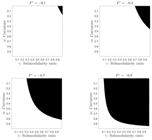
For the sake of visualization, we let f(∅) = −1, f(V) = 1, f(S∗) = F∗ ∈ [−1,1]. Figure 1 shades the area where the guarantee for the forward greedy algorithm is better than the one for the reverse greedy algorithm. By decreasing the value of F∗ from 0 to −1, one can observe that the area where the forward greedy guarantee is better, expands. When F∗ is small, and the function is close to being both submodular and supermodular, the forward greedy guarantee is more desirable. In fact, [7, Propositions 4 and 5] prove that there is no performance guarantee for the forward greedy algorithm unless both the submodularity ratio and the curvature are utilized, simultaneously. When F∗ is large enough, F∗ ≥ 0, the effect of f(∅) on the forward greedy guarantee is more dominant, thus, the reverse greedy outperforms the forward greedy for all (α, γ) pairs. Note that for other values off(∅) or f(V), the observations can differ. In practice, it could be useful to implement both greedy algorithms (which can be done efficiently with polynomial time complexity) and choose the best out of the two.
Our future work will be focused on obtaining the problem instances for which these guarantees are potentially tight.
5. Acknowledgments
The authors would like to thank Professor Victor Il’ev for his helpful feedback on existing bounds on the worst-case behaviour of greedy algorithms, Dr. Yatao An Bian for early discussions on the literature for existing properties of set functions.
Figure 1: For eachF∗value, the shaded regions represent the (α, γ) pairs for which the forward greedy algorithm outperforms the reverse greedy algorithm. ForF∗≥0, the reverse greedy algorithm outperforms the forward greedy algorithm for any (α, γ) pair.
References
[1] A. A. Bian, J. M. Buhmann, A. Krause, and S. Tschiatschek, “Guarantees for greedy maximization of non- submodular functions with applications,” in34th ICML, 2017, pp. 498–507.
[2] L. Chen, M. Feldman, and A. Karbasi, “Weakly submodular maximization beyond cardinality constraints: Does randomization help greedy?” in35th ICML, 2018, pp. 804–813.
[3] E. R. Elenberg, R. Khanna, A. G. Dimakis, S. Negahban et al., “Restricted strong convexity implies weak submodularity,”Annals of Statistics, vol. 46, no. 6B, pp. 3539–3568, 2018.
[4] A. Clark, B. Alomair, L. Bushnell, and R. Poovendran, “Submodularity in input node selection for networked linear systems: Efficient algorithms for performance and controllability,”IEEE Contr. Syst. Magazine, vol. 37, no. 6, pp. 52–74, 2017.
[5] A. Clark, L. Bushnell, and R. Poovendran, “On leader selection for performance and controllability in multi- agent systems,” in51st CDC, 2012, pp. 86–93.
[6] B. Guo, O. Karaca, T. Summers, and M. Kamgarpour, “Actuator placement for optimizing network performance under controllability constraints,” in58th CDC, 2019.
[7] ——, “Actuator placement under structural controllability using forward and reverse greedy algorithms,”IEEE Trans. on Aut. Contr., 2021.
[8] V. Tzoumas, M. A. Rahimian, G. J. Pappas, and A. Jadbabaie, “Minimal actuator placement with bounds on control effort,”IEEE Trans. on Contr. of Netw. Syst., vol. 3, no. 1, pp. 67–78, March 2016.
[9] B. P. Gerkey and M. J. Matari´c, “A formal analysis and taxonomy of task allocation in multi-robot systems,”
The Int. J. of Rob. Res., vol. 23, no. 9, pp. 939–954, 2004.
[10] S. Jorgensen, R. H. Chen, M. B. Milam, and M. Pavone, “The matroid team surviving orienteers problem:
Constrained routing of heterogeneous teams with risky traversal,” inIROS. IEEE, 2017, pp. 5622–5629.
[11] L. Zhou, V. Tzoumas, G. J. Pappas, and P. Tokekar, “Resilient active target tracking with multiple robots,”
IEEE Rob. and Aut. Letters, vol. 4, no. 1, pp. 129–136, 2018.
[12] D. Tihanyi, “Multi-robot extension for safe planning under dynamic uncertainty,”Master thesis, ETH Z¨urich, 2021. [Online]. Available: https://www.research-collection.ethz.ch/handle/20.500.11850/471229
[13] D. Tihanyi, Y. Lu, O. Karaca, and M. Kamgarpour, “Multi-robot task allocation for safe planning under dynamic uncertainty,”arXiv submission, 2021.
[14] H.-S. Shin and P. Segui-Gasco, “Uav swarms: Decision-making paradigms,”Encyclopedia of aerospace engineer- ing, pp. 1–13, 2010.
[15] L. A. Wolsey and G. L. Nemhauser,Integer and combinatorial optimization. John Wiley & Sons, 1988, vol. 55.
[16] G. L. Nemhauser, L. A. Wolsey, and M. L. Fisher, “An analysis of approximations for maximizing submodular set functions—i,”Math. Prog., vol. 14, no. 1, pp. 265–294, 1978.
[17] M. L. Fisher, G. L. Nemhauser, and L. A. Wolsey, “An analysis of approximations for maximizing submodular set functions—ii,” inPolyhedral Combinatorics. Springer, 1978, pp. 73–87.
[18] M. Conforti and G. Cornu´ejols, “Submodular set functions, matroids and the greedy algorithm: tight worst-case bounds and some generalizations of the rado-edmonds theorem,”Discrete App. Math., vol. 7, no. 3, pp. 251–274, 1984.
[19] M. Sviridenko, J. Vondr´ak, and J. Ward, “Optimal approximation for submodular and supermodular optimiza- tion with bounded curvature,”Math. of Oper. Res., vol. 42, no. 4, pp. 1197–1218, 2017.
[20] T. Zhang, “Adaptive forward-backward greedy algorithm for learning sparse representations,”IEEE Trans. on Inf. Theory, vol. 57, no. 7, pp. 4689–4708, 2011.
[21] J. A. Tropp, “Greed is good: Algorithmic results for sparse approximation,” IEEE Trans. on Inf. Theory, vol. 50, no. 10, pp. 2231–2242, 2004.
[22] M. Chrobak, C. Kenyon, and N. Young, “The reverse greedy algorithm for the metric k-median problem,”Inf.
Processing Letters, vol. 97, no. 2, pp. 68–72, 2006.
[23] V. Il’ev and S. Il’eva, “On minimizing supermodular functions on hereditary systems,” inOptimization Problems and Their Applications, 2018, pp. 3–15.
[24] V. Il’ev, “Hereditary systems and greedy-type algorithms,”Discrete App. Math., vol. 132, no. 1-3, pp. 137–148, 2003.
[25] A. Schrijver, Combinatorial Optimization: Polyhedra and Efficiency, ser. Algorithms and Combinatorics.
Springer, 2003, no. 1. k. [Online]. Available: https://books.google.ch/books?id=mqGeSQ6dJycC
[26] J. Oxley,Matroid Theory, ser. Oxford graduate texts in mathematics. Oxford University Press, 2006. [Online].
Available: https://books.google.ch/books?id=puKta1Hdz-8C
[27] D. Welsh, Matroid Theory, ser. Dover books on mathematics. Dover Publications, 2010. [Online]. Available:
https://books.google.ch/books?id=QL2iYMBLpFwC
[28] A. Krause and C. E. Guestrin, “Near-optimal nonmyopic value of information in graphical models,” inConf.
on Uncertainty in AI, 2005.
[29] F. Bach, “Learning with submodular functions: A convex optimization perspective,”Found. and Tr. in Mach.
Lrn., vol. 6, no. 2-3, pp. 145–373, 2013.
[30] B. Lehmann, D. Lehmann, and N. Nisan, “Combinatorial auctions with decreasing marginal utilities,”Games and Economic Behavior, vol. 55, pp. 270–296, 01 2001.
[31] A. Das and D. Kempe, “Submodular meets spectral: Greedy algorithms for subset selection, sparse approxima- tion and dictionary selection,” in28th ICML, 2011, pp. 1057–1064.
[32] O. Karaca and M. Kamgarpour, “Exploiting weak supermodularity for coalition-proof mechanisms,” in57th CDC. IEEE, 2018, pp. 1118–1123.
[33] A. Krause and D. Golovin, “Submodular function maximization,”Tractability, vol. 3, pp. 71–104, 01 2011.
[34] V. Tzoumas, A. Jadbabaie, and G. J. Pappas, “Resilient non-submodular maximization over matroid con- straints,”arXiv preprint arXiv:1804.01013, 2018.
[35] J. Edmonds, “Matroids and the greedy algorithm,”Math. Prog., vol. 1, no. 1, pp. 127–136, 1971.
[36] D. Welsh, “On matroid theorems of edmonds and rado,”Journal of the London Mathematical Society, vol. 2, pp. 251–256, 1970.
[37] T. Summers and M. Kamgarpour, “Performance guarantees for greedy maximization of non-submodular con- trollability metrics,” in18th ECC, 2019, pp. 2796–2801.
[38] V. Il’ev and N. Linker, “Performance guarantees of a greedy algorithm for minimizing a supermodular set function on comatroid,”EJOR, vol. 171, no. 2, pp. 648–660, 2006.
[39] O. Karaca, B. Guo, and M. Kamgarpour, “A comment on performance guarantees of a greedy algorithm for minimizing a supermodular set function on comatroid,”EJOR, vol. 290, no. 1, pp. 401–403, 2020.