Research Collection
Master Thesis
Multi-robot extension for safe planning under dynamic uncertainty
Author(s):
Tihanyi, Dániel Publication Date:
2021-01-11 Permanent Link:
https://doi.org/10.3929/ethz-b-000471229
Rights / License:
In Copyright - Non-Commercial Use Permitted
This page was generated automatically upon download from the ETH Zurich Research Collection. For more information please consult the Terms of use.
The text font of “Automatic Control Laboratory” is DIN Medium C = 100, M = 83, Y = 35, K = 22
C = 0, M = 0, Y = 0, K = 60
Logo on dark background K = 100 K = 60 pantone 294 C
pantone Cool Grey 9 C
Automatic Control Laboratory
Master Thesis
Multi-robot extension for safe planning under dynamic uncertainty
Tihanyi D´aniel January 11, 2021
Advisors
Prof. Maryam Kamgarpour, Dr. Or¸cun Karaca, Yimeng Lu
Contents
1 Introduction 4
2 Notations 6
3 Preliminaries 7
4 Two-stage multi-robot safe planning framework 10
4.1 Single-robot safe planning problem . . . 10
4.1.1 Map model . . . 11
4.1.2 Robot dynamics . . . 12
4.1.3 Hazard dynamics . . . 12
4.1.4 Target execution . . . 12
4.1.5 Combined state space . . . 13
4.1.6 Controller synthesis via dynamic programming . . . 14
4.2 Multi-robot task allocation problem . . . 15
4.3 Full-fleet safe planning framework . . . 16
5 Greedy approach for multi-robot task allocation under dynamic uncertainties 18 5.1 Forward greedy algorithm . . . 18
5.1.1 Algorithm formulation . . . 18
5.1.2 Performance guarantee . . . 20
5.1.3 Distributed algorithm formulation . . . 20
5.2 Reverse greedy algorithm . . . 22
5.2.1 Algorithm formulation . . . 22
5.2.2 Performance guarantee . . . 24
5.2.3 Distributed algorithm formulation . . . 24
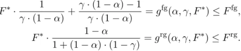
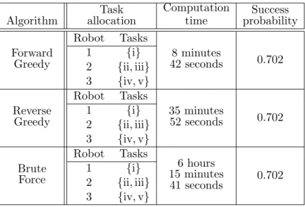
5.3 Comparison of performance guarantees for forward and reverse greedy approaches 26 6 Numerical case studies 29 6.1 Performance comparison of task allocation algorithms . . . 29
6.2 Counterexample for the usage of the multiplicative group success . . . 32
6.3 Performance comparison of full-fleet safe planning and two-stage multi-robot safe planning . . . 35
7 Conclusions 38 8 Appendix 42 8.1 Calculating the contamination risk pkH . . . 42
8.2 Definition of the combined transition kernelτSk . . . 43
8.3 Proof of Equation (13) . . . 45
8.4 Full-fleet safe planning problem . . . 47
8.5 Mild conditions for multiplicative group success to be a lower bound on the prob- ability of group success . . . 49
8.6 Performance guarantee for the forward greedy algorithm . . . 50
8.7 Performance guarantee for the reverse greedy algorithm . . . 52
8.8 Example hazard modelτY . . . 54
Abstract
Safe planning problem arises in many applications including autonomous driving and explo- ration scenarios. In this thesis, we focus on a particular case studied for emergency rescue missions. The main challenge of such problems is the computational complexity of handling a dynamic uncertainty, e.g., a spreading hazard. A multi-agent extension can potentially im- prove the safety of the mission. However, it further increases the computational complexity with the need to consider exponentially many possible task-robot combinations. To over- come these computational issues, we propose a two-stage framework splitting the multi-robot safe planning problem into a low-level single-agent safe planning problem and a high-level multi-robot task allocation problem. For single-agent safe planning, we utilize an efficient Monte-Carlo sampling-based approximation to handle the dynamic uncertainty. For the task allocation problem, we use forward and reverse greedy heuristics to obtain approximate so- lutions. These algorithms are equipped with provable performance bounds on the safety of the resulting approximate solutions. Finally, we present several case studies on example environments to compare the performance of these different algorithms.
1 Introduction
The usage of multi-agent systems is of increasing interest in robotics [1]. In many appli- cations, a fleet of robots has to operate cooperatively to reach a common goal, such as in robotic- teamwork football games [2], automated guided vehicle systems in warehouses [3], surveillance or monitoring missions [4–6] and others. Systems using multiple agents enjoy trivial advan- tages over single-agent solutions. They can distribute tasks or workload among themselves and reduce execution time by working in parallel. This makes multi-agent solutions capable of han- dling problems with higher complexity, larger number of tasks, carrying out more deliveries at a given time span, or covering larger areas in surveillance missions than their single-agent counterparts. Multi-agent systems are also highly reliable and robust against failure, since the system can still continue working even in case of multiple agents failing. These advantages, however, come with an increased computational complexity which requires the usage of more sophisticated approaches and algorithms. The challenges and the tools can vary depending on the application. This thesis aims to extend the existing research in planning for safety-critical rescue missions to a multi-agent framework. This requires a combined study of two fields: safe planning and multi-agent task allocation.
The goal of safe planning is to maximize the probability of successfully executing a given set of tasks by deriving control policies in a potentially hostile environment. The applications include safe autonomous driving [7], exploration scenarios [8], or as in our case, emergency rescue missions with dangerously spreading fire or toxic contamination threatening the life of survivors [9]. This problem comes with several challenges to provide solutions in such applications. A major challenge originates from modelling the dynamic uncertainties of the environment caused by the evolving hazard. Many approaches either use restrictive Gaussian models [10,11] or more general yet computationally intractable Markov models [12]. We build on the previous work of [13] which provides a trade-off between both issues by using a Monte-Carlo sampling-based approximation to reduce the state space required for its Markov model. Another challenge originates from high-level decision making such as the one of ordering sequential execution of multiple tasks. To handle both these high-level decisions and the low-level point-to-point path planning, an extended state space definition is used in [9, 13] incorporating the execution of tasks into the problem definition. The optimal policies are derived using the well-known dynamic programming algorithm [14].
Multi-agent task allocation problems aim to decide which tasks should be executed by which agents in order to maximize a collective success measure. In their general form, such set partition problems are known to be NP-hard, hence the usage of heuristics as an approximate solution method is an attractive option for their scalability [15]. Variants of the greedy algo- rithm are widely-used in combinatorial optimization literature [4, 5, 16–24]. A valid allocation constituting a partition is known to be given by the base of a matroid where the ground set is all agent-task pairs. Our goal is then to maximize the set function mapping allocations to some collective objective. The greedy algorithm achieves this by iteratively adding the best
agent-task pair towards a valid allocation. Under a submodular objective function greedy en- joys 1/2 performance guarantee [4, 16–19, 21]. The probability of successful navigation in the emergency rescue missions is, however, non-submodular. To mitigate this issue, the concepts of submodularity ratio and curvature were introduced, which measure how far a function is from being submodular and supermodular, respectively. Previous works on non-submodular set function maximization used the notion of the submodularity ratio [22, 25], the curvature [24, 26]
or both [20, 23] to provide performance guarantees for the greedy algorithm. We build on these studies and provided two novel performance guarantees for greedy algorithms in matroid opti- mization. The first is on the forward greedy algorithm, improving and generalizing [16] and [22]
by the inclusion of both the submodularity ratio and curvature properties, respectively. The second is on the reverse greedy algorithm improving and generalizing [27] by removing the strong requirement of using the notion of total curvature, and [23] by reducing the requirement on the cardinality of the ground set.
It is important to note alternative approaches to solve set partition problems, coinciding with a multi-agent task allocation problem. The authors in [28] consider a set partitioning problem, where each subset of tasks is associated with a fixed cost for agents, and the goal is to find the optimal partitioning. This approach requires the cost of each subset to be evaluated in advance. In our case, this can only be obtained by solving the single-agent safe planning problem for all these subsets, which would be computationally demanding. Another approach would be to use a bipartite graph listing all agents and tasks as vertices where the edges, each associated with a cost, represent the assignment between them, see [29]. In our multi-agent safe planning problem, we cannot define such costs for each task-agent pair independently, since our objective is non-additive (in other words, non-modular). We can only define such costs for subsets of tasks allocated to an agent. In conclusion, none of the aforementioned approaches are applicable for our purposes.
Combining safe planning and multi-agent task allocation, our contribution is to provide a scalable framework for the multi-robot emergency rescue scenario. The usage of multiple agents could potentially improve success probability, the system would be able to handle more tasks, hence more survivors could be saved with higher probability. On the high-level, task allocation aims to allocate each survivor to a robot. According to the taxonomy in [15], this problem would be classified as a multi-task robot, single-robot task, instantaneous assignment1 problem (MT-SR-IA). On the other hand, notice that each robot can handle multiple tasks. Task allocation is solved via greedy algorithms. We analyze two different algorithms, the forward and reverse greedy approaches, and compare them both in terms of their theoretical performances, experimental performances, and computational times. In doing that, we provide two novel performance guarantees for these greedy algorithms applied to general matroid optimization problems. On the low-level, we derive control policies for each agent for a given subset of tasks, while maximizing the probability of successful navigation. This low-level framework is an efficient implementation of the ones in [9, 13], where a Monte-Carlo sampling based algorithm is
1Since we allocate the tasks to the robots before execution, we have the so-called instantaneous assignment setting.
proposed to overcome the computational burdens of Markovian models of stochastically evolving hazard.
We organize this thesis report as follows. Preliminaries summarize the necessary math- ematical background for this report in Section 3. In Section 4, we introduce the two-stage framework by formulating both the single-robot safe planning and the multi-robot task alloca- tion problems. Next, we propose the two greedy approaches in Section 5, the forward and reverse greedy algorithms. Finally, we show three case studies comparing algorithm performance, see Section 6, and we then conclude the paper in Section 7.
2 Notations
Unless stated otherwise, we use the following conventions when naming variables through- out the thesis report. We denote finite sets by block letters, their elements by lower case letters, and families of sets by calligraphic block letters. Let X be a finite set. We use the definition of indicator function 1¯x :X → {0,1} for an element ¯x ∈ X and 1X¯ :X → {0,1} for a subset X¯ ⊂X. They are defined the following way
1x¯(x) =
1 if x= ¯x, 0 otherwise,
1X¯(x) =
1 if x∈X,¯ 0 otherwise.
Furthermore, let|X|denote the size of a finite setX. We use the notation∧for the logical ‘AND’
and ∨ for the logical ‘OR’ in mathematical statements. Letp(x= ¯x) denote the probability of a discrete random variablex taking the value of ¯x.
3 Preliminaries
In this section, we introduce well-studied notions from discrete mathematics literature [30–
33]. These notions will be used for the derivations in the remainder of this report. Let W be a nonempty ground set andf : 2W →Ra set function for the following definitions.
Definition 1 (Monotonicity properties) The set function f is non-decreasing if for all A ⊆ B ⊆W, f(A) ≤f(B). We call −f non-increasing. If the inequality is strict, then f is strictly increasing and −f is strictly decreasing.
Definition 2 (Discrete derivative) For the set function f, A ⊆ W and e ∈ W, the discrete derivative of f at A with respect toe is given by
ρf(e|A) :=f(A∪ {e})−f(A).
We simply use the notationρ(e|A), if the functionf is clear from the context. Moreover for any set B⊂W, we will generalize the definition above to denote ρ(B|A) =f(A∪B)−f(A).
Definition 3 (Submodularity) A non-decreasing set function f is submodular if it holds that
ρ(e|B)≤ρ(e|A), (1)
for all A⊆B⊆W, for all e∈W \B.
Submodularity is a useful property commonly used in combinatorics. Equation (1) ex- presses that the marginal gains of f are decreasing when expanding the set A to B, which happens to be the case in many realistic examples, see [33–35]. Many set function optimiz- ing algorithms take advantage of this notion, such as the greedy algorithm used later in this report. Unfortunately, the objective functions used in many problems, including ours, do not have the submodular property. Instead, these problems allow the use of submodularity ratio describing how far a non-submodular set function is from being submodular. This property was first introduced in [25].
Definition 4 (Submodularity ratio) The submodularity ratio of a nondecreasing set function f is the largest scalarγ ∈R+ such that
γ·ρ(e|B)≤ρ(e|A), (2)
for all A⊆B⊆W, for all e∈W \B.
It can easily be verified that f is submodular if and only if γ = 1, and we also have γ ∈ [0,1]. For derivations, kindly refer to [20]. Furthermore, there exist an alternative but
non-equivalent submodularity ratio notion [20, 36]: thecumulative submodularity ratio of a non- decreasing set function f is the largest scalarγ0 ∈R+ such that
γ0·ρ(B|A)≤ X
e∈B\A
ρ(e|A), (3)
for all A, B ⊆ W. The submodularity ratio of Equation (2) satisfies the inequalities listed in Equation (3), but the reverse argument does not necessarily hold. Hence, γ ≤ γ0 [23, Ap- pendix B]. Later in Sections 5.1 and 5.2, we discuss the necessity of utilizing this notion as per Definition 4 for the guarantee we derive for the greedy algorithms.
Definition 5 (Supermodularity) A non-decreasing set function f is supermodular if it holds that
ρ(e|A)≤ρ(e|B), (4)
for all A⊆B⊆W, for all e∈W \B.
Supermodularity is the property describing that the marginal gain of f is increasing when expanding the setAtoB. Similar to the discussions provided for the submodularity ratio, whenever supermodularity is not found, it may instead be possible to use the notion ofcurvature to describe how far a non-supermodular function is from being supermodular.
Definition 6 (Curvature) The curvature of a non-decreasing set function f is the smallest scalar α∈R+ such that
(1−α)·ρ(e|A)≤ρ(e|B), (5)
for all A⊆B⊆W, for all e∈W \B.
It can easily be verified that f is supermodular if and only if α = 0, and we also have α ∈ [0,1]. For derivations, kindly refer to [20]. Finally, note that it is also possible to have cumulative definitions of the curvature, similar to that of Equation (3). However, for our deriva- tions in Sections 5.1 and 5.2, we draw special attention on where we require the inequalities in Equation (5).
Complex constraints in many combinatorial optimization problems can be modelled by using notions from matroid theory introduced in the following. Reformulating this way gener- alizes the constraints and helps to provide performance guarantees.
Definition 7 (Matroid). A matroid is a pair M= (W,I), such that I ⊆2W is a collection of subsets ofW called the independent set satisfying the two following properties
(i) A⊆B ⊆W and B ∈ I implies A∈ I
(ii) A, B ∈ I and |B|>|A|implies ∃e∈B\A such thatA∪ {e} ∈ I.
The concept of a matroid is considered to be a generalization of linear-independence well known from linear algebra. We introduce a special type of matroid used for the problem formulations of this report, the partition matroid.
Definition 8 (Partition matroid) The pair M = (W,I) is a partition matroid if a partition of W exists characterized by {Bi}i=1,...,n, where W =
n
S
i=1
Bi and Bi ∩Bi0 = ∅ for all pairs i, i0 ∈ {1, . . . , n}, furthermore there exist a set of positive integers li ∈Z+ for all i = 1, . . . , n, such that
I ={A⊆W | |A∩Bi| ≤li,∀i= 1, . . . , n}.
Furthermore, we also use the following matroid theory related properties.
Definition 9 (Base of a matroid) Let M = (W,I) be a matroid. We call B ∈ I a base of matroid M, if |A| ≤ |B|for allA∈ I. In other words, a base of a matroid is an inclusion-wise maximal independent set. Notice, that every base has the same cardinality.
Definition 10 (Dual of a matroid) For a matroid, M= (W,I), the dual matroid M¯ = (W,I)¯ is defined so defined so that the bases B¯ ∈ I¯ are exactly the complements of the bases B ∈ I, that is, B¯ =W \B.
4 Two-stage multi-robot safe planning framework
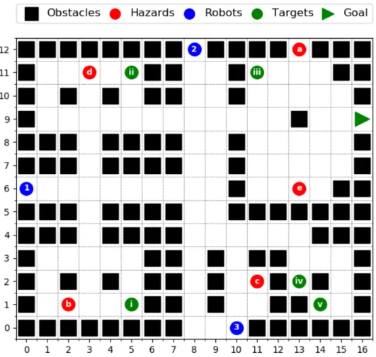
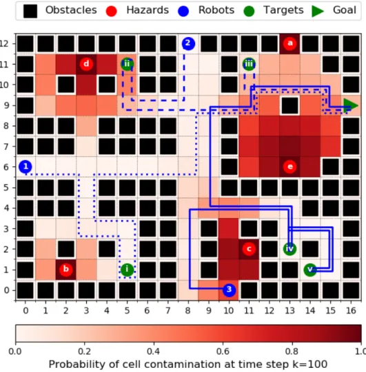
In this section, we introduce themulti-robot safe planning problem and propose a frame- work that provides a computationally tractable solution. Consider a fleet of autonomous agents navigating through an environment with a stochastically evolving hazard, for example, a fire inside a building. The mission of the fleet is to visit a set of known targets and then get out safely (e.g. rescuing survivors). Each target is required to be visited once by any robot. The map of the environment, the initial position of the robots, the areas initial contaminated by the hazard, and the stochastic model of the dynamics of both the hazard and the robots are assumed to be known. The multi-robot safe planning problem aims to designcontrol policies for the robots. These control policies maximize theprobability of success – the probability of suc- cessfully finishing the mission. However, planning for multiple robots is computationally much more challenging than planning for a single robot. Hence our framework splits the problem into the following two hierarchical stages: high-level task allocation (dividing the targets between robots) and low-level path planning (optimizing control policies for each robot individually for a subset of assigned targets). We call this thetwo-stage multi-robot safe planning framework. The low-level stage introduced in Section 4.1 aims to obtain an optimal control policy for a single robot maximizing the probability of successfully visiting only a chosen subset of all targets. The high-level stage, which builds upon the low-level one, is a multi-robot task allocation problem aiming to divide the targets among robots and is described in Section 4.2. To justify the need for splitting the problem into stages as in our framework, we formulate a safe planning problem for the whole fleet combined in Section 4.3 and show its computational burdens. Throughout this section, we use an example multi-agent planning problem to illustrate our framework, see Figure 2.
4.1 Single-robot safe planning problem
This section introduces the low-level singler-robot safe planning framework for a single agent aiming to obtain an optimal control policy by maximizing the probability of successfully visiting a set of targets and leave the environment while avoiding the evolving hazard. The problem formulation is based on previous works in path planning under dynamic uncertainties, namely, [9] and [13], and presented as follows. We first concisely introduce this model and leave the details in the following subsections. We start by considering a single-robot system, describe the environment with a discretized map, then introduce the robot and hazard evolution dynam- ics. Next, we show how the agent keeps track of the high-level target execution. We then define a combined state space for path planning considering the robot dynamics, the target execution and hazard avoiding aspects. Finally, we define the controller synthesis problem and present a dynamic programming algorithm that solves this problem. To obtain a tractable version of this approach, we propose an approximation based on Monte-Carlo sampling to overcome the computational issues caused by the presence of dynamic uncertainties.
Figure 2: Example environment. The fleet of robots have to reach the goal position after cooperatively visiting the targets while avoiding the stochastically evolving hazards.
4.1.1 Map model
We define a discretized model of the map where the robot operates. Let Mm×n={(a, b)|a∈ {0, . . . , m−1}, b∈ {0, . . . , n−1}},
be an m×n-sized grid-shaped map (the grid length equals to 1) and O ⊂ Mm×n be a set of obstacles (e.g., walls) untraversable for the robot. Then, X = Mm×n\O is the set of all traversable positions. Furthermore, for all x∈X let
N(x) =
x0∈X| kx0−xk2 = 1 , D(x) =n
x0 ∈X| kx0−xk2 =√ 2o
,
be the neighboring and diagonally neighboring positions forx, respectively. We use the notation kx0 −xk2 for the Euclidean distance between points x and x0. The usage of a discredited map simplifies the formulation from a non-convex continuous optimization problem to an easier combinatorial optimization problem. It is a reasonable approximation of the environment also used in [9] and [13].
4.1.2 Robot dynamics
We introduce the dynamics of the motion of the robot. We define a set of possible inputs:
U ={Stay,North,East,South,West}. Each inputu∈U is associated with a direction dStay= (0,0), dNorth= (0,1), dEast= (1,0), dSouth= (0,−1), dWest= (−1,0).
In each position x∈X, the set of
U(x) ={u∈U|x+du ∈X} ⊆U, are the inputs available to the robot.
The motion of robot r is defined by a stochastic Markov process xk+1 ∼ τX · |xk, uk , k∈ {0,1, . . .}with initial positionx0r ∈X, whereτX :X×X×U →[0,1] denotes the transition kernel between xk ∈ X at time step k and xk+1 ∈ N(x) at step k+ 1 under control input uk ∈ U(xk). Note that different robots can be equipped with different dynamics. We say that the robot dynamics are deterministic, if for all xk∈X and uk∈U(xk)
τX
xk+1|xk, uk
=1xk+duk(xk+1). (6)
4.1.3 Hazard dynamics
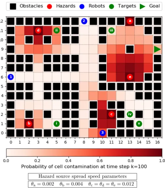
We introduce the model of the hazard and how it spreads across the map. Let Y = 2X be the hazard state space. Each element y ∈ Y denotes a set of contaminated cells being a subset of the reachable mapX. The stochastic Markov processyk+1 ∼τY · |yk
,k∈ {0,1, . . .} defines the hazard evolution dynamics with transition kernelτY :Y ×Y →[0,1] between states yk∈Y at time stepkandyk+1∈Y at stepk+ 1. At time 0, we assume the hazard statey0 ∈Y to be known to the robot.
4.1.4 Target execution
During the execution of the mission, the agent needs to keep track of which target loca- tions have already been visited. To this end, we introduce the followingtarget execution state.
First we defineTr⊂X as thetarget list of robot r, the set of all target locations the agent has to visit. Then we define the set Q= 2Tr and the target execution state qk ⊆ Tr at time step k, where qk ∈Q for all k. The transition at time step k from qk toqk+1 given the robot is at positionxk+1 at step k+ 1 is described by the following time homogeneous transition kernel
τQ(qk+1|qk, xk+1) =
1 if qk+1=qk∪(xk+1∩Tr), 0 otherwise,
whereτQ :Q×Q×X →[0,1]. Every time one of the target positionsxk+1 ∈Tr is visited, it is added to the listqk+1. For any other non-target positionxk+1 ∈/ Tr, we have xk+1∩Tr=∅and qk+1 = qk stays the same. If a target position xk+1 ∈Tr is visited more then one time, hence xk+1 ∈qk, thenqk+1=qk∪ {xk+1}=qk.
4.1.5 Combined state space
In this section, we define the combined state space of the agent in order to model the complex mission of motion, target collection and hazard avoidance. At time step k the state should contain both the robot location xk ∈ X and the target execution state qk ∈ Q. Some pairs of (qk, xk) are impossible to occur specifically, when xk ∈Tr but xk ∈/ qk, hence we can reduce the size of the state space by removing these pairs. We further assume that the agent cannot observe the state of the hazardyk∈Y, which is a reasonable assumption in most realistic scenarios, hence we do not includeykin the state space2. However, acontamination state noted by sH should be introduced to capture the contamination of the robot. The agent transmits into state sH if it moves to a contaminated area xk∈yk, after which it cannot leave this state anymore. Reaching the contamination state indicates an unsuccessful mission. We can now write the combined state space as follows
S={sH} ∪(Q×X)\ {(q, x)|x∈Tr∧x /∈q}. (7) We can further specify the goal location asxG∈Xand thegoal state denoted bysG= (Tr, xG).
The state sG indicates a successful mission, where every target is visited and the robot has reached the safe goal location without getting contaminated. We also define the initial state for robot r ass0r = (∅, x0r), where no targets are visited and the robot is at the initial position x0r. The state s0r is certain and known to the agent, since x0r, the initial position of robot r is assumed to be given.
Although the agent cannot observe the state of the hazardyk∈Y at a certain time step k, it can still use the knowledge of the hazard dynamics τY and the initial hazard state y0. To this end, we define the function pkH :X×X →[0,1] describes the contamination risk, the risk the robot takes while moving to a new grid cell at a given time stepk. The value ofpkH(xk+1, xk) for the pairxk+1 andxkis equal to the probability ofxk+1 ∈yk+1 getting contaminated at time step k+ 1, given that xk ∈/ yk is not contaminated at step k. For values xk+1 = ¯xk+1 and xk = ¯xk
pkH(¯xk+1,x¯k) =P(xk+1∈yk+1|xk∈/yk, xk+1 = ¯xk+1, xk= ¯xk). (8) We provide the details of calculatingpkH in Appendix 8.1. Due to the exponentially increasing size of|Y|= 2|X|, the precise calculation of functionpkH described in Appendix 8.1 is computationally intractable. In order to overcome this issue, a Monte-Carlo sampling based algorithm is proposed
2For further justification whyykshould not be included in the state space, let us study the complexity ofX,Q andY. The size ofX depends on the size of the map, whereas the number of target execution states|Q|= 2|Tr| grows exponentially with the size ofTr. In practice, we have|X| |Tr|. Thus, the size of the hazard state space
|Y|= 2|X| is the main source of complexity. IncludingY in the state space would make the problem intractable even for small maps.
in [13, Algorithm 1], which provides a tractable approximation ofpkH. For the rest of the report we refer to pkH as the approximate value obtained by [13, Algorithm 1].
The evolution of the combined state of the agent can now be described by the following stochastic process defined by transition kernel τSk:S×S×U →[0,1]. Given that the robot is in state sk at time stepk, the probability of getting into statesk+1 at step k+ 1 by applying control input uk can be written as follows (see Appendix 8.2)
τSk(sk+1|sk, uk) =
1 if sk+1 =sk∈ {sG, sH}, P
xk+1∈X
pkH(xk+1, xk)
×τX(xk+1|xk, uk) if sk+1 =sH
∧ sk= (qk, xk)∈ {s/ G, sH}, 1−pkH(xk+1, xk)
×τQ(qk+1|qk, xk+1)
×τX(xk+1|xk, uk) if sk+1 = (qk+1, xk+1)6=sH
∧ sk= (qk, xk)∈ {s/ G, sH},
0 otherwise.
(9)
Both the goal sG and hazardsH states are defined to beabsorbing, which means, once they are reached, the system state does not change anymore. In any other statessk= (qk, xk)∈ {s/ G, sH}, the agent can either get contaminated and reach state sH or move to another state following the dynamics defined by transition kernelsτX and τQ.
4.1.6 Controller synthesis via dynamic programming
Based on the previously described combined state space and transition dynamics, we state the success probability maximizing optimization problem. We also propose a dynamic programming algorithm to solve this problem and obtain the optimal control policy. We assume that robot r, a set of target locations Tr ⊂ X, the initial state s0r and a finite time horizon N ∈ N>0 is given. We aim to compute the optimal (that is success probability maximizing) closed-loop control policy πr(Tr) ={µ0r, . . . , µNr −1}as a function ofTr, whereµkr :S→U refers to the control law at time step k, so that uk = µkr(sk). We denote the optimal probability of success under the optimal control policy πr(Tr) by fr(Tr). Furthermore, the probability of success fr(π, Tr) under a generic control policy π = {µ0, . . . , µN−1} can be described by reaching the goal state sk=sG at any step within the given time horizonk≤N while avoiding the contamination state sk =sH at all time steps k ={0, . . . , N}. Since both sH and sG are absorbing, the conditionsN =sG is sufficient for a successful mission as shown below
fr(π, Tr) =P sN =sG|π
. (10)
Our goal is then to solve
πr(Tr) = arg max
π
fr(π, Tr). (11)
Problem (11) can be solved using the well known dynamic programming algorithm [14]: For k=N, let us define VN(sN) =1sG(sN) as thevalue function, while for 1≤k≤N,
Vk−1(sk−1) = max
u∈U(xk−1)
( X
sk∈S
τSk−1(sk|sk−1, u)·Vk(sk) )
. (12)
Now µkr(sk) can be obtained as the optimal u ∈ U(xk) at step k. Furthermore it holds (see Appendix 8.3), that
fr(Tr) =fr(πr, Tr) = max
π fr(π, Tr) =V0(s0r). (13) 4.2 Multi-robot task allocation problem
In this section, we formulate the high-level task allocation problem aiming to optimally assign the targets among the agents. Let T be the set of all targets andR the set of all robots.
A valid task allocation assigns each task to exactly one agent by dividing set T into partitions {Tr}r∈R, where Tr ⊂ T for all r ∈ R, Tr∩Tr0 = ∅ for any pair r, r0 ∈ R where r 6= r0 and S
r∈RTr = T. Each partition Tr represents the subset of targets assigned to robot r. We aim to find the optimal task allocation which maximizes the probability of successfully finishing the mission of visiting every target without getting any of the agents contaminated 3. We use the multiplicative group success as the objective function defined by
F({Tr}r∈R) = Y
r∈R
fr(Tr), (14)
where the values of fr(Tr) are obtained by solving the single-robot path planning problem introduced in Section 4.1 for each r ∈ R (see Equation (13)). Note that the multiplicative group success equals the product of single-agent success probabilities. Hence it assumes these success probabilities to be independent of each other. This assumption does not hold in general.
However, in most cases, one of the robots succeeding makes it more probable for the others to succeed as well (see Appendix 8.5). Under this mild condition, the multiplicative group success can serve as a good and computationally tractable approximation. Now we can formulate the task allocation problem as follows
F∗= max
{Tr}r∈R
Y
r∈R
fr(Tr) s.t. Tr∩Tr0 =∅,∀r6=r0, [
r∈R
Tr =T. (15)
Every task is allocated to exactly one robot. Following this argument, each task can
3According to the taxonomy in [15], this problem can be classified as an NP-hard multi-task robot, single- robot task, instantaneous assignment task allocation problem (MT-SR-IA). Multi-task robot – because one robot can visit multiple targets, single-robot task – since it is enough for targets to be visited by only a single robot, and instantaneous assignment – since tasks are allocated only once before the run and not continuously during execution.
be allocated to any robot among |R| different robots. Hence there are |R||T| possible alloca- tions in total. Therefore, the problem is exponential in the number of tasks, which motivates using polynomial-time heuristic algorithms to obtain approximate solutions. We propose such algorithms in Section 5 and provide detailed descriptions.
Furthermore, adding a task to the target list of a robot cannot increase its success prob- ability. Because when one additional task is added to the task list of a robot, the updated path due to this additional task either becomes longer or deviate from the original path in most of the cases. Both of them decreases the probability of success. To capture this, we assume the individual functionsfr to be strictly and bounded decreasing, hence∃f
r, fr∈R such that 0< f
r ≤fr(Tr)−fr(Tr∪t)≤fr <1, (16) for all Tr (T, for all t∈ T \Tr and every r ∈R. We use this assumption in Section 5. This assumption might occasionally be violated if task t already lies on the path of robot r when executing task list Tr. In this rare case fr(Tr∪t) =fr(Tr).
4.3 Full-fleet safe planning framework
We generalize the single-robot planning formulation introduced in Section 4.1 and propose thefull-fleet safe planning frameworkfor|R| ≥1 as an alternative approach for solving the multi- robot safe planning problem. We also show the computational burdens of this approach and compare it to the two-stage multi-robot safe planning framework (Section 4).
When describing robot locations, instead of considering the position of a single robot x ∈ X, we define the tuple xM = (x1, . . . , x|R|) ∈ XM as the combined position of the fleet, whereXM =X|R|. As this is not the main focus of this study, we assume that the robots do not collide with each other. Hence multiple robots can occupy the same grid at the same time. We also define the combined input of the fleet asuM = (u1, . . . , u|R|) ∈UM =Un. We extend the state spaceS introduced in Section 4.1.5 to be consistent with the definition ofxM the following way
SM ={sH,M} ∪(Q×XM)\ {(q, xM)| ∃r ∈R st. xr∈T ∧xr∈/ q}, (17) wheresH,M is thecombined contamination stateandq∈Qis the task execution state analogous tosH andQdefined in Section 4.1.5 and 4.1.4. The system transmits tosH,M if at least one robot becomes contaminated. Finally, we formulate the control synthesis of the full-fleet safe planning framework. We show the details of this formulation in Appendix 8.4. The solution to the full-fleet safe planning problem for a task list T is the optimal group policy πM(T) = {µ0M, . . . , µNM−1}, whereµkM :SM →UM is thegroup control law used at stepk, and theprobability of group success FM(T)∈[0,1] using policyπM(T). These notations are defined analogous to the optimal policy πr(Tr) and the probability of success fr(Tr) introduced in Section 4.1.6 with the difference of considering the fleet as a whole for|R|>1 instead of optimizing the path of a single-robot.
The state space of the full-fleet safe planning formulation grows exponentially in the number of robots, since XM =X|R|(see Equation (17)). This phenomenon causes the solution
of the problem to be intractable even for a few number of robots and for small sized maps.
The two-stage multi-robot safe planning framework overcomes this issue by using the following relaxations. First, it decouples the decisions of the agents. Instead of solving a joint problem for all robots at once and calculating the combined optimal group policy πM(T), we consider single-robot solutions defined by Section 4.1 obtaining policies{πr(Tr)}r∈Rfor individual agents r ∈ R independently from each other. Second, we consider the success of individual robots to be independent. Instead of considering the probability of group successFM(T), the probability of every robot succeeding simultaneously, we use the multiplicative group success defined by Equation (14), which is the product of individual robot success probabilities. This way we neglect the existing correlation between agents succeeding or failing, but obtain a computationally tractable optimization problem. We provide a detailed example to illustrate this correlation in Section 6.2. Under some mild conditions introduced in Appendix 8.5, the multiplicative group successF({Tr}r∈R) is a lower bound of the probability of group success FM(T). For the remainder, we restrict our attention to the multiplicative group success.
5 Greedy approach for multi-robot task allocation under dy- namic uncertainties
We introduce the greedy approach which provides a computationally tractable approxi- mation to the multi-robot task allocation problem of Section 4.2. We formulate the forward and reverse greedy algorithms in Section 5.1 and 5.2, respectively. The forward greedy approach is initialized with no tasks allocated to the robots and iteratively updates the allocation by adding the task-robot pair obtaining the best optimality gain until every task is allocated. The reverse greedy algorithm, however, allocates every task to every robot in the beginning and keeps re- moving the task-robot pairs. It converges when every task is allocated to exactly one robot. We also provide performance guarantees for both algorithms (see Section 5.1 and 5.2) and compare them in Section 5.3.
5.1 Forward greedy algorithm
This section introduces the forward greedy algorithm and provides a performance guar- antee. First, we reformulate the allocation problem described by Equation (15) to a set function minimization problem over matroid constraints and propose the forward greedy algorithm. Then we state the performance guarantee comparing the approximate solution of the greedy algorithm to the optimal solution of the task allocation problem. Since the multiplicative group success (see Equation (14)) is a non-submodular objective function, we use the submodularity ratio (Equation (2)) and curvature (Equation (5)) properties to obtain the performance guarantee.
Finally, we provide a distributed formulation of the forward greedy algorithm where robots make computations in parallel in order to increase calculation speed.
5.1.1 Algorithm formulation
In the following, we reformulate the task allocation problem described by Equation (15) as a set function minimization problem over matroid constraints and define the forward greedy algorithm. First of all, let the set of tasks be denoted by T and the set of robots by R. In Section 4.2, we described a valid task allocation by partitions {Tr}r∈R, whereTr ⊂ T denotes the set of tasks allocated to robot r ∈ R. In order to ensure that every task is allocated to exactly one robot, we introduced the constraints below, also used in Equation (15)
Tr∩Tr0 =∅,∀r, r0 ∈R, r6=r0, [
r∈R
Tr=T. (18)
Now, we define an alternative yet equivalent description for a valid task allocation. We define P = T ×R as the ground set of all task-robot pairs and Pt = {(t, r)}r∈R ⊂ P as the task- robot pairs related to task t ∈T. Note that the sets {Pt}t∈T define a partitioning of P, since Pt∩Pt0 =∅for all pairst, t0∈T ift6=t0 andS
t∈T Pt=P. NowA⊂P is a valid task allocation
expressed as a set of task-robot tuples, if
|A∩Pt|= 1, ∀t∈T, (19)
which is equivalent to the constraints described by Equation (18). Note that we can transform {Tr}r∈R toA the following way
A= [
r∈R
{(t, r)}t∈Tr. (20)
Let us further define K=|T|, the set
I={A⊂P| |A∩Pt| ≤1,∀t∈T},
the partition matroidM= (P,I) (see Definition 8) and the objective function Ffg :P →[0,1]
Ffg(A) =−Y
r∈R
fr(Tr), (21)
where the relationship between Aand{Tr}r∈Ris defined by Equation (20). Now Equation (15) can be reformulated the following way
A∗ = arg min
A∈I
Ffg(A) s.t. |A|=K, (22)
whereA∈ I together with|A|=K ensures the conditions of Equation (19). Finally, we propose the forward greedy algorithm (see Algorithm 1) based on [23, Algorithm 1] which approximates the solution of the optimization problem defined by Equation (22).
Algorithm 1 Forward Greedy Algorithm over Matroid
Input: set function Ffg, ground set P, matroid M= (P,I), K cardinality constraint Output: approximately optimal task allocation Afg=A|K|
1 begin
2 initialization: A0 =∅,U0 =∅,k= 1 whileUk−1 6=P ∧ |Ak−1|< K do
3 ak← arg min
a∈P\Uk−1
ρFfg(a|Ak−1)
4 if Ak−1∪ {ak}∈ I/ then
5 Uk−1 ←Uk−1∪ {ak}
6 else
7 Ak←Ak−1∪ {ak}
8 Uk ←Uk−1∪ {ak}
9 k←k+ 1
10 end
11 end
12 end
Let us analyse Algorithm 1 step-by-step. We first defineAk∈ I as the task allocation at algorithm stepk, andUkas a set keeping track of task-robot pairs which the algorithm already checked. In Line 2 we initialise with no tasks allocated and no task-robot pairs checked. We iterate the following steps until we run out of possible task-robot pairs or we already allocated all K tasks (Line 2). In each step, we choose the task-robot pair ak from the available ones P\Uk−1 which minimises the marginal gainρFfg(a|Ak−1) (Line 3). If addingakdoes not satisfy the constraints, hence Ak−1∪ {ak}∈ I, we add it to/ Uk−1 (Line 5), otherwise we add it to the current allocation and to Uk−1 (Lines 7–9).
5.1.2 Performance guarantee
We propose the following performance guarantee for Algorithm 1 defined by Theorem 1.
We provide the proof in Appendix 8.6.
Theorem 1 LetA∗ denote the optimal allocation defined by Equation (22)and Afg the forward greedy allocation obtained by Algorithm 1. Then, the following holds
Ffg(Afg)−Ffg(∅)
Ffg(A∗)−Ffg(∅) ≤ 1 γ·(1−α),
where α and γ are the curvature and submodularity ratio properties of the non-submodular objective function Ffg introduced by Equations (5) and (2), respectively.
Note that because of the assumption of Equation (16) and the definition ofFfg in Equation (21), Ffgis strictly and bounded increasing. Combining this with the definitions of the submodularity ratio and curvature (see Equations (2) and (5), respectively), we have 0< γ <1 and 0< α <1, hence 1< γ·(1−α)1 <∞.
Calculating the values ofγ andαfor functionFfg is challenging. According to Definition 4 and 6, the calculations involve checking every possible combinations ofA⊆B⊆Pande∈P\B, which is computationally intractable. To mitigate the issue, [20] uses the greedy submodularity ratio γG andgreedy curvature αG. Both values can be obtained without additional calculations during the execution of the greedy algorithm. However, the guarantee of Theorem 1 does not hold for γG and αG, they can serve as computationally tractable approximations of γ and α, sinceγG ≥γ and αG≤α hold.
5.1.3 Distributed algorithm formulation
We also propose an equivalent distributed version (Algorithm 2) of the forward greedy algorithm (Algorithm 1) which approximates the solution of the task allocation problem defined by Equation (15). We take advantage of the fact, that the step in Line 3 of Algorithm 1 can be calculated in parallel by the robots.
Algorithm 2 Forward Distributed Greedy Algorithm Input: set of robots R, set of tasksT, set functions{fr}r∈R Output: approximately optimal task allocation {Trfg=Tr|T|}r∈R
1 begin
2 initialization: Tr0=∅,fr0=fr(∅),∀r,J0 =T,R0 =R for k= 1, . . . , K =|T|do
3 for r∈Rk−1 do
4 tkr ←arg min
t∈Jk−1
−ρfr(t|Trk−1)
5 δkr ← −ρfr(tkr|Trk−1)
6 end
7 (tkr, δkr)←(tk−1r , δk−1r ) ∀r /∈Rk−1
8 rk←arg minr∈Rδrk·Q
r0∈R\{r}frk−10
9 frk←
frk−δrk, ifr=rk frk−1, otherwise
10 Trk←
Trk∪tkr, ifr=rk Trk−1, otherwise
11 Rk←
r|tkr =tkrk
12 Jk←Jk−1\tkrk
13 end
14 end
Let us analyse Algorithm 2 step-by-step. We first define the following variables for each algorithm step k: {Trk}r∈R denotes the current task allocation while {frk}r∈R refers to the evaluated function values for each robotr. The evaluation offrk(Trk) requires solving the single- robot safe planning problem of Section 4.1, which comes with a significant computational cost.
Therefore once we evaluated the function for a specific target allocation, we save it in variable frk. Furthermore, Jk is the set of tasks not yet allocated and Rk is the set of robots which need to update their bids in the next step. We initially assign no tasks to the robots, hence Tr0 =∅ and fr0 =fr(∅) for all r ∈R and we evaluate and save values {fr0}r∈R, J0 and R0 (see Line 2). Since in each step exactly one task is allocated, we needK=|T|steps to complete the allocation of every task (Line 2). In each iterationk, all robotsr∈Rsubmit a bid (see Line 3–7), which consists of the pair (tkr, δrk). Each robotr chooses the tasktkr from the list of unallocated tasks Jk−1, which obtains the best optimality gain δrk with respect to the individual objective function of the robot, fr. After collecting all bids, we choose the robot rk which generates the best optimality gain with respect to the collective objective, the multiplicative group success F (Line 8). Between Lines 9–12, we simply set the values of frk, Trk for all r ∈ R and Rk, Jk according to our choice of task allocation at step k. Note that only the robots choosing the same task as rk have to update their bids in the next iteration, hence we define the setRk in
Line 11 and use it in Line 3. The rest of the robots simply submit their bids from the previous iteration (see Line 7). The variableRk is initialized withR0 =R, since in the first iteration all robots have to calculate their bids.
5.2 Reverse greedy algorithm
This section introduces the reverse greedy algorithm and provides a performance guaran- tee. First, we reformulate the allocation problem described by Equation (15) to a set function maximization problem over matroid constraints and propose the reverse greedy algorithm. Then we state the performance guarantee comparing the approximate solution of the greedy algorithm to the optimal solution of the task allocation problem. Since the multiplicative group success (see Equation (14)) is a non-submodular objective function, we use the submodularity ratio (Equation (2)) and curvature (Equation (5)) properties to obtain the performance guarantee.
Finally, we provide a distributed formulation of the reverse greedy algorithm where robots make computations in parallel in order to increase calculation speed.
5.2.1 Algorithm formulation
In the following, we reformulate the task allocation problem described by Equation (15) as a set function maximization problem over matroid constraints and define the reverse greedy algorithm. First of all, let the set of tasks be denoted by T and the set of robots by R. In Section 4.2, we described a valid task allocation by partitions {Tr}r∈R, whereTr ⊂ T denotes the set of tasks allocated to robot r ∈ R. In order to ensure that every task is allocated to exactly one robot, we introduced the constraints below, also used in Equation (15)
Tr∩Tr0 =∅,∀r, r0 ∈R, r6=r0, [
r∈R
Tr=T. (23)
Now, we define an alternative yet equivalent description for a valid task allocation. We define P = T ×R as the ground set of all task-robot pairs and Pt = {(t, r)}r∈R ⊂ P as the task- robot pairs related to task t ∈T. Note that the sets {Pt}t∈T define a partitioning of P, since Pt∩Pt0 = ∅ for all pairs t, t0 ∈ T if t 6=t and S
t∈TPt = P. Now ¯A ⊂ P defines a valid task allocation expressed as a set of task-robot tuples to be removed from P, where
A=P\A,¯ (24)
is the task allocation used for the forward greedy algorithm in Section 5.1. Note that every task should be removed from all the robots except for one, hence the following should hold for ¯A
|A¯∩Pt|=|R| −1,∀t∈T, (25)
which is equivalent to the constraints described by Equation (23) and Equation (19). Note that we can transform{Tr}r∈Rto ¯A the following way
A¯=P\ [
r∈R
{(t, r)}t∈Tr. (26)
Let us further define ¯K=|T| ·(|R| −1), the set
I¯=A¯⊂P| |A¯∩Pt| ≤ |R| −1,∀t∈T ,
the partition matroid ¯M= (P,I) (see Definition 8) and the objective function¯ Frg :P →[0,1]
Frg( ¯A) = Y
r∈R
fr(Tr) =−Ffg(P\A),¯ (27)
where the relationship between ¯Aand{Tr}r∈Ris defined by Equation (26) and between ¯AandA by Equation (24). Note that ¯Mis the dual of matroidM, see Definition 10. Now Equation (15) and Equation (22) can be reformulated the following way
A¯∗ = arg max
A∈¯ I¯
Frg( ¯A) s.t. |A|¯ = ¯K, (28) where ¯A∈I¯together with|A|¯ = ¯K ensures the conditions of Equation (25). Finally, we propose the reverse greedy algorithm (see Algorithm 3) based on [23, Algorithm 2] which approximates the solution of the optimization problem defined by Equation (28).
Algorithm 3 Reverse Greedy Algorithm over Matroid
Input: set function Frg, ground setP, matroid ¯M= (P,I), ¯¯ K cardinality constraint Output: approxiamtely optimal exclusion set ¯Arg = ¯A|K|¯
1 begin
2 initialization ¯A0 =∅,U0 =∅,k= 1 whileUk−1 6=P∧ |A¯k−1|<K¯ do
3 a¯k← arg max
¯
a∈P\Uk−1
ρFrg(¯a|A¯k−1)
4 if A¯k−1∪ {¯ak}∈/ I¯ then
5 Uk−1 ←Uk−1∪ {¯ak}
6 else
7 A¯k←A¯k−1∪ {¯ak}
8 Uk ←Uk−1∪ {¯ak}
9 k←k+ 1
10 end
11 end
12 end
Let us analyse Algorithm 3 step-by-step. We first define ¯Ak∈I¯ as the task allocation at algorithm stepk, andUkas a set keeping track of task-robot pairs which the algorithm already checked. In Line 2 we initialise with no tasks removed, hence every task allocated to every robot simultaneously and no task-robot pairs checked. We iterate the following steps until we run out of possible task-robot pairs or we already removed every task from all the robots except for one, hence we removed ¯K = |T| ·(|R| −1) task-robot pair (Line 2). In each step, we choose the task-robot pair ¯ak from the available ones P \Uk−1 which maximises the marginal gain ρFrg(¯a|A¯k−1) (Line 3). If adding ¯ak does not satisfy the constraints, hence ¯Ak−1∪ {¯ak}∈/ I, we¯ add it toUk−1 (Line 5), otherwise we add it to the current allocation and toUk−1 (Lines 7–9).
5.2.2 Performance guarantee
We propose the following performance guarantee for Algorithm 3 defined by Theorem 2.
We provide the proof in Appendix 8.7.
Theorem 2 Let A¯∗ denote the optimal allocation defined by Equation (28) andA¯rg the reverse greedy allocation obtained by Algorithm 3. Then, the following holds
¯ γ
1 + ¯γ·α¯ ≤ Frg( ¯Arg)−Frg(∅) Frg( ¯A∗)−Frg(∅),
where α¯ and ¯γ are the curvature and submodularity ratio properties of the non-submodular objective function Frg introduced by Equations (5)and (2), respectively.
Note that because of the assumption of Equation (16) and the definition ofFrg in Equation (27), Frgis strictly and bounded decreasing. Combining this with the definitions of the submodularity ratio and curvature (see Equations (2) and (5), respectively), we have 0<¯γ <1 and 0<α <¯ 1, hence 0< 1+¯γ¯γ·¯α <1.
Calculating the values of ¯γand ¯αfor functionFrgis challenging. According to Definition 4 and 6, the calculations involve checking every possible combinations ofA⊆B⊆Pande∈P\B, which is computationally intractable. To mitigate the issue, [20] uses the greedy submodularity ratio γ¯G andgreedy curvature α¯G. Both values can be obtained without additional calculations during the execution of the greedy algorithm. However, the guarantee of Theorem 2 does not hold for ¯γG and ¯αG, they can serve as computationally tractable approximations of ¯γ and ¯α, since ¯γG ≥γ¯ and ¯αG≤α¯ hold.
5.2.3 Distributed algorithm formulation
We also propose an equivalent distributed version (Algorithm 4) of the reverse greedy algorithm (Algorithm 3) which approximates the solution of the task allocation problem defined by Equation (15). We take advantage of the fact, that the step in Line 3 of Algorithm 3 can be calculated in parallel by the robots.