Lecture 6
Minimum Spanning Trees
In this lecture, we study another classic graph problem from the distributed point of view: minimum spanning tree construction.
Definition 6.1 (Minimum Spanning Tree (MST)). Given a simple weighted connected graphG= (V, E, W),W:E→ {1, . . . , nO(1)}, a minimum spanning treeT ⊆EminimizesP
e∈tW(e)among all spanning trees ofG. Herespanning means that all nodes are connected by the respective edge set.
Our goal today is to develop efficient MST algorithms in the Congest model, on an arbitrary simple weighted connected graph G. The Congest model is identical to the synchronous message passing model, but with the ad- ditional restriction thatO(logn) bits are sent in each round along each edge.
Remarks:
• In theCongestmodel (for a connected graph), essentially every problem can be solved inO(|E|) rounds by collecting and distributing to all nodes the entire topology, and then having each node solve the problem at hand locally.
• Initially nodes know the weights of their incident edges. In the end, nodes need to know which of their incident edges are in the MST.
• If you’re wondering about the weird constraint on the range of the weight function: This is so we can encode an edge weight in a message. Fractional edge weights are fine; we simply multiply all weights by the smallest num- ber that is an integer multiple of the denominators of all fractions (where w.l.o.g. we assume that all fractions are reduced).
• One can handle weights with range 1, . . . ,2nO(1) by rounding up to the next integer power of 1 +εfor ε > n−O(1). Then an edge weight can be encoded with
llog log1+ε2nO(1)m
= log
nO(1) log(1 +ε)
⊆ O
logn+ log1 ε
=O(logn) bits as well. However, then we will get only (1 +ε)-approximate solutions.
77
6.1 MST is a Global Problem
Recall that in the message passing model without restrictions on message size, an r-round algorithm is some mapping from r-neighborhoods1 labeled by in- puts, identifiers, and, for randomized algorithms, the random strings to out- puts. Thus,rputs a bound on the locality of a problem: If topology or inputs are locally changed, the outputs of the algorithm change only up to distancer (both in the new and old graph). In contrast, if nor-round algorithm exists for r∈o(D), a problem isglobal.
Theorem 6.2. MST is a global problem, i.e., any distributed algorithm com- puting an MST must run for Ω(D) rounds. This holds even when permitting outputs that are merely spanning subgraphs (i.e., not necessarily trees) and, for any 1≤α∈nO(1),α-approximate.
Proof. Consider the cycle consisting of nnodes, and denote by e1 and e2 two edges on opposite sides of the cycle (i.e., in maximal distance from each other).
For 1≤α∈nO(1), define
W1(e) :=
2α2n ife=e1
αn ife=e2
1 else
W2(e) :=
αn ife=e2
1 else.
On the cycle with weights W1, the MST consists of all edges but e1. In fact, any solution containinge1has approximation ratio at least
W1(e1)
W2(e2) +n−2 > 2α2n (α+ 1)n ≥α.
Thus, any α-approximate solution must output all edges but e1. Likewise, on the cycle with weightsW2, the MST consists of all edges bute2, and any solution containinge2has approximation ratio at least
αn n−1 > α.
Thus, any α-approximate solution must output all edges but e2. As by con- struction the nodes ofe1 and those ofe2 are in distance Ω(D) = Ω(n), finding any spanning subgraph that is by at most factor αheavier than an MST is a global problem.
Remarks:
• The restriction that α ∈ nO(1) is only a formality in this theorem. We decided that only polynomial edge weights are permitted in the problem description, so we will be able to talk about the weights. But if they are so large that we can’t talk about them, this doesn’t make our job easier!
• W.l.o.g., we assume in the following that all edge weights are distinct, i.e., W(e)6=W(e0) fore6=e0. This is achieved by attaching the identifiers of the endpoints of eto its weight and use them to break symmetry in case of identical weights. This also means that we can talk of the MST of G from now on, as it must be unique.
1Here, edges connecting two nodes that are both exactly in distancerare not included.
6.2. BEING GREEDY: KRUSKAL’S ALGORITHM 79 2
5 1
13 11 12
3
10 9 8
7
4 6
14
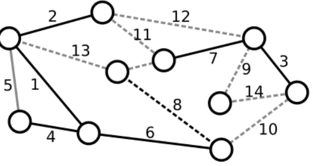
Figure 6.1: Snapshot of Kruskal’s algorithm. Solid black edges have been added toT, the solid gray edges have been discarded. The dashed black edge is being processed and will be added toT since it does not close a cycle; the dashed gray edges will be processed in later iterations.
6.2 Being Greedy: Kruskal’s Algorithm
Considering greedy strategies is always a good starting point. In the case of an MST, this means to always add the cheapest useful edge first! As closing cycles is pointless, this yields Kruskal’s algorithm, compare Figure 6.1:
Algorithm 13Kruskal’s algorithm (centralized version)
1: sortE in ascending order of weights; denote the result by (e1, . . . , e|E|)
2: T :=∅
3: fori= 1, . . . ,|E|do
4: if T∪ {ei}is a forestthen
5: T :=T∪ {ei}
6: end if
7: end for
8: return T
Lemma 6.3. If an edge is heaviest in a cycle, it is not in the MST. If all such edges are deleted, the MST remains. In particular, Kruskal’s algorithm computes the MST.
Proof. Denote the MST by M and suppose for contradiction that e ∈ M is heaviest in a cycleC. AsC\ {e} connects the endpoints ofe, there must be an edgee0 ∈Cso that (M\ {e})∪ {e0}is a spanning tree (i.e.,e0connects the two components ofM\ {e}). However, asW(e0)< W(e), (M\ {e})∪ {e0}is lighter thanM, contradicting thatM is the MST.
Thus, when deleting all edges that are heaviest in some cycle, no MST edge is deleted. As this makes sure that there is no cycle contained in the obtained edge set, the result is a forest. As this forest contains the MST, but a tree is a maximal forest, the forest must in fact be the MST.
Let’s make this into a distributed algorithm! Of course we don’t simply collect all edges and execute the algorithm locally. Still, we need to somehow collect the information to compare. We do this, but drop all edges which are certainly “unnecessary” on the fly.
Algorithm 14Kruskal’s algorithm (distributed version)
1: compute an (unweighted) BFS, its depth d, andn; denote the root byR
2: foreachv∈V in paralleldo
3: Ev :={{v, w} ∈E}
4: Sv:=∅// sent edges
5: end for
6: fori= 1, . . . , n+d−2 do
7: foreachv∈V \ {R} in paralleldo
8: e:= argmine0∈Ev\Sv{W(e0)} // lightest unsent edge
9: send (e, W(e)) tov’s parent in the BFS tree
10: Sv:=Sv∪ {e}
11: end for
12: foreachv∈V in paralleldo
13: foreach received (e, W(e))do
14: Ev :=Ev∪ {e}// also rememberW(e) for later use
15: end for
16: foreach cycleC inEv do
17: e:= argmaxe0∈C{W(e0)} // heaviest edge in cycle
18: Ev :=Ev\ {e}
19: end for
20: end for
21: end for
22: R broadcastsER over the BFS tree
23: return ER
Intuitively, MST edges will never be deleted, and MST edges can only be
“delayed,” i.e., stopped from moving towards the root, by other MST edges.
However, this is not precisely true: There may be other lighter edges that go first, as the respective senders do not know that they are not MST edges. The correct statement is that for the kth-lightest MST edge, at most k−1 lighter edges can keep it from propagating towards the root. Formalizing this intuition is a bit tricky.
Definition 6.4. Denote byBvthe subtree of the BFS tree rooted at nodev∈V, bydvits depth, byEBv :=S
w∈Bv{{w, u} ∈Ew}the set of edges known to some node in Bv, and by FBv ⊆EBv the lightest maximal forest that is a subset of EBv.
Lemma 6.5. For any node v and any E0 ⊆ EBv, the result of Algorithm 13 applied toE0 containsFBv∩E0.
Proof. By the same argument as for Lemma 6.3, Kruskal’s algorithm deletes exactly all edges from a given edge set that are heaviest in some cycle. FBv
is the set of edges that survive this procedure when it is applied to EBv, so FBv∩E0 survives for anyE0⊆EBv.
Lemma 6.6. For anyk∈ {0,1, . . . ,|FBv|}, afterdv+k−1rounds of the second FOR loop of the algorithm, the lightest k edges of FBv are in EBv, and have been sent to the parent by the end of round dv+k.
6.2. BEING GREEDY: KRUSKAL’S ALGORITHM 81 Proof. We prove the claim by double induction over the depthdvof the subtrees and k. The claim holds trivially true for dv = 0 and all k, as for leaves v we have EBv =FBv. Now consider v∈V and assume that the claim holds for all w∈V with dw < dv and allk. It is trivial fordv andk= 0, so assume it also holds fordv and somek∈ {0, . . . ,|FBv| −1}and consider indexk+ 1.
Because
EBv ={{v, w} ∈Ev} ∪ [
wchild ofv
EBw,
we have that the (k+ 1)th lightest edge in FBv is already known to v or it is inEBw for some childwofv. By the induction hypothesis for indexk+ 1 and dw< dv, each childwofv has sent thek+ 1 lightest edges inFBw tov by the end of round dw+k+ 1 ≤ dv+k. The (k+ 1)th lightest edge of FBv must be contained in these sent edges: Otherwise, we can take the sent edges (which are a forest) and edgesk+ 1, . . . ,|FBv| out of FBv to either obtain a cycle in which an edge fromFBv is heaviest or a forest with more edges than FBv, in both cases contained inEBv. In the former case, this contradicts Lemma 6.5, as then an edge fromFBv would be deleted fromE0⊆EBv. In the latter case, it contradicts the maximality of FBv, as all maximal forests in EBv have the same number of edges (the number of nodes minus the number of components of (G, EBv)). Either way, the assumption that the edge was not sent must be wrong, implying thatv learns of it at the latest in rounddv+kand adds it to Ev. By Lemma 6.5, it never deletes the edge fromEv. This shows the first part of the claim.
To show that by the end of the round dv+k+ 1, v sends the edge to its parent, we apply the induction hypothesis fordvandk. It shows thatv already sent the klightest edges from FBv before rounddv+k+ 1, and therefore will send the next in round dv+k+ 1 (or has already done so), unless there is a lighter unsent edge e ∈ Ev. As FBv is a maximal forest, FBv ∪ {e} contains exactly one cycle. However, as e does not close a cycle with the edges sent earlier, it does not close a cycle with all the edges inFBv that are lighter than e. Thus, the heaviest edge in the cycle is heavier thane, and deleting it results in a lighter maximal forest thanFBv, contradicting the definition ofFBv. This concludes the induction step and therefore the proof.
Theorem 6.7. For a suitable implementation, Algorithm 14 computes the MST M in O(n)rounds.
Proof. The algorithm is correct, if at the end of the second FOR loop, it holds that ER =M. To see this, observe that EBR =S
v∈V{{v, w} ∈E} =E and henceFBR=M. We apply Lemma 6.6 toRand roundn+d−2 =|M|+dR−1.
The lemma then says thatM ⊆ER. As in each iteration of the FOR loop, all cycles are eliminated fromER,ERis a forest. A forest has at most|M|=n−1 edges, so indeedER=M.
Now let us check the time complexity of the algorithm. From Lecture 2, we know that a BFS tree can be computed inO(D) rounds using messages of sizeO(logn).2 Computing the depth of the constructed tree and its number of nodesnis trivial using messages of sizeO(logn) andO(D) rounds. The second
2If there is no special nodeR, we may just pick the one with smallest identifier, start BFS constructions at all nodes concurrently, and let constructions for smaller identifiers “overwrite”
and stop those for larger identifiers.
FOR loop runs forn+d−1∈n+O(D) rounds. Finally, broadcasting then−1 edges of M over the BFS tree takes n+d−1 ∈n+O(D) rounds as well, as in each round, the root can broadcast another edge without causing congestion;
the last edge will have arrived at all leaves in round n−1 +d, as it is sent by R in roundn−1. As D≤n−1, all this takesO(n+D) =O(n) rounds.
Remarks:
• A clean and simple algorithm, and running time O(n) beats the trivial O(|E|) on most graphs.
• This running time is optimal up to constants on cycles. But (non-trivial) graphs with diameter Ω(n) are rather rare in practice. We shouldn’t stop here!
• Also nice: everyone learns about the entire MST.
• Of course, there’s no indication that we can’t be faster in case D n.
We’re not asking for everyone to learn the entire MST (which trivially would imply running time Ω(n) in the worst case), but only for nodes learning about their incident MST edges!
• To hope for better results, we need to make sure that we work concurrently in many places!
6.3 Greedy Mk II:
Gallager-Humblet-Spira (GHS)
In Kruskal’s algorithm, we dropped all edges that are heaviest in some cycle, because they cannot be in the MST. The remaining edges form the MST. In other words, picking an edge that cannot be heaviest in a cycle is always a correct choice.
Lemma 6.8. For any ∅ 6=U ⊂V, eU := argmin
e∈(U×V\U)∩E{W(e)} is in the MST.
Proof. As Gis connected, (U×V \U)∩E 6=∅. Consider any cycle C 3 eU. DenotingeU ={v, w},C\ {eU}connectsvandw. AseU ∈U×V\U, it follows that (C\ {eU})∩(U×V \U)6=∅, i.e., there is another edge e∈C between a node inU and a node inV\U besideseU. By definition ofeU,W(eU)< W(e).
As C 3eU was arbitrary, we conclude that there is no cycleC in whicheU is the heaviest edge. Therefore,eU is in the MST by Lemma 6.3.
This observation leads toanother canonical greedy algorithm for finding an MST. You may know the centralized version, Prim’s algorithm. Let’s state the distributed version right away.
Admittedly, this is a very high-level description, but it is much easier to understand the idea of the algorithm this way. It also makes proving correctness
6.3. GREEDY MK II: GALLAGER-HUMBLET-SPIRA (GHS) 83 Algorithm 15GHS (Gallager–Humblet–Spira)
1: T :=∅ //T will always be a forest
2: repeat
3: F := set of connectivity components ofT (i.e., maximal trees)
4: EachF ∈ F determines the lightest edge leavingF and adds it toT
5: untilT is a spanning subgraph (i.e., there is no outgoing edge)
6: return T
very simple, as we don’t have to show that the implementations of the individual steps work correctly (yet). We call an iteration of the REPEAT statement a phase.
Corollary 6.9. In each phase of the GHS algorithm, T is a forest consisting of MST edges. In particular, the algorithm returns the MST ofG.
Proof. It suffices to show thatT contains only MST edges. Consider any con- nectivity componentF ∈ F. As the algorithm has not terminated yet,Fcannot contain all nodes. Thus, Lemma 6.8 shows that the lightest outgoing edge ofF exists and is in the MST.
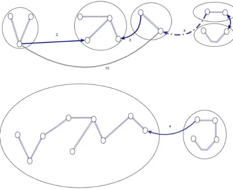
Figure 6.2: Two iterations of the GHS algorithm. The circled areas contain the components at the beginning of the iteration, connected by the already selected MST edges. Each component selects the lightest outgoing edge into the MST (blue solid arrows). Other edges within components, like the grey one after the first iteration, are discarded, as they are heaviest in some cycle.
Great! But now we have to figure out how to implement this idea efficiently.
It’s straightforward to see that we won’t get into big trouble due to having too many phases.
Lemma 6.10. Algorithm 15 terminates withindlognephases.
Proof. Denote bynithe number of nodes in the smallest connectivity component (maximal tree) in F at the end of phase i. We claim that ni ≥ min{2i, n}. Trivially, this number is n0 := 1 “at the end of phase 0,” i.e., before phase 1.
Hence, it suffices to show thatni≥min{2ni−1, n}for each phasei. To this end, consider anyF ∈ F at the beginning of phasei. UnlessF already contains all nodes, it adds its lightest outgoing edge toT, connecting it to at least one other component F0 ∈ F. As|F| ≥ni−1, |F0| ≥ni−1, and connectivity components are disjoint,|F∪F0| ≥2ni−1. The claim follows.
Ok, so what about the phases? We need to do everything concurrently, so we cannot just route all communication over a single BFS tree without potentially causing a lot of “congestion.” Let’s use the already selected edges instead!
Lemma 6.11. For a given phasei, denote byDi the maximum diameter of any F ∈ F at the beginning of the phase, i.e., after the new edges have been added toT. Then phasei can be implemented inO(Di)rounds.
Proof. All communication happens on edges ofT that are selected in or before phasei. Consider a connectivity component of T at the beginning of phasei.
By Corollary 6.9, it is a tree. We root each such tree at the node with small- est identifier and let each node of the tree learn this identifier, which takes O(d) time for a tree of depthd. Clearly, d ≤Di. Then each node learns the identifiers of the roots of all its neighbors’ trees (one round). On each tree, now the lightest outgoing edge can be determined by every node sending their lightest edge leaving its tree (alongside its weight) to the root; each node only forwards the lightest edge it knows about to the root. Completing this process and announcing the selected edges to their endpoints takesO(Di) rounds. As the communication was handled on each tree separately without using external edges (except for exchanging the root identifiers with neighbors and “marking”
newly selected edges), all this requires messages of sizeO(logn) only.
We’ve got all the pieces to complete the analysis of the GHS algorithm.
Theorem 6.12. Algorithm 15 computes the MST. It can be implemented in O(nlogn) rounds.
Proof. Correctness was shown in Corollary 6.9. As trivially Di ≤ n−1 for all phases i (a connectivity component cannot have larger diameter than the number of its nodes), by Lemma 6.3 each phase can be completed in O(n) rounds. This can be detected and made known to all nodes withinO(D)⊆ O(n) rounds using a BFS tree. By Lemma 6.10, there areO(logn) phases.
6.4. GREEDY MK III: GARAY-KUTTEN-PELEG (GKP) 85 Remarks:
• The lognfactor can be shaved off.
• The original GHS algorithm is asynchronous and has a message complex- ity of O(|E|logn), which can be improved to O(|E|+nlogn). It was celebrated for that, as this is way better than what comes from the use of an α-synchronizer. Basically, the constructed tree is used like a β- synchronizer to coordinate actions within connectivity components, and only the exchange of component identifiers is costly.
• The GHS algorithm can be applied in different ways. GHS for instance solves leader election in general graphs: once the tree is constructed, find- ing the minimum identifier using few messages is a piece of cake!
6.4 Greedy Mk III: Garay-Kutten-Peleg (GKP)
We now have two different greedy algorithms that run inO(n) rounds. How- ever, they do so for quite different reasons: The distributed version of Kruskal’s algorithm basically reduces the number of components by 1 per round (up to an additiveD), whereas the GHS algorithm cuts the number of remaining compo- nents down by a factor of 2 in each phase. The problem with the former is that initially there arencomponents, the problem with the latter is that components of large diameter take a long time to handle.
If we could use the GHS algorithm to reduce the number of components to something small, say√n, quickly without letting them get too big, maybe we can then finish the MST computation by Kruskal’s approach? Sounds good, except that it may happen that, in a single iteration of GHS, a huge component appears. We then wouldn’t know that it is so large without constructing a tree on it or collecting the new edges somewhere, but both could take too long!
The solution is to be more conservative with merges and apply a symmetry breaking mechanism: GKP grows components GHS-like until they reach a size of√
n. Every node learns its component identifier (i.e., the smallest ID in the component), and GKP then joins them using the pipelined MST construction (where nodes communicate edges between connected components instead of all incident edges).
Let’s start with correctness.
Lemma 6.13. Algorithm 16 adds only MST edges toT. It outputs the MST.
Proof. By Lemma 6.8, only MST edges are added toC in any iteration of the FOR loop, so at the end of the loopT is a subforest of the MST. The remaining MST edges thus must be between components, so contracting components and deleting loops does not delete any MST edges. The remaining MST edges are now just the MST of the constructed multigraph, and Kruskal’s algorithm works fine on (loop-free) multigraphs, too.
Also, we know that the second part will be fast if few components remain.
Corollary 6.14. Suppose after the FOR loop of Algorithm 16kcomponents of maximum diameterDmax remain, then the algorithm terminates withinO(D+ Dmax+k)additional rounds.
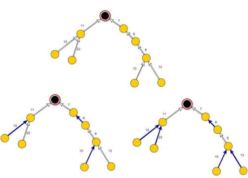
Figure 6.3: Top: A component of (F, C) in a phase of the first part of the GKP algorithm. “Large” components that marked no MST edge for possible inclusion can only be roots; we have such a root here. Bottom left: The blue edges show a matching constructed using the Cole-Vishkin algorithm. Bottom right: The blue edges are the final set of selected edges in this phase.
Algorithm 16 GKP (Garay–Kutten–Peleg). We slightly abuse notation by interpreting edges ofC also as edges between componentsF. Contracting an edge means to identify its endpoints, where the new node “inherits” the edges from the original nodes.
1: T :=∅ //T will always be a forest
2: fori= 0, . . . ,dlog√nedo
3: F := set of connectivity components ofT (i.e., maximal trees)
4: Each F ∈ F of diameter at most 2i determines the lightest edge leaving F and adds it to a candidate setC
5: Add a maximal matching CM ⊆Cin the graph (F, C) toT
6: IfF ∈ F of diameter at most 2i has no incident edge in CM, it adds the edge it selected intoC toT
7: end for
8: denote by G0 = (V, E0, W0) the multigraph obtained from contracting all edges ofT (deleting loops, keeping multiple edges)
9: run Algorithm 14 onG0 and add the respective edges toT
10: return T
Proof. The contracted graph has exactlyknodes and thusk−1 MST edges are left. The analysis of Algorithm 14 also applies to multigraphs, so (a suitable implementation) runs forO(D+k) additional rounds; all that is required is that
6.4. GREEDY MK III: GARAY-KUTTEN-PELEG (GKP) 87
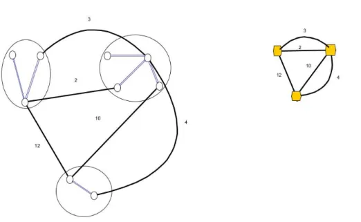
Figure 6.4: Left: Components and their interconnecting edges after the first stage of the GKP algorithm. Right: The multigraph resulting from contraction of the components.
the nodes of each component agree on an identifier for their component. This can be done by figuring out the smallest identifier in each component, which takesO(Dmax) rounds.
It remains to prove three things: (i) components don’t become too large during the FOR loop, (ii) we can efficiently implement the iterations in the FOR loop, and (iii) few components remain after the FOR loop. Let’s start with (i). We again call one iteration of the FOR loop a phase.
Lemma 6.15. At the end of phasei, components have diameterO(2i).
Proof. We claim that at the end of phasei, no component has diameter larger than 6·2i∈ O(2i), which we show by induction. Trivially, this holds for i= 0 (i.e., at the start of the algorithm). Hence, suppose it holds for all phases j≤i∈N0 for someiand consider phasei+ 1.
Consider the graph (F, C) from this phase. We claim that each component of the subgraph (F, C) induced by the selected edges has diameter at most 3.
To see this, observe that if an unmatchedF ∈ F adds an edge{F, F0},F0must be matched: otherwise,{F, F0} could be added to the matching, contradicting its maximality. Thus, all non-matching edges added toT “attach” someF ∈ F that was isolated in the graph (F, CM) to some F0 that is not picking a new edge in this step. This increases the diameter of components from at most 1 (for a matching) to at most 3.
Next, we claim that no component contains more than one F of diameter larger than 2i (with respect to G). This can be seen by directing all selected edges away from the F ∈ F that selected it (breaking ties arbitrarily). We obtain a directed graph of out-degree at most 1, in which any F of diameter
larger than 2i has out-degree 0 and is thus the root of a component that is an oriented tree.
Now consider a new component at the end of the phase. It is composed of at most one previous component of – by the induction hypothesis – size at most 6·2i, while all other previous components have size at most 2i. The longest possible path between any two nodes in the new component thus crosses the large previous component, up to 3 small previous components, and up to 3 edges between previous components, for a total of 6·2i+ 3·2i+ 3≤6·2i+1 hops.
Together with an old friend, we can exploit this to show (ii).
Corollary 6.16. Each iteration of the FOR loop can be implemented with run- ning time O(2ilog∗n).
Proof. By Lemma 6.15, in phase icomponents are of sizeO(2i). We can thus root them and determine the edges in C in O(2i) rounds. By orienting each edge in C away from the componentF ∈ F that selected it (breaking ties by identifiers), (F, C) becomes a directed graph with out-degree 1. We simulate the Cole-Vishkin algorithm on this graph to compute a 3-coloring inO(2ilog∗n) rounds. To this end, component F is represented by the root of its spanning tree and we exploit that it suffices to communicate only “in one direction,”
i.e., it suffices to determine the current color of the “parent.” Thus, for each component, only one color each needs to be sent and received, respectively, which can be done with message sizeO(logn) over the edges of the component.
The time for one iteration then is O(2i). By Theorem 1.7, we need O(log∗n) iterations; afterwards, we can select a matching inO(2i) time by going over the color classes sequentially (cf. Exercise 1) and complete the phase in additional O(2i) rounds, for a total ofO(2ilog∗n) rounds.
It remains to show that all this business really yields sufficiently few com- ponents.
Lemma 6.17. After the last phase, at most√ncomponents remain.
Proof. Observe that in each phasei, each component of diameter smaller than 2i is connected to at least one other component. We claim that this implies that after phase i, each component contains at least 2i nodes. This trivially holds for i= 0. Now suppose the claim holds for phasei∈ {0, . . . ,d√ne −1}. Consider a component of fewer than 2i+1 nodes at the beginning of phasei+ 1.
It will hence add an edge to C and be matched or add this edge to T. Either way, it gets connected to at least one other component. By the hypothesis, both components have at least 2inodes, so the resulting component has at least 2i+1. As there are dlog√nephases, in the end each component contains at least 2log√n=√nnodes. As components are disjoint, there can be at mostn/√n=
√ncomponents left.
Theorem 6.18. Algorithm 16 computes the MST and can be implemented such that it runs inO(√nlog∗n+O(D))rounds.
6.4. GREEDY MK III: GARAY-KUTTEN-PELEG (GKP) 89 Proof. Correctness is shown in Lemma 6.13. WithinO(D) rounds, a BFS can be constructed andnbe determined and made known to all nodes. By Corol- lary 6.16, phasei can be implemented inO(2ilog∗n) rounds, so in total
dlog√ ne
X
i=0
O(2ilog∗n) =O(2log√nlog∗n) =O(√
nlog∗n)
rounds are required. Note that since the time bound for each phase is known to all nodes, there is no need to coordinate when a phase starts; this can be com- puted from the depth of the BFS tree,n, and the round in which the root of the BFS tree initiates the main part of the computation. By Lemmas 6.15 and 6.17, only√ncomponents of diameterO(√n) remain. Hence, by Corollary 6.14, the algorithm terminates within additionalO(√n+D) rounds.
Remarks:
• The use of symmetry breaking might come as a big surprise in this al- gorithm. And it’s the only thing keeping it from being greedy all the way!
• Plenty of algorithms in the Congestmodel follow similar ideas. This is no accident: The techniques are fairly generic, and we will see next time that there is an inherent barrier around√n, even ifD is small!
• The time complexity can be reduced toO(p
nlog∗n+D) by using only llog(p
n/log∗n)m
phases, i.e., growing components to size Θ(p
n/log∗n).
• Be on your edge when seeing O-notation with multiple parameters. We typicallywant it to mean that no matter how the parameter combination is, the expression is an asymptotic bound where the constants in the O- notation areindependent of the parameter choice. However, in particular with lower bounds, this can become difficult, as there may be dependen- cies between parameters, or the constructions may apply only to certain parameter ranges.
What to take Home
• Studying sufficiently generic and general problems like MIS or MST makes sense even without an immediate application in sight. When I first encoun- tered the MST problem, I didn’t see the Cole-Vishkin symmetry breaking technique coming!
• If you’re looking for an algorithm and don’t know where to start, check greedy approaches first. Either you already end up with something non- trivial, or you see where it goes wrong and might be able to fix it!
• For global problems, it’s very typical to use global coordination via a BFS tree, and also “pipelining,” the technique of collecting and distributingk pieces of information inO(D+k) rounds using the tree.
Bibliographic Notes
Tarjan [Tar83] coined the terms red and blue edges for heaviest cycle-closing edges (which are not in the MST) and lightest edges in an edge cut3 (which are always in the MST), respectively. Kruskal’s algorithm [Kru56] and Prim’s algo- rithm [Pri57] are classics, which are based on eliminating red edges and selecting blue edges, respectively. The distributed variant of Kruskal’s algorithm shown today was introduced by Garay, Kutten, and Peleg [GKP98]; it was used in the first MST algorithm of running timeO(o(n) +D). The algorithm then was im- proved to running timeO(√nlog∗n+D) by introducing symmetry breaking to better control the growth of the MST components in the first phase [KP00] by Kutten and Peleg. The variant presented here uses a slightly simpler symmetry breaking mechanism. Algorithm 15 is called “GHS” after Gallager, Humblet, and Spira [GHS83]. The variant presented here is much simpler than the origi- nal, mainly because we assumed a synchronous system and did not care about the number of messages (only their size). As a historical note, the same princi- ple was discovered much earlier by Otakar Boruvka and published in 1926 – in Czech (see [NMN01] for an English translation).
Awerbuch improved the GHS algorithm to achieve (asynchronous) time com- plexityO(n) at message complexityO(|E|+nlogn), which is both asymptoti- cally optimal in the worst case [Awe87]. Yet, the time complexity is improved by the GKP algorithm! We know that this is not an issue of asynchrony vs.
synchrony, since we can make an asynchronous algorithm synchronous without losing time, using the α-synchronizer. This is not a contradiction, since the
“bad” examples have large diameter; the respective lower bound is existential. It says that for any algorithm, thereexists a graph with n nodes for which it must take Ω(n) time to complete. These graphs all have diameter Θ(n)! A lower bound has only the final word if it, e.g., says that for all graphs of diameter D, any algorithm must take Ω(D) time.4 Up to details, this can be shown by a slightly more careful reasoning than for Theorem 6.2. We’ll take a closer look at thep
nlog∗npart of the time bound next week!
Bibliography
[Awe87] B. Awerbuch. Optimal distributed algorithms for minimum weight spanning tree, counting, leader election, and related problems. In Proceedings of the nineteenth annual ACM symposium on Theory of computing, STOC ’87, pages 230–240, New York, NY, USA, 1987.
ACM.
[GHS83] R. G. Gallager, P. A. Humblet, and P. M. Spira. Distributed Algo- rithm for Minimum-Weight Spanning Trees. ACM Transactions on Programming Languages and Systems, 5(1):66–77, January 1983.
[GKP98] Juan A Garay, Shay Kutten, and David Peleg. A sublinear time dis- tributed algorithm for minimum-weight spanning trees. SIAM Jour- nal on Computing, 27(1):302–316, 1998.
3An edge cut is the set of edges (U×V \U)∩Efor some∅ 6=U⊂V.
4Until we start playing with the model, that is.
BIBLIOGRAPHY 91 [KP00] Shay Kutten and David Peleg. Fast Distributed Construction of Small
k-Dominating Sets and Applications, 2000.
[Kru56] Jr. Kruskal, Joseph B. On the Shortest Spanning Subtree of a Graph and the Traveling Salesman Problem. Proceedings of the American Mathematical Society, 7(1):48–50, 1956.
[NMN01] Jaroslav Neˇsetˇril, Eva Milkov´a, and Helena Neˇsetˇrilov´a. Otakar Boru- vka on Minimum Spanning Tree Problem Translation of Both the 1926 Papers, Comments, History.Discrete Mathemetics, 233(1–3):3–
36, 2001.
[Pri57] R. C. Prim. Shortest Connection Networks and some Generalizations.
The Bell Systems Technical Journal, 36(6):1389–1401, 1957.
[Tar83] Robert Endre Tarjan.Data Structures and Network Algorithms, chap- ter 6. Society for Industrial and Applied Mathematics, Philadelphia, PA, USA, 1983.