Molecular dynamics simulations of graphene-based polymer nanocomposites

(1)

Book Chapter

Molecular dynamics simulations of graphene-based polymer nanocomposites

Author(s):

Skountzos, Emmanuel N.; Mavrantzas, Vlasios Publication Date:

2020-04

Permanent Link:

https://doi.org/10.3929/ethz-b-000455792

Originally published in:

http://doi.org/10.1515/9783110479133-005

Rights / License:

Creative Commons Attribution-NonCommercial-NoDerivatives 4.0 International

This page was generated automatically upon download from the ETH Zurich Research Collection. For more information please consult the Terms of use.

ETH Library

(2)

graphene-based polymer nanocomposites

5.1 Introduction

5.1.1 Carbon-based materials – the case of graphene

During the last decades, carbon has attracted a great deal of scientific and indus- trial attention due to the discovery of several allotropes (graphene, fullerene, carbon nanotubes [CNTs]), which are characterized by unprecedented physical and chemical properties such as high mechanical strength, extremely high electrical and thermal conductivity, high optical transparency and excellent gas barrier properties. Because of these unique features, carbon materials are widely used as nano- fillers for the fabrication of composite materials with applications in several fields (biology, energy storage, transport and aviation, optoelectronics, pharmaceutics, medicine and many others). Fullerenes, for example, are used as electron acceptors for the fabrication of organic solar cells based on semiconducting polymers such as poly-3-hexyl thiophene, which has significantly improved the efficiency of the corresponding devices, reaching values comparable to those of inorganic solar cells.

Graphene-based biosensors characterized by remarkable detection efficiency toward certain target molecules have also been manufactured by exploiting the excellent electrical and optical properties of graphene even when present at very low concentrations. The very high specific surface area of CNTs combined with their low electrical resistance and high charge transport capability have allowed the production of high-performance supercapacitors with increased energy storage, power- delivery capabilities and rather long-life cycle compared to conventional batteries.

From the broad family of the carbon-based nanoparticles (NPs), the one that has attracted the most significant attention is graphene, a one-atom-thick planar sheet of sp2-bonded carbon atoms densely packed in a honeycomb crystal lattice.

Graphene is the basic building block for graphitic materials of all other dimension- alities (Figure 5.1), because it can be wrapped up into 0D fullerenes, rolled into 1D nanotubes or stacked into 3D graphite [1].

Emmanuel N. Skountzos,Department of Chemical Engineering, University of Patras, Patras, Greece; Foundation of Research and Technology Hellas, Institute of Chemical Engineering Sciences (FORTH/ICE-HT), Rio-Patras, Greece

Vlasis G. Mavrantzas,Department of Chemical Engineering, University of Patras, Patras, Greece;

Foundation of Research and Technology Hellas, Institute of Chemical Engineering Sciences (FORTH/ICE-HT), Rio-Patras, Greece; Particle Technology Laboratory, Department of Mechanical and Process Engineering, ETH Zürich, Switzerland

This work is licensed under a Creative Commons Attribution-NonCommercial-NoDerivatives 4.0 International License.

https://doi.org/10.1515/9783110479133-005

(3)

Until 2004, the production of single-layer (SL) graphene sheets (GS) was considered impossible, since theoretical calculations had predicted that GS would be completely unstable. The successful isolation of SL, defect-free GS using the“scotch tape method”[2] led to a rapid expansion of the field. The discovery was made by Prof. Sir Kostya Novoselov and Prof. Sir Andre Geim, who were awarded the Nobel Prize in Physics in 2010.

The impact of graphene on the scientific community has been enormous.

Thousands of scientific articles (experimental and theoretical) are published every year and hundreds of these are heavily cited, while the paper describing the simple method to produce perfect GS has been characterized as“one of the most cited recent papers in the field of Physics” according to the ISI citation index. Apart from the great scientific interest in this exotic material, a significant impact on the largest technological industries of the world has also emerged after its discovery. Every year, thousands of patents are filed around the world on the design of new materials and new devices with important implications for practically all aspects of modern life (medicine, transportation, electronics, etc.), which explains why graphene has been characterized as the material of the future.

5.1.2 Graphene and graphene-based polymer nanocomposites

Numerous excellent reviews have been written in the last few years on the production, properties and applications of graphene [3–7] and graphene-based nanocomposites [8–13]; hence, here we will limit ourselves only to a brief overview of its

Figure 5.1:Graphene, the building block of all graphitic forms.

(4)

unique structural and physicochemical properties, and for more details we refer the interested reader to the original articles.

Production of graphene

After a long and tenacious series of unsuccessful attempts to produce SL graphene, the publication of a simple method was presented in 2004 [2] known today as the

“scotch tape method.”By repeatedly cleaving a graphite crystal flake with an adhe- sive tape to its limit, and then transferring the thinned-down graphite onto an oxi- dized silicon wafer with the appropriate color, a 2D carbon lattice is produced.

In general, production methods of graphene fall into two main categories:

– Bottom-up methods – Top-down methods

In bottom-up processes, graphene is synthesized by a variety of methods such as 1. Epitaxial growth on metal carbides [14–16]

2. Chemical vapor deposition (CVD) [17–18]

3. Unzipping CNTs [19–20]

In top-down processes, it is synthesized from a bulk material (e.g., graphite), which is broken down into smaller pieces using mechanical, chemical or other forms of energy. Typical examples of the top-down production processes include

1. the micromechanical exfoliation of graphite [2];

2. the direct sonication of graphite [21–22];

3. the chemical reduction of organically treated graphite oxide [23] and 4. the thermal exfoliation/reduction of graphite oxide [24].

In principle, with bottom-up approaches, large-sized, defect-free monolayer graphene is produced, a perfect material for the subsequent studies. The only drawback with these methods is that they afford only the production of tiny amounts of graphene. Top-down processes, on the other hand, are suitable for the large-scale production of graphene as (for example) required for the fabrication of graphene- based polymer nanocomposites.

Properties of graphene

The rapid adoption of graphene as the material of interest lies primarily in the excellent spectrum of properties (mechanical, electrical, thermal, optical, etc.) charac- terizing monolayer, few-layer graphene and graphene oxide (GO). The goal of many research efforts nowadays is to exploit these extraordinary properties for applications

(5)

in nanotechnology by fabricating materials with improved mechanical, electrical, thermal and optical performance.

Carbon-based nanomaterials such as graphite, diamond and CNTs have their own record in terms of mechanical strength, hardness or Young’s modulus. The newest member of the family, graphene, is no exception despite that its mechanical behavior has not been investigated as much as its electronic and optical properties.

The reported stiffness of about 300–400 N/m (with a breaking strength of about 42 N/m) represents the intrinsic strength of a defect-free sheet [25] while estimates of the Young’s modulus are on the order of 0.5–1.0 TPa [25]. Interestingly, and despite their defects, suspended GO sheets retain to a large extent their mechanical performance, characterized by a Young’s modulus of 0.25 TPa [26]. These features, combined with the relatively low cost for the production of thin graphite and the ease of processes for blending GO into matrices [11], render these materials as ideal candidates for electrical and mechanical reinforcement [27, 28].

Regarding electrical properties of graphene, we mention that its electrical resistivity at room temperature is about 1μΩcm; as a result, graphene is about 35% less resistant than silver, the lowest resistivity material known today at room temperature. In semiconductors, a different measure is used to quantify electronic motion known as mobility. Mobility is often expressed as the conductivity of the material per electronic charge carrier. This implies that high mobility is advantageous also for chemical or biochemical sensing applications in which a charge signal (e.g., a molecule adsorbed on a device) is translated into an electrical signal, thanks to the changing conductivity of the device. Thermal vibrations of atoms set the upper limit to electron mobility in graphene, which is ~200,000 cm²/V s [29–30] at room temperature, which should be compared to ~100,000 cm²/V s [31] in CNTs.

Chen et al. [32–33] showed that although the room temperature limit of mobility in graphene can be as high as 200,000 cm²/V s, in present-day samples the actual mobility is lower (around 10,000 cm²/V s) leaving significant room for improvement. Because graphene is only one-atom thick, current samples must be supported by a substrate, typically silicon dioxide. Trapped electrical charges in silicon dioxide (a sort of atomic-scale dirt) can interact with electrons in graphene, which can cause a reduction in mobility.

In addition to being considered as a promising material for applications in chemical and biochemical sensing, its low resistivity and extremely thin nature render graphene a very promising material also for use in thin, mechanically tough, electrically conducting, transparent films that are needed in many applications in electronics (ranging from touch screens to photovoltaic cells).

Apart from its excellent mechanical and electrical properties, graphene exhibits amazing performance as a thermal conductor. Balandin et al. [34] reported values of thermal conductivity for SL graphene at room temperature in the range of 4,840–5,300 W/m K. These extremely high values of thermal conductivity suggest that graphene can outperform CNTs in heat conduction [35–36]. However, when

(6)

graphene is in contact with a substrate, its thermal transport properties can be significantly affected. Seol et al. [37] showed experimentally that the value of thermal conductivity of monolayer graphene exfoliated on a silicon dioxide support is still as high as about 600 W/m K near room temperature, exceeding those of metals such as copper. It is lower, however, than that of suspended graphene because of phonons leaking across the graphene–support interface and strong interface scat- tering of flexural modes, which make a large contribution to thermal conductivity for suspended graphene. In general, the superb thermal conduction properties of graphene have established it as an excellent material for thermal management.

Production of graphene-based polymer nanocomposites

In recent years, a variety of processing methods have been proposed for dispersing GS into polymer matrices. Many of these procedures are like those used for other nanocomposite systems (e.g., CNT/polymer nanocomposites) [38], while others apply only to graphene-based polymer nanocomposites.

A crucial step in the production of any polymer nanocomposite is the dispersion of the nanofiller. A well-dispersed state ensures a maximized reinforced surface area, which directly affects all properties of the nanocomposite. Efforts are therefore focused on achieving a well-dispersed, homogeneous system by developing either covalent or noncovalent functionalization of the filler surface, an issue that will be discussed in some more detail in the following sections.

Most polymer/graphene composites are produced today with one of the following three strategies: (1) solvent processing, (2) in situ polymerization and (3) melt processing with each one of them having its own advantages and disadvantages. In the solvent processing method, GS are initially dispersed in a suitable solvent, a procedure typically assisted by ultrasonication [11, 39]. Then, the polymer is added in the solvent/graphene blend, and the solvent is finally removed by evaporation or distillation. It is a rather simple method, used widely to prepare polymer/graphene composites. Its most important drawback is that common organic solvents adsorb on GS stronger than most of the polymers.

In the in situ polymerization method, GS are mixed with the targeted mono- mers, and by adjusting parameters (such as temperature and pressure), the polymerization reaction proceeds [40–41]. The advantages of the method are twofold:

(a) it provides a strong interaction between the polymer matrix and the surface of GS and (b) it leads to highly homogeneous dispersions. However, an increase in the viscosity of the blend is usually recorded as a side effect, which affects processabil- ity (especially at high GS loadings).

Melt processing is commercially the most attractive method to produce graphene-based polymer composites. It involves the direct inclusion of GS into the melted polymer using a twin-screw extruder by suitably adjusting parameters such

(7)

as screw speed, temperature and time [42–43]. Drawbacks of the method include the low density of thermally exfoliated graphene that makes extruder feeding a troublesome task, and the lower degree of dispersion achieved compared to solvent blending. Reduced degree of dispersion typically results in poorer mechanical, electrical and thermal properties.

Properties of graphene-based polymer nanocomposites

In the modern literature, significant improvements in the mechanical, electrical, thermal and barrier properties of graphene-based polymer nanocomposites have been reported, as summarized in several reviews [8–10, 12, 44]. Fang et al. [40], for example, have reported an increase in the tensile strength by 70% and in the Young’s modulus by 57% for graphene–polystyrene nanocomposites with polystyrene (PS) chains grafted onto GS by atomic transfer radical polymerization. The experimental studies of Ramanathan et al. [39] and Li and McKenna [45] have shown that behind the extraordinary mechanical properties and the increase in the glass transition temperature (T_g) of poly(methyl methacrylate) (PMMA) nanocomposites filled with functionalized graphene sheets (FGS) are the enhanced interfacial interactions with PMMA chains as driven by oxygen functionalities across the surface of graphene. FGS contain pendant epoxy, hydroxy and/or carboxy groups on their surface, which may form hydrogen bonds with the ester branches of PMMA. However, Liao and coworkers [46–47] have argued that an 80% increase in the PMMA modulus [39] at only 1 wt. % loading of the nanocomposite in FGS, and an increase inT_gby 29 °C [39] at only 0.05 wt.% loading seem unrealistically high. Thus, Liao et al. repeated the experiments carried out by Ramanathan et al. [39] and found an increase of only 25% in the Young’s modulus measured [47] and no change in theT_g[46]. These very different observations were attributed to the experimental procedure followed by Ramanathan et al. [39]. In an earlier study [48], significant improvements in the Young’s modulus and in ul- timate tensile strength had been reported for poly(vinyl alcohol) (PVA) samples enhanced with GO sheets functionalized with PVA chains (PVA chains had been grafted onto the GO surface). The reported enhancement in the mechanical performance reached almost 60% for GO loadings below 0.3 vol.% [48]. For the same nanocomposite, Zhao et al. [49] have reported an improvement of ~150% in the tensile strength and an order of magnitude increase in the Young’s modulus for only a 1.8 vol.% loading in graphene.

As already mentioned, graphene-based materials are very promising for the development of new devices with applications in electronics, owing to their high degree of electrical conductivity. In the past, several carbon-based NPs (i.e., carbon filler, carbon nanofibers, expanded graphite, etc.) have been exploited for the production of electrically conductive composites; however, the key advantage of graphene is that the insulator-to-conductor transition (known as the percolation threshold) can

(8)

be achieved at significantly lower loadings. Production of electrically conductive polymers has been reported [50–51] upon successful GS dispersion in the host polymer matrix. Stankovich et al. [11, 52] determined the percolation threshold for a polystyrene solvent blended with GO to be 0.1 vol.%, perhaps the lowest percolation threshold ever reported. Eda and Chhowalla [53] studied the electrical properties of solution-processed, semiconducting thin films consisting of FGS as the filler and polystyrene as the host material and found that upon increasing the average size of FGS significantly enhanced carrier mobility and thus device performance. This study demonstrated how a commodity plastic can be used to develop low-cost, macroscale thin-film electronics.

Simulations

In addition to experimental efforts, theoretical and computational works have addressed several aspects of the structure–property–processing relationship in graphene or graphene-based nanocomposite materials. Several simulation techniques and approaches have been employed, extending from the quantum level to the atomistic to the mesoscopic and finally to the macroscopic. The findings of these theoretical studies have significantly improved our understanding of the microscopic mechanisms and interactions governing the macroscopically exhibited properties of these new classes of materials.

Using classical ab initio calculations, Van Lier et al. [54] and Liu et al. [55] reported values of graphene’s Young’s modulus equal to 1.11 and 1.05 TPa, respectively, which are in reasonable agreement with the experimentally measured ones [25]. It is worth mentioning that the computational values were reported in 2000 [54] and 2007 [55], respectively, while the experimental one in 2008 [25]. In a recent study that combined density functional theory calculations and classical molecular dynamics (MD) simulations, Kalosakas and coworkers [56] proposed a new force field specifically for graphene that takes into account only bond stretching (described by a Morse-style potential) and bond bending (described by a nonlinear function containing quadratic and cubic terms) interactions between carbon atoms.

The new potential was employed in simulations with model graphene systems subject to uniaxial tension or to hydrostatic compression, yielding a value of 0.95 TPa [56] for graphene’s Young’s modulus, which is also consistent with the one measured experimentally [25]. The dependence of graphene’s Young’s modulus on temperature and size of GS was systematically studied by Jiang et al. [57], through MD deformation simulations of SL graphene using progressively larger GS, and an increase in the Young’s modulus was observed with increasing GS size. The plateau value was reached for a GS size equal to 25 Å × 25 Å beyond which no further increase was recorded [57]. The MD deformation experiments were carried out at temperatures ranging from 100 to 600 K; a slight increase in the value of the Young’s

(9)

modulus (within the statistical error) was monitored for temperatures up to 500 K, followed by a rapid decrease at higher temperatures.

Ab initio studies of suspended GS are not restricted solely to the estimation of the mechanical properties. Excellent articles have been reported in the literature ad- dressing atom–atom interactions between graphene and popular substrates (e.g., SiC [58]καιMoS2[59]) that are extensively used for the fabrication of SL graphene. Also important are computational and simulation studies of the mechanical, thermal, barrier and electronic properties of polymers filled with GS. Issues addressed here include microscopic structure, chain conformation and local and terminal dynamics of polymer matrix chains in the presence of graphene. Earlier works focused on the study of the interfacial behavior of graphene-based polymer composites. Awasthi and coworkers [60] carried out atomistic MD simulations with the consistent valence force field to study nanoscale load transfer between polyethylene (PE) and GS and characterize the force-separation behavior between CNTs and a polymer matrix.

Separation studies were conducted for opening and sliding modes, and cohesive zone parameters (such as the peak traction and the energy of separation for each mode) were evaluated as a first step toward the development of continuum length- scale micromechanical models for tracking the overall material response by incorporating information about the underlying interfacial interactions. MD simulations have also been employed by Li et al. [61] in their study on the effect of the shape of carbon-based NPs on the viscoelastic properties of a PE matrix. They found that it is the surface-to-volume ratio of the NPs that plays the most important role in the structural, dynamical and viscous properties [61]. More recent MD simulations [62–63] of PMMA/graphene nanocomposite showed strong adhesion of PMMA chains (especially of the side groups) on graphene, and considerably slower segmental and chain mobility in the interfacial area. The MD simulations suggest that local mass density, segmental dynamics and chain terminal relaxation all differ from the bulk behavior up to distances equal to several nanometers from the GS surface. Very similar results have been reported for a different matrix, PE [64], demonstrating large density inho- mogeneities due to strong PE chain adsorption on the surfaces of GS, exactly as was reported in the case of PMMA/graphene nanocomposites [62]. Close to graphene, PE chains prefer to stand parallel to the graphene surface [64], and all polymer conformational and dynamic properties [64–65] are significantly affected: (a) the size of polymer chains (as measured by their radius of gyration) increases and (b) their dynamics change dramatically because their orientational relaxation time increases almost by one order of magnitude compared to the bulk value. In a very recent work [66], the effect of GS on the crystallization process of PE, polyvinylidene fluoride (PVDF) and PS oligomers was examined. It was reported that GS tend to act as nucle- ation sites for the crystallization of PE and PVDF but not for PS, which remains almost amorphous [66]. It was also reported that at high temperatures (e.g., close to 600 K), the crystalline structure of PE is destroyed, a result that is in accordance with the recent MD study of Gulde et al. [67].

(10)

Simulations have also addressed polymer nanocomposites enhanced not with pristine GS but with GO. GO is graphene-bearing epoxy, hydroxy and/or carboxy groups on its surface. When GO is used as a nanofiller of a polar (e.g., acrylic) polymer, the interactions between polymer atoms and graphene are intensified due to strong attractive forces that develop between polymer and GO oxygen atoms. Lv et al. [68] examined two different polymers as the host matrix, PMMA and PE, and concluded that with increasing concentration in carboxyl content, the interaction energy between polymer chains and GO sheets decreased (it became more attractive), followed by a significant increase in the value of the shear stress. However, an upper bound in the concentration was found, beyond which no further change in the values of these two properties was observed. This was explained as a satura- tion effect: high concentrations of functional groups strengthen the interactions between the surface functionalization groups themselves, thus no space is left for interactions with the surrounding polymer chains. Karatasos and Kritikos [69] have reported a strong increase (by 38 °C) of theT_gof GO-based poly(acrylic acid) (PAA) nanocomposites compared to pure polymer (PAA). This strong increase was explained by the strong adsorption of PAA chains onto the surface of GO sheets facili- tated by the hydrogen bonds that develop between the hydroxyl groups of GO and the oxygen atoms of PAA branches. Earlier, Xue et al. [70] had studied theT_gof PMMA matrices enhanced either with pristine GS or with GS modified with -COOH and -NH₂groups. By employing classical MD simulations, they observed a 30 °C increase in theTgof the PMMA/GS system, whereas for the nanocomposites with the modified GS, the shift was higher (40 °C) [70]. More recently, Azimi et al. [71]

showed that the dynamics of a polar (e.g., PVA) matrix is affected more by the presence of GO than by the presence of GS, whereas for an apolar polymer matrix (e.g., poly(propylene)) the effect of the two types of graphene is almost the same. That less polymer is adsorbed on GO than on pristine graphene can be explained by the roughness of GO particles due to OH- and -O- groups on their surface and agrees with a recent detailed MD study by Skountzos et al. [72]. However, the strength of interactions between oxygen atoms of the polar polymer and of GO particles is so strong that despite the smaller adsorbed amount on GO (in comparison to pristine GS), the dynamics of the PVA/GO system is considerably slower than the dynamics of the PS/GS nanocomposite.

In the last years, significant progress has been made in predicting the unique mechanical properties of graphene-based polymer nanocomposites through detailed atomistic-level simulations and understanding the underlying molecular mechanisms behind these properties [55, 72–76]. A typical example is the atomistic simulation work of Skountzos et al. [72] on the effect of pristine graphene and GO on the structure, conformation and mechanical properties of a syndiotactic PMMA (sPMMA) matrix. The atomistic simulations predicted a significant enhancement of all elastic constants (Young’s, shear and bulk moduli and Poisson’s ratio), especially for the PMMA/GO nanocomposites, which was attributed to the hydrogen

(11)

bonds that develop between the oxygen atoms at the branches of PMMA chains and the OH- and -O- groups on the surface of GO particles. Wang et al. [76] have studied the effect of surface functionalization and graphene size on the interfacial load transfer in graphene–PE nanocomposites (by employing the ab initio polymer- consistent force field, PCFF) and showed that oxygen-FGS lead to larger interfacial shear force (than hydrogen-functionalized or pristine ones) during the pull-out process. Increasing the oxygen coverage and graphene size enhanced the interfacial shear force, but further increasing the oxygen coverage to about 7% led to a satura- tion in the interfacial shear force. Liu et al. [75] studied the effect of shape of carbon-based NPs on the toughening efficiency of a PE matrix by applying pure tensile strain experiments in MD simulations with several model systems. At the same wt.

% loading in either CNTs, or fullerenes or GS, they found that the highest toughening was observed for the PE/graphene system; this should be related to the increased surface area that graphene offers for PE chain adsorption. This effect was examined in both the rubbery and glassy states (i.e., above and below the glass transition temperature of PE) and it was found that the nanocomposite in the rubbery state was tougher than the corresponding glassy material [75]. More recently, in a systematic study, Lin et al. [73] investigated how temperature and GS loading affect the mechanical performance of model PMMA/GS nanocomposites. The general trend was that Young’s and shear moduli increase with increasing GS loading but decrease with increasing temperature while the temperature dependence of the two moduli is stronger in the nanocomposites with the higher concentration in GS.

Comparison of their simulation results with the equations based on the simple rule of mixing for the mechanical properties of microfiber-reinforced composites re- vealed that the latter do not apply for graphene-reinforced nanocomposites; thus, further research is needed to address this issue [73].

Graphene dispersion

Clearly, among all NPs considered as polymer reinforcing agents, graphene is the most promising due to its outstanding features. However, because of its high specific surface area and tendency for self-adhesion (driven by the very strong van der Waals forces andπ–π interactions), GS tend to agglomerate in the form of multi- layer graphitic structures. Significant research has thus been undertaken in the last years to understand and improve GS dispersion, and thus realize its unique properties in practice. The degree of GS dispersion in nanocomposites affects primarily their mechanical performance. Indeed, several studies have shown that the mechanical properties of graphene-based polymer nanocomposites increase as their content in SL graphene increases [39, 77–78]. Motivated by these findings, in the next paragraphs of this chapter we provide a brief overview of the methods employed

(12)

nowadays, typically based on covalent or noncovalent graphene functionalization, to achieve homogeneous GS dispersions [79–80].

Techniques based on covalent functionalization make use of small molecules or entire macromolecules that are attached on the surface of GS through covalent bonding. Then, owing to strong chemical interactions developing between the grafted groups and the GS, very homogeneous and stable dispersions can be obtained. However, covalent functionalization disrupts the perfect crystal structure of graphene, which can affect many of its outstanding properties, especially the electrical ones. An attractive alternative is noncovalent functionalization. This is based on the use of functional groups that are attached on the surface of graphene through favor- ableπ–πinteractions without disturbing its electronic network. Noncovalent methods are by default nondestructive; however, the forces that develop between the wrapping molecules and the graphene surface are much weaker compared to those in the case of covalent functionalization; this can limit the degree of dispersion eventually achieved.

Covalent functionalization of graphene has been exploited quite widely in the literature for the improvement of the mechanical properties of graphene-based nanocomposites [81–85]. Using mostly peripheral ester linkages that are extensively used in tissue engineering applications, Sayyar et al. [84] managed to successfully link polycar- bonate to GO. The fabricated nanocomposite had a very homogeneous and stable GS dispersion and exhibited several good properties: improved Young’s modulus, improved tensile strength and high electrical conductivity (~14 orders of magnitude compared to the conductivity of the pure bulk polymer). In an earlier study, Cheng and coworkers [81] had produced PVA nanocomposites by incorporating PVA-grafted GO fillers, which resulted in an enhancement of Young’s modulus by 150% and of tensile strength by 88%, for 1 wt.% loading of the nanocomposite in GO.

The tendency of GS to agglomerate and form graphitic structures is witnessed most easily in atomistic or coarse-grained simulations. Park and Aluru [86] have reported GS self-assembly in atomistic MD simulations of GS in water solutions, but this was probably an expected result due to hydrophobic nature of graphene. In a later study, Li and coworkers [61] found that several carbon allotropes (buckyballs, graphe- nes, etc.) agglomerate in a PE matrix, thus lowering the degree of their interaction (con- tacts) with the host matrix. Ju et al. [87] studied the degree of GS miscibility in PMMA as a function of NP volume fraction with the help of dissipative particle dynamics (DPD) simulations using different values of the DPD-repulsive interaction parameter to effectively account for surface functionalization. GS agglomeration has also been reported by Karatasos et al. [88–89] in all-atom MD simulations of linear and hyper- branched polymer matrices. Guo et al. [90] have studied the effect of GS agglomeration on the mechanical properties of polymer nanocomposites by examining cases where several GS were intercalated (polymer chains were“sandwiched”between two consecutive GS) or stacked (in the form of graphite-like structure) in the sample. By investi- gating their mechanical behavior in a series of uniaxial tension experiments, they concluded that intercalated systems exhibit a higher storage modulus compared to

(13)

stacked ones due to stronger interactions between the polymer and the GS resulting from the higher surface-to-volume ratio in the intercalated design. More recently [91], atomistic MD simulations were combined with advanced chemistry techniques to produce graphene-based PMMA solutions and nanocomposites of high degree of GS dispersion. Instead of graphene covalent functionalization or incorporation of small molecules as dispersing agents in the solutions, in the new method a fraction of PMMA chains were covalently functionalized by a procedure that allows adding pyrene molecules preferentially to the two ends of the polymer chain [91]. The accompanying MD simulations provided very useful information about the interaction of these functionalized PMMA chains with GS and how these are kept well separated in the polymer matrix, thereby achieving a stable, highly homogeneous dispersion.

5.2 Simulation methods at the atomistic level:

the molecular dynamics method

In the last few decades, molecular simulations have emerged as an excellent tool for explaining many of the microscopic mechanisms behind the measured macroscopic properties of complex materials, also for connecting the predictions of theoretical models with experimentally measured properties. Being able, in particular, to predict important material properties from the chemical composition and molecular architecture of the chemical formulation is of paramount importance because it can guide design efforts both at the level of materials synthesis and at the level of materials processing. With their inherent potential to predict important physical properties directly from the underlying atomistic structure, molecular simulations are considered today as very useful, virtual experiments that can replace in many cases actual laboratory measurements.

Molecular simulations encompass two main techniques: MD and Monte Carlo (MC) [92–93]. MD is based on the solution of Newton’s equations of motion in an appropriate statistical ensemble. These are numerically integrated, and the result of integration yields the positions and velocities of each atomistic unit in the system in time (this is also known as the trajectory of the system in phase space). In this way, we can monitor how the model system involves in time (under the macroscopic constraints imposed by the statistical ensemble in which the simulation is carried out) and thus extract information about its thermodynamic, structural, conformational, dynamic and rheological properties. To run an MD simulation, we need initial conditions, namely atomic positions and atomic velocities at zero time.

The trajectory followed by the system depends then crucially on the potential energy function describing intra- and intermolecular interactions.

In contrast to MD which is a deterministic method, MC is based on the design of (artificial or even unphysical) moves to sample new states that are selected

(14)

randomly with the help of an appropriate acceptance criterion. Thanks, in particular, to the design of some very clever moves, MC helps the system tunnel through large potential energy barriers, and this can accelerate system equilibration by orders of magnitude compared to MD. The major drawback of the method is that it does not offer any dynamic information about the system. This happens because the system evolves stochastically in configuration space based on predefined acceptance criterion for each attempted move. Indeed, in a MC simulation, only atomic positions matter. Our discussion in the remainder of this chapter is devoted solely to the MD method.

In general, the complexity of polymers prohibits the analytical solution of the corresponding statisticomechanical problem. Molecular simulations overcome this by solving the corresponding problem numerically, given a mathematical model for the molecular geometry and description of interatomic interactions. Two general types of force fields are typically employed for the molecular simulation of polymers: Explicit atom (EA) models where every atom is considered as an independent interaction site or entity, and united atom (UA) models where hydrogen atoms are neglected by considering a relatively larger, spherically interacting particle that em- bodies the contributions of both the hydrogen atoms and of the atom (e.g., the carbon) to which the hydrogens are bonded. EA models offer a very detailed and accurate description of the problem. Their main drawback is that, for the same number of total molecules considered in the simulation box, they involve almost twice as many interacting sites as the corresponding UA model; as a result, molecular simulations with EA models are significantly more CPU time demanding than simulations with UA models.

Given the type of molecular model adopted, an initial configuration for the system and initial velocities for all atoms (assigned according to the Maxwell–Boltzmann distribution), what remains to be defined next is the potential energy function describing interatomic interactions. In general, these are distinguished between bonded and nonbonded. Bonded interactions typically include contributions from

– bond length stretching (Figure 5.2a), – bond angle bending (Figure 5.2b), – proper dihedral angles (Figure 5.2c) and – improper dihedral angles (Figure 5.2d).

Nonbonded interactions, on the other hand, include

– inter- and intramolecular van der Waals interactions (Figure 5.2e) and – inter- and intramolecular Coulomb interactions (Figure 5.2f).

(15)

A typical mathematical form of the total potential energy function [94] is

Upot=X

bonds

k_bðb−b0Þ²+X

angles

k_θðθ−θ⁰Þ²+ X

dihedrals

k_ϕ½1+cosðn’−δÞ+ X

impropers

k_χðχ−χ0Þ² zfflfflfflfflfflfflfflfflfflfflfflfflfflfflfflfflfflfflfflfflfflfflfflfflfflfflfflfflfflfflfflfflfflfflfflfflfflfflfflfflfflfflfflfflfflfflfflfflfflfflfflfflfflfflfflfflfflfflfflfflfflfflfflfflfflfflfflfflfflfflfflfflfflfflfflffl}|fflfflfflfflfflfflfflfflfflfflfflfflfflfflfflfflfflfflfflfflfflfflfflfflfflfflfflfflfflfflfflfflfflfflfflfflfflfflfflfflfflfflfflfflfflfflfflfflfflfflfflfflfflfflfflfflfflfflfflfflfflfflfflfflfflfflfflfflfflfflfflfflfflfflfflffl{Bonded energetic terms

+X

vdW

4ε^ij σij

rij 12

− σij

rij

" 6#

+ X

Coulomb

q_iq_j 4πε⁰rij

|fflfflfflfflfflfflfflfflfflfflfflfflfflfflfflfflfflfflfflfflfflfflfflfflfflfflfflfflfflfflfflfflfflfflfflfflfflfflffl{zfflfflfflfflfflfflfflfflfflfflfflfflfflfflfflfflfflfflfflfflfflfflfflfflfflfflfflfflfflfflfflfflfflfflfflfflfflfflffl}

Nonbonded energetic terms ð5:1Þ

where the first and second sums on the right-hand side correspond to a harmonic potential for the description of bond length stretching and bond angle bending contributions, the third term is a cosine function describing contributions from proper dihedral angles (formed by four consecutive atoms along the chain) and the fourth term is a harmonic function describing contributions due to improper dihedral (or out-of-plane) angles formed by four nonconsecutive atoms along the chain (they help maintain the stereoregularity of the fourth atom with respect to the plane of the other three atoms at branch points). The fifth term in eq. (5.1) corresponds to the total van der Waals energy of the system based on a typical 12–6 Lennard–Jones (LJ) potential while the last term is the total electrostatic energy due to Coulomb interactions between charged atoms.

Force fields described by eq. (5.1) are called classical force fields. Some examples are the DREIDING [94], the OPLS [95], the CHARMM [96] and the AMBER [97].

(a) (b)

(c) (d)

(e) (f)

Figure 5.2:Schematic representations of (a) bond length stretching, (b) bond angle bending, (c) proper dihedral, (d) improper dihedral, (e) van der Waals and (f) Coulomb interactions to the potential energy of the system.

(16)

The functional form of eq. (5.1) includes the minimum number of terms (bonded and nonbonded), providing a satisfactory description of the total potential energy of the system. However, during the last 30 years, more detailed atomistic-level force fields have been developed based on ab initio calculations parameterized on the basis of a large body of experimental data for several organic compounds consisting of carbon, oxygen, hydrogen, nitrogen and sulfur atoms. These second-generation potentials are called class II potentials and differ from the classical potentials in that they include extra (coupling) terms between the various contributions in eq.

(5.1), thus affording a more accurate representation of the total potential energy. A typical expression reads [98]

Upot=P

b

k^b₂ðb−b0Þ²+k^b₃ðb−b0Þ³+k^b₄ðb−b0Þ⁴ +P

θ

k^θ₂ðθ−θ⁰Þ²+k^θ₃ðθ−θ⁰Þ³+k^θ₄ðθ−θ⁰Þ⁴ +P

’ k^ϕ₁½1−cos’+k₂^ϕ½1−cos 2’+k^ϕ₃½1−cos 3’ +P

χ k_χðχ−χ0Þ²

9>

>>

>=

>>

;

bonded energetic terms

+ P

b;b0k_b_;b0ðb−b0Þb⁰−b⁰₀ +P

b;θ

kb;θðb−b0Þðθ−θ⁰Þ

+P

b;’

b−b0

ð Þ P³

n=1

k^bn^;’cosð Þn’

+P

θ;θ0k_θ;θ0ðθ−θ⁰Þ θ⁰−θ⁰0

+ P

θ;’ðθ−θ⁰Þ P³

n=1

k^θ;’n cosð Þn’

+ P

θ;θ0;’

k_θ;θ0;’ðθ−θ⁰Þ θ⁰−θ⁰0

cos’

9>

>>

=

>>

>;

cross−coupling terms between bonded interactions

+X

vdW

ε^ij 2 r⁰_ij rij

!9

−3 r_ij⁰ rij

!6

2 4

3

5+ X

Coulomb

q_iq_j 4πε⁰rij

|fflfflfflfflfflfflfflfflfflfflfflfflfflfflfflfflfflfflfflfflfflfflfflfflfflfflfflfflfflfflfflfflfflfflfflfflfflfflffl{zfflfflfflfflfflfflfflfflfflfflfflfflfflfflfflfflfflfflfflfflfflfflfflfflfflfflfflfflfflfflfflfflfflfflfflfflfflfflffl}

Nonbonded energetic terms

ð5:2Þ

In general, simulations with class II potentials yield excellent predictions for the majority of the physical properties of system. Their only drawback is that they are computationally more intensive compared to the simpler, classical force fields.

Typical examples of class II potentials are the COMPASS [98], the CFF [99] and the PCFF.

Having available a mathematical expression for the calculation of the potential energy of the system under study, the next step is to integrate Newton’s equations of motion in the relevant statistical ensemble to sample system configurations in phase space. From this point of view, MD simulations are in many aspects similar to real experiments. When a real experiment is performed, a sample of the material is prepared

(17)

and connected to the instrument (a thermometer, a manometer, a viscometer, a spec- trometer, etc.) to measure the desired property. The value of a specific property is computed as the average over many different measurements to increase statistical accuracy. In a similar way, in an MD simulation ofNinteracting atoms described by the potential energy functionU_pot, the solution of Newton’s equations of motion provides snapshots of the system in real time, from the analysis of which one can extract predictions of the relevant physical properties. Newton’s equations of motion read

m_i€ri=Fi, i=1,2, ...,N (5:3) or, equivalently,

m_id²ri

dt² =−∂Upotðr1,r2, ...,rNÞ

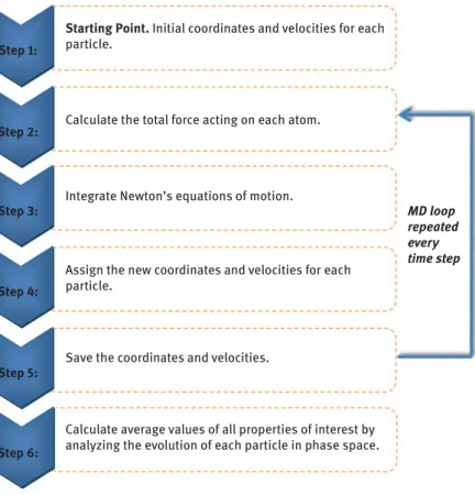
∂rⁱ , i=1,2, ...,N (5:4) whereidenotes any atom in the system,m_iits mass,riits position vector,Fithe force acting on it, andtthe time. Solving the 3N(whereNstands for the total number of atomistic units) second-order differential equations (eq. (5.4)), we track the time evolution of the system and obtain its trajectory, that is, the positions and velocities of all its atomistic units in time. Applying then basic principles of statistical mechanics [100], we can obtain estimates of several properties of interest (e.g., thermodynamic, structural, conformational and dynamic), which can be directly compared to experimental data. Figure 5.3 provides the basic structure of a typical MD algorithm.

To solve the equations of motion, a numerical integrator must be employed, which should guarantee efficiency, stability and accuracy. To this, the algorithm must:

– not require an expensively large number of force evaluations per time step (thus, very popular techniques for the solution of ordinary differential equations such as the fourth-order Runge–Kutta method become inappropriate);

– permit the use of a large time step;

– be fast;

– require little memory;

– satisfy the energy conservation law.

Over the years, several algorithms have been proposed that satisfy the above criteria.

The most popular are the gear predictor-corrector methods [92], the Verlet algorithms [93, 101] and the multiple time step methods (such as thereversibleREferenceSystem PropagatorAlgorithm or rRESPA [102]). In addition, thanks to the rapid growth of computing power, the development of robust parallelization techniques (based on domain [103–105] and force [106–107] decomposition and CUDA programming) and the availability of supercomputing infrastructures (computer machines with millions of CPU processors), highly complicated systems containing hundreds of thousands or even millions of interacting particles (corresponding to simulation boxes with edge

(18)

lengths equal to hundreds of nanometers) can be simulated today in full atomistic detail for times up to several microseconds. Also, highly parallelized, user-friendly MD simulation packages are commercially available or freely distributed; we mention:

– Large-scaleAtomic/MolecularMassivelyParallelSimulator,LAMMPS[107]

– GROningenMAchine forChemicalSimulations,GROMACS[108]

– AssistedModelBuilding withEnergyRefinement,AMBER – NAnoscaleMolecularDynamics,NAMD[109]

– Chemistry atHArvardMacromolecularMechanics,CHARMM

5.3 Atomistic MD simulation of graphene-based PMMA nanocomposites

As a model polymer, we have chosen PMMA whose nanocomposites with GS have been studied in detail over the years with several techniques. For example,

Calculate average values of all properties of interest by analyzing the evolution of each particle in phase space.

Save the coordinates and velocities.

Assign the new coordinates and velocities for each particle.

Integrate Newton’s equations of motion.

Calculate the total force acting on each atom.

MD loop repeated every time step Step 1:

Step 2:

Step 3:

Step 4:

Step 5:

Step 6:

Starting Point. Initial coordinates and velocities for each particle.

Figure 5.3:Simplified flow diagram of a typical MD algorithm.

(19)

Ramanathan et al. [39] used sonication to break rigid nanoplatelets of expanded graphite apart into thinner platelets, which were dispersed next in a PMMA solution using high-speed shearing methods. This led to an increase in theT_gby 29 °C at 0.05 wt.% loading of the matrix in FGS, and up to an 80% enhancement of the Young’s modulus at 1 wt.% loading in FGS. Similar observations have been reported by Li and McKenna [45] for GO/PMMA nanocomposites. One reason for the extraordinary mechanical properties of FGS-PMMA nanocomposites is the enhanced interfacial interactions of oxygen functionalities across the surface of graphene with PMMA chains. FGS contain pendant hydroxyl groups, which may form hydrogen bonds with the carbonyl groups of PMMA. Additional enhancement comes from the nanoscale surface roughness of FGS, the defects caused during thermal exfoliation of the precursor graphite oxide and their wrinkled topology at the nanoscale due to their extremely small thickness. These can enhance mechanical interlocking with the polymer chains, which also leads to better adhesion.

Atomistic MD simulations [62–63] have shown strong adhesion of PMMA chains (especially of its side groups) on graphene and considerably slower segmental and chain mobility in the interfacial area. According to simulation data, local mass density, segmental dynamics and chain terminal relaxation differ from the bulk behavior up to several nanometers from the graphene surface.

In the remaining of this chapter, we will focus on a methodology [110], initially proposed for a simpler class of systems (glassy vinyl polymers such as polypropylene and polystyrene) [110], which allows the determination of the mechanical properties of PMMA nanocomposites filled with GS (functionalized or nonfunctionalized), based on small-strain deformation experiments on the computer of microscopically detailed model structures. The procedure involves several modeling and mathematical steps and allows computing the elastic constants (Young’s modulus E, bulk modulus B, shear modulusGand Poisson’s ratioν) of a polymeric glass under the assumption that vibrational contributions of the hard degrees of freedom are not significant; as a result, estimates of the elastic constants can be obtained by computing changes only in the total potential energy of static microscopic structures subjected to simple deformation modes. For glassy atactic polypropylene for which the method was first developed and implemented by Theodorou and Suter [110], elastic constants were predicted within 15% of the experimentally measured values.

All the simulations have been performed with an all-atom force field, allowing for a direct comparison of the computed with available experimental data. We chose DREIDING [95] because it combines simplicity with accuracy (for acrylic polymers). Since DREIDING [95] does not provide information about the values of partial charges of PMMA atoms, these were borrowed by the OPLS-AA [96] force field.

Additional technical details (such as the parameter values of all bonded and nonbonded interactions describing intra- and interatomic contributions to potential energy) can be found in two published articles [72, 91]. Figure 5.4a–d provides typical

(20)

atomistic structures of a PMMA chain, a GS, a GO and a functionalized PMMA chain with pyrene groups added to its two ends.

Systems simulated and simulation strategy

We focus on sPMMA, atP = 1 atm. The simulations were performed with strictly monodisperse samples with the model system consisting of 27 chains of degree of polymerization X = 15 (corresponding to a molecular weight of 1,503.75 g/mol).

Unfunctionalized and functionalized GS had lateral dimensions 12 Å × 12 Å. Three model systems were studied: (a) the neat sPMMA matrix (no GS added; it will be denoted as sPMMA in the following), (b) its nanocomposite with three unfunctionalized monolayer GS (it will be denoted as GS-sPMMA in the following) corresponding to 5.67 wt.% concentration in GS and (c) its nanocomposite with three functionalized monolayer GS or GO (it will be denoted as FGS-sPMMA in the following) corresponding to 6.54 wt.% concentration in GO. The surface concentration of GO in hydroxyl (-OH) and epoxy (-O-) groups in the latter system was chosen to match as closely as possible the experimentally determined concentration reported by Ramanathan et al.

[39] through elemental analysis.

(a) (b)

(d) (c)

Figure 5.4:Typical atomistic structures of (a) an sPMMA chain, (b) a nonfunctionalized graphene sheet (GS), (c) a functionalized graphene sheet (FGS) and (d) a functionalized (py-sPMMA-py) chain.

(21)

To build initial configurations of all systems we used MAPS [111] and to execute the MD simulations we used LAMMPS [107]. All initial configurations were subjected to static structure optimization using a molecular mechanics algorithm to remove overlaps, and the resulting minimum potential energy structures were annealed to 500 K for several hundreds of nanoseconds to render them completely amorphous prior to quenching them down to room temperature, also to completely equilibrate them at all length scales. We used rectangular parallelepiped simulation cells of initial sides 40 Å × 40 Å × 40 Å subject to full periodic boundary conditions. Technical details regarding the execution of the MD simulations (type of thermostat–barostat used, calculation of electrostatic interactions, calculation of LJ interactions and of the tail corrections, integration of equations of motion, time step, etc.) can be found in the two relevant publications [72, 91].

Structural and conformational properties

From the equilibration runs atT= 500 K, we calculated several properties that provided a good picture of the effect of GS and GO on the structural, conformational and thermodynamic properties of the polymer matrix. Figure 5.5 shows a typical atomistic

Figure 5.5:Typical atomistic snapshot from the simulation with the FGS-sPMMA nanocomposite at 6.54 wt.% loading. The simulation cell contains 27 PMMA chains and three FGS with five hydroxyl groups and three oxygen atoms on their surface. Initial cell dimensions 40 Å × 40 Å × 40 Å. Carbon (sPMMA), carbon (FGS) and oxygen atoms are represented with gray, yellow and red colors, respectively. Hydrogen atoms have been omitted for clarity.

(22)

configuration of the FGS-sPMMA nanocomposite at the end of the MD simulation with this system atT= 500 K. A first quantity that can be easily calculated from an MD simulation in theNPTensemble is the densityρ. Our predictions areρ= 1.065 g/cm³ for the sPMMA,ρ= 1.082 g/cm³for the GS-sPMMA andρ= 1.091 g/cm³for the FGS- sPMMA system. The experimentally determined value for infinite molecular weight PMMA at the same temperature (500 K) is 1.072 g/cm³[112].

We also calculated (see Figure 5.6) the variation of polymer mass density with distance from a GS.

The high-density values (up to ~30% compared to the bulk density value) observed at distances up to ~5 Å from the surface of the GS indicate that sPMMA chains adsorb strongly on GS (either unfunctionalized GS or GO sheets). An example of a typical conformation of an adsorbed sPMMA chain on a GO is displayed in Figure 5.7.

An interesting point is that the local mass density of sPMMA is enhanced less in the FGS-sPMMA system than in the GS-sPMMA system. This should be attributed to the relative roughness of GO sheets (compared to the perfectly smooth surfaces of pristine GS) because of the presence of the characteristic -O- and -OH groups, which leads to the adsorption of less sPMMA molecules on GO than on GS. However, as we will see below, the -OH groups present on the surface of GO help the system develop a non-negligible number of hydrogen bonds with the oxygen atoms of sPMMA ester branches; this will be shown to have a strong impact on the overall mechanical performance of the nanocomposite. Figure 5.8 shows an example of a GO NP, which has developed two hydrogen bonds with one sPMMA chain on its one side and one hydrogen bond with another chain on its other side. The hydrogen bonds are highlighted with dashed circles in the figure. We clarify that the formation

1.6

(a) (b)

1.4 1.2 1.0 0.8 0.6 0.4 0.2 0.0

–20 –15 –10 –5 0

Distance from graphene sheet (Å)

𝜌 (g/cm3) 𝜌 (g/cm3)

5 10 15 20

1.6 1.4 1.2 1.0 0.8 0.6 0.4 0.2 0.0

–20 –15 –10 –5 0

Distance from graphene sheet (Å)

5 10 15 20

Figure 5.6:Local mass density normal to graphene sheets as obtained from the present MD simulations (T= 500 K,P= 1 atm) for the cases of pristine graphene sheets (a) and graphene oxide (b). The blue dashed line at the zero value of the horizontal axis denotes the average position of the graphene sheet midplane.

(23)

of hydrogen bonds is not imposed directly in our simulations, but it is the indirect result of the employed force field (particularly of the partial charges assigned to the various atoms).

Mechanical properties

For the estimation of the mechanical properties of the simulated systems, we followed the methodology first proposed by Theodorou and Suter [110] for an amorphous glassy polymer, to which the reader is kindly referred for more details. The method involves the selection of several (about 15) completely equilibrated configurations of the system, which are then submitted to deformation experiments, from which one can calculate in a rigorous way the elastic properties of the sample. At the temperature and pressure conditions of interest here (T= 300 K andP= 1 atm), sPMMA and its GS- or GO-nanocomposites are in the glassy state, implying that one cannot directly use MD to sample well-equilibrated system configurations because the simulations will be nonergodic (the system will be trapped in configurations characterized by a local minimum in their potential energy). One way to overcome this is to equilibrate the system at a higher temperature (above the melting point), where equilibration is much easier to achieve, select a good number of relaxed configurations from this simulation and subject them to cooling runs down to the lower temperature (T= 300 K), followed by a short MD run for the density and local structure to equilibrate further. The resulting glassy structures will then be good candidates to use in the subsequent computational deformation experiments for the estimation of the elastic constants (Young’s, bulk, shear moduli and Poisson’s ratio). The results can be significantly improved by aver- aging over all configurations subjected to deformation.

Figure 5.7:Atomistic snapshot from the MD simulation atT= 500 K showing a typical sPMMA chain configuration next to a GO.

(24)

Applying the methodology [110] to the systems studied here, we obtained the results shown in Table 5.1. From the numerical data presented in Table 5.1, we can draw several conclusions:

1) The predicted values of the Young’s modulus, shear modulus, bulk modulus and Poisson’s ratio for the pure sPMMA system are in an excellent quantitative agreement with reported experimental values, which are summarized in ref. 72.

2) A significant enhancement of the mechanical properties of both types of nanocomposites (GS-PMMA and FGS-PMMA) is observed. This is more pronounced for the FGS-based ones, which should be attributed to the development of hydrogen bonds between the filler (GO) and the polar chains (sPMMA).

(a)

(b)

Figure 5.8:An example of a situation where three hydrogen bonds develop between a GO and the surrounding sPMMA chains. We can observe the formation of two hydrogen bonds with the same chain on the one side of the GO (a) and of one hydrogen bond with a different chain on the other side of the GO (b).

(25)

To further appreciate the effect of graphene and GO on the mechanical reinforcement of PMMA, we have normalized the predicted values of the four elastic constants with the values corresponding to the pure sPMMA matrix, and the results are shown in Figure 5.9.

Overall, our results are in a good qualitative agreement with the experimental work of Ramanathan and coworkers [39] who reported an increase in the Young’s modulus of

~80% in PMMA samples modified with FGS. However, a direct comparison of our simulation results with the experimental data is difficult to make because the molecular weight of the polymer matrix and the size of graphene flakes used in the experimental measurements are too large to address with atomistic MD simulations.

Table 5.1:Predicted elastic constants for all simulated systems from our study.

System Lamé constants Elastic constants

μ(GPa) λ(GPa) E(GPa) B(GPa) G(GPa) ν

Pure sPMMA . . . . . .

Experimental values – – .–. .–. .–. .–.

GS-sPMMA . . . . . .

FGS-sPMMA . . . . . .

1.0

Young’s modulus Bulk modulus Shear modulus sPMMA GS-sPMMA FGS-sPMMA

1.2 1.4 1.6

Normalized values

1.8 2.0 2.2

Figure 5.9:Summary of property improvement for the elastic constants of GS-sPMMA and FGS- sPMMA nanocomposites (T= 300 K,P= 1 atm). Numerical values have been normalized with the corresponding value of the neat PMMA matrix at the same conditions (E= 3.4 GPa,B= 4.2 GPa, G= 1.3 GPa andν= 0.36).

(26)

Graphene agglomeration in the PMMA matrix and how to prevent it

The homogeneous dispersion of GS in a polymer matrix is perhaps the most important and challenging issue in the fabrication of graphene-based polymer nanocomposites.

In principle, GS fine dispersion offers larger areas for the effective adsorption of polymer chains, thus also for the better improvement of the properties of the nanocomposites.

All calculations reported in the previous section were carried out with model systems characterized by a uniform distribution of GS in the polymer matrix.

However, several times during the MD equilibrations atT= 500 K, GS agglomeration was observed to occur at long times, as GS exhibited a strong tendency to come close to each other and form graphitic (π–πstacking) structures. To gain a better understanding of such a phenomenon, we conducted an additional simulation study with a larger system containing 100 atactic PMMA (aPMMA) chains with degree of polymerizationX= 30 and six GS of size 60 Å × 60 Å (system 1), and we monitored the time evolution of the positions of the six GS inside the simulation box. The results are shown in Figure 5.10a, where aPMMA chains have been omitted for clarity. We see that already from the first two nanoseconds of the simulation, a pair of GS have come close to each other to form an agglomerate.

To overcome the problem of GS agglomeration, we proposed [91] a novel methodology, which relies on the functionalization not of GS but of a good fraction of PMMA matrix chains by adding pyrene groups to their ends. The functionalized chains are noted as py-PMMA-py (see Figure 5.4d). The key idea is that pyrene groups adsorb strongly on the surface of GS due to very favorableπ–πinteractions developing between their four benzene rings and the corresponding hexagonal structures of GS;

then, the intervening polymer mass between the two GS prevents them from ap- proaching one or the other, thus self-assembly is avoided. To test the idea, we repeated the simulation of system 1 at the same temperature and pressure conditions (T= 500 K andP= 1 atm) by replacing approximately 40% of the aPMMA chains in the matrix with functionalized py-PMMA-py chains (system 2). The time evolution of the positions of GS for such a system is shown in Figure 5.10b. To enable a one-to- one comparison between the two systems (system 1 and system 2), the initial positions and initial velocities of all atoms in GS in the simulation with system 2 matched exactly those in the simulation with system 1. Then, according to Figure 5.10b, for the entire duration of the simulation (~500 ns), the six GS remained homogeneously dispersed in the polymer matrix. It is also clear that many of the pyrene groups of the functionalized py-PMMA-py chains were adsorbed strongly on the surface of GS.

To shed additional light in our MD findings, we calculated the time evolution of the distances between the centers of mass of all GS pairs in the two simulated systems. The results are shown in Figure 5.11a and b for system 1 and system 2, respectively. For system 1, we see that the distances between GS in pairs 1–4, 2–3 and 5–6 suddenly dropped down to 3.4 Å att= 3, 10 and 120 ns, respectively, which is the

(27)

characteristic distance between consecutive graphene planes in a typical graphitic structure, and remained to 3.4 Å throughout the simulation. In contrast, for system 2, no such phenomenon was observed. The reason for this behavior is the strong adsorption of functionalized py-PMMA-py chains on the surface of GS by their end-pyrene groups. A characteristic example is depicted in Figure 5.12, showing a GS on the surface of which 10 pyrene groups from different py-PMMA-py chains have been adsorbed.

t = 0 ns (a)

(b)

t = 2 ns

t = 10 ns t = 150 ns

t = 0 ns

t = 500 ns

Figure 5.10:(a) Evolution of GS self-assembly during the MD simulation with the aPMMA-GS nanocomposite in the absence of py-PMMA-py chains. (b) Same as with (a) but for the case where 40% of aPMMA chains have been replaced by functionalized py-PMMA-py chains.