2. Properties of Graphene Materials

(1)

Application of graphene in electrochemical sensing

Dissertation

Zur Erlangung des Doktorgrades der Naturwissenschaften (Dr. rer. nat.)

der Fakultät für Physik der Universität Regensburg

vorgelegt von Masoumeh Sisakhti

aus Shiraz, Iran

im Jahr 2016

(2)

Das Promotionsgesuch wurde am 25.10.2016 eingereicht.

Das Kolloquium fand statt am 09.12.2016

Prüfungsausschuss: Vorsitzender: Prof. Dr. Gunnar S. Bali 1. Gutachter: Prof. Dr. Christoph Strunk 2. Gutachterin: Prof. Dr. Antje J. Bäumner weiterer Prüfer: Prof. Dr. Rupert Huber

(3)

To my best friend, Ali

(4)

List of Publications

This thesis is based on the following publications:

1) Signal enhancement in amperometric peroxide detection by using graphene materials with low number of defects

A. Zöpfl, M. Sisakthi, J. Eroms F.M. Matysik, C. Strunk and T. Hirsch (Microchim. Acta, 183, (2016) 83–90)

2) Perforated graphene/NiO nanoparticle composites for high performance electrochemical sensors

M. Sisakhti et. al, (to be submitted)

(5)

Abstract

Graphene possesses distinctive properties such as chemical stability, wide potential window and large surface area, making it an ideal electrode material that could potentially yield significant benefits in many electrochemical applications. The quality of graphene has an enormous impact on its electrochemical performance. It is therefore necessary to study the influence of defects and impurities on the amperometric performance of graphene towards the sensing of a target analyte. This thesis studies the critical role of the fabrication routes of graphene materials on their efficiency and electrochemical performance, putting emphasis on the influence of defects and impurities on direct amperometric detection of hydrogen peroxide. It is found that the sensors based on graphene with lower number of defects lead to a higher sensitivity towards H₂O₂.

Furthermore, graphene's electrochemical and amperometric properties for non-enzymatic glucose determination based on electrodeposition of NiO nanoparticles have been investigated. To address this issue, CVD graphene was patterned with arrays of antidot lattices to provide artificial dangling positions for attachment of nanoparticles to the graphene surface. It is demonstrated that the nanopatterned graphene exhibited better performance in glucose sensing compared to pristine CVD graphene, and efficient tailoring of the size and lattice constant of the antidots on graphene surface can optimize electrodeposition of NiO nanoparticles and the amperometric response of graphene-based sensors towards glucose detection.

(6)

List of Figures

Figure 1.1. Graphene, a 2D building material for carbon materials of all dimensionalities ... 2

Figure 2.1. Lattice structure of graphene ... 6

Figure 2.2. Band structure plot for graphene. Image from [Li10]. ... 7

Figure 2.3. Energy dispersion as a function of the wave-vector components ... 8

Figure 2.4. Energy gap in a conventional semiconductor vs graphene: ... 9

Figure 3.1. Biosensor components ... 14

Figure 3.2. List of key characters of a biosensor ... 15

Figure 3.3. Summary of enzymatic glucose oxidation mechanisms ... 18

Figure 4.1. Basic diagram of a potentiostat and a three-electrode cell ... 23

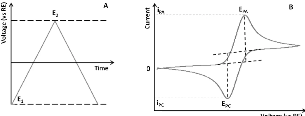
Figure 4.2. Principles for the generation of a CV curve. ... 24

Figure 4.3. Simple Randles equivalent circuit for an electrochemical cell ... 27

Figure 5.1. Micromechanical exfoliation of graphene. ... 31

Figure 5.2. Proposed structure of graphite oxide (GO) based on the Lerf–Klinowski model . 32 Figure 5.3. rGO deposited microelectrodes ... 33

Figure 5.4. Two-step photolithography for preparation of the CVD graphene electrodes ... 35

Figure 5.5. Typical Raman spectra for a single-layer graphene and bulk graphite ... 36

Figure 5.6. Raman spectra of graphene produced via different routes... 37

Figure 5.7. CV performed to prove the successful shielding of the gold contacts. ... 38

Figure 5.8. Chronocoulometric measurements for different electrodes ... 39

Figure 5.9. EIS spectroscopy for graphite, rGO, CVDG and SG ... 40

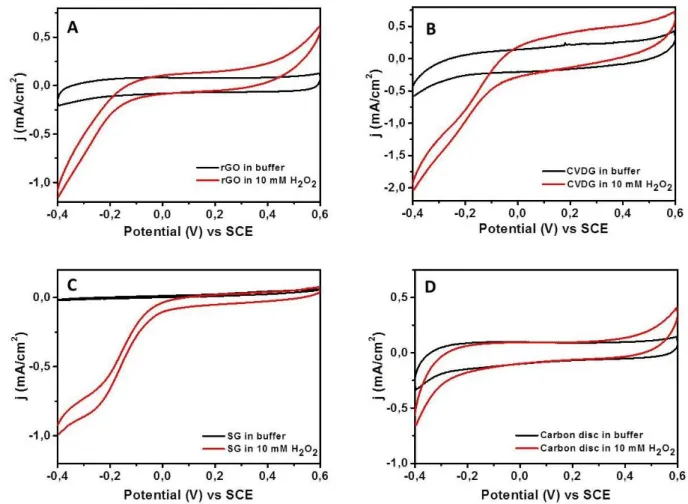
Figure 5.10. Steady state current density/voltage cycles for different electrodes ... 42

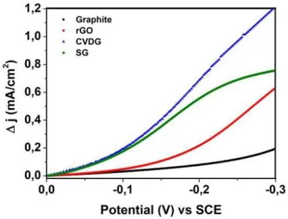
Figure 5.11. Change in current density for H2O2 reduction during the cyclic voltammetry .... 43

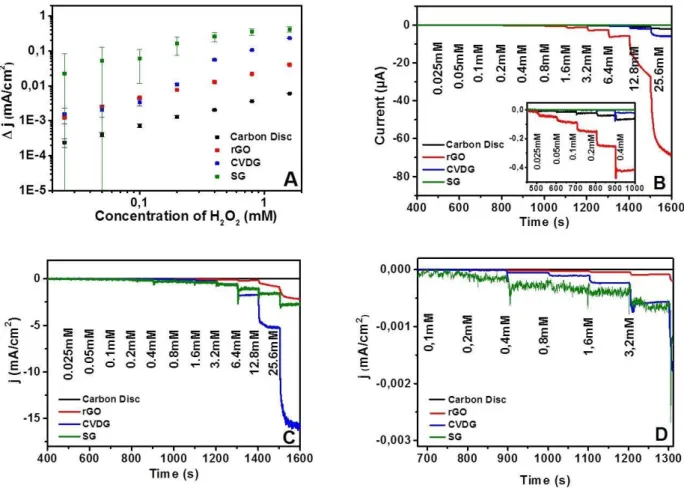
Figure 5.12. Electrochemical behavior of electrodes to growing concentration of H2O2 ... 44

Figure 5.13. The magnified view of the current density/[H₂O₂] ... 45

Figure 6.1. Schematics of EBL and RIE processes for creation of antidot lattices ... 50

Figure 6.2. SEM image of the CVDG on Si/SiO2 substrate structured with antidot lattices ... 51

Figure 6.3. Raman spectra recorded on CVDG modified by antidots of 70nm diameter with different lattice constants ... 51

Figure 6.4. SEM image of electrodeposited NiO nanoparticles on graphene ... 54

Figure 6.5. Electrochemical behavior of NiO/graphene electrodes toward glucose. ... 54

Figure 6.6. SEM images of the electrodeposited NiO nanoparticles on graphene modified with antidots of the same hole diameter (70nm) and different lattice constants ... 56

Figure 6.7. SEM images of the electrodeposited NiO nanoparticles on graphene modified with antidots of the same lattice constant (500nm) and different hole diameters ... 57

Figure 6.8. Density of electrodeposited NPs on graphene vs lattice constant and diameter .... 57

Figure 6.9. CV of the NiO/ antidot-modified-graphene electrodes in the absence and presence of glucose ... 58

Figure 6.10. Electrochemical behavior of electrodes with different lattice constants toward growing concentration of glucose ... 59

Figure 6.11. Study of response reproducibility and stability ... 60

Figure 6.12. Investigation of the sensor’s selectivity ... 61

(9)

Figure 8.1. Schematic immobilization of GOD into GO sheets via peptide bonds ... 69

Figure 8.2. Sensing performance of GOD immobilized EDC/NHS/graphene to glucose. ... 69

Figure 8.3. Sensing performance of GOD immobilized Nafion/graphene to glucose. ... 71

Figure 8.4. Schematic illustration of grafting a diazonium salt to a graphene sheet... 71

Figure 8.5. Changes in the Raman spectrum of graphene due to NBD-functionalization. ... 72

Figure 8.6. Sensing performance of GOD immobilized Nafion/graphene to glucose. ... 73

(10)

1

When nature finishes to produce its own species, man begins using natural things in harmony with this very nature to create an infinity of

species.

the artist-scientist Leonardo da Vinci

1. Introduction

The key role of carbon atoms in all living organisms is unquestionable. However, for a long time only two main variants of carbon were known: diamond and graphite, both crystalline forms of the carbon element. Diamond possesses a covalent structure, with each carbon covalently bonded to four other carbon atoms in a tetrahedral arrangement to form a rigid, transparent, and insulating structure with a band gap of about 6eV. Unlike diamond, graphite is a soft and conducting structure, in which each carbon covalently bonds to three other carbon atoms in a hexagonal arrangement.

The first use of graphite can be traced back to the 4th millennium B.C. when Boian culture applied it as a ceramic paint to decorate pottery in southeastern Europe [Boa 82]. It consists of many sp² hybridized one-atom-thick sheets of carbon lattice stacked on top of each other, coupled via weak Van Der Waals forces. The band theory of graphite has been studied from 1947, when P. R. Wallace used the tight binding approximation method, which assumes conduction only happens in one layer which is graphene layer [Wal47]. Graphene, a two- dimensional (2D) monolayer of carbon atoms tightly packed into a honeycomb lattice, is basic building block for graphite and other graphitic materials of all dimensions (Figure 1.1) [Gei07].

Initially, it was believed for many years [All09] [Pei35] [Mer68] that strictly 2D crystals were thermodynamically unstable and could not exist. The experimental observations witnessed thata divergent contribution of thermal fluctuations in low-dimensional crystal lattices should lead to such displacements of atoms that they become comparable to interatomic distances at any finite temperature. For that reason, existence of such one-atom-thick graphene could not be reconciled with theory and graphene was just used for theoretical analysis until 2004, when Novoselov et al [Nov04] demonstrated the possibility to isolate it in a simple way. Since then many groups have undertaken the task of investigating graphene’s electronic, mechanical and thermal properties both experimentally and theoretically [Cas09] [Sca09] [Bal08] [Bun08].

Graphene possesses many properties that make it an interesting candidate for researches and applications in various areas. Ballistic transport of electrons along the atomically thin layer, together with mobilities exceeding 300000 cm²V^-1S^-1 and an ambipolar field effect make graphene an ideal material for the next generation of semiconductor devices [All09][Guo12].

Although the lack of a bandgap limits the usage of two dimensional graphene for digital

(11)

2 switching, where high on/off ratios are necessary, the possibility of opening bandgaps lithographically by fabricating graphene nanoribbons enables graphene to be regarded as a possible candidate for electronic devices in the future [Mer08].

Beside these promising properties, other extraordinary features of graphene are also discussed. For instance the large and planar surface area of a single sheet and low electrical noise of graphene field effect transistors make it possible to be considered in optoelectronic and sensor applications [Bao12] [Bon10] [Koc13].

Figure ‎1.1. Graphene, a 2D building material for carbon materials of all dimensionalities. It can be wrapped up into 0D buckyballs, rolled into 1D nanotubes or stacked into 3D graphite. Image from [Gei07].

One area of particular interest where graphene has emerged as a rapidly rising star is electrochemistry, which has widely benefited from the application of graphene as an electrode material within a variety of sensing and energy storage devices [Xio14] [Amb14]. An essential characteristic of an electrode material is its surface area, which is important in applications such as energy storage, biocatalytic devices, and sensors. Exhibiting a theoretical surface area of 2630 m² g⁻¹, graphene materials have been considered to hold great promise for many applications, in particular as electrode material, claiming superior electrochemical performances when compared to traditional noble metals and various carbon based electrode materials, such as graphite and carbon nanotubes (CNTs) [Pum09] [Bro10].

Clearly, there are a variety of graphene materials with different properties. Some examples include mechanically exfoliated pristine graphene [Nov04], reduced graphene oxide [Eda08], chemical vapor deposited graphene [Kat14] and epitaxial graphene [Rie10]. The tremendous progress in the fabrication of graphene has provided the possibility to use them in a controllable and reproducible fashion in scientiﬁc experiments. Essential is the ability to fabricate individual single layer graphene sheets. This can be achieved by different means, for instance, micromechanical cleavage of graphite through which graphene sheets are directly deposited onto the substrate by mechanical cleavage. This approach, also known as the

(12)

“scotch-tape” method [Nov04], is widely used in many laboratories to obtain pristine perfect- structured graphene, but is restricted to small sample dimensions with incontrollable shape, size and location.

Chemical reduction of graphite oxide, usually based on Hummers method [Hum58] is considered to be the most economical way to produce reduced graphene oxide, with some advantages such as scalable, high volume production and ease of chemical modification.

However, this approach does introduce some defects in graphene during the oxidation or reduction steps, and results in abundant structural damage of the graphene.

A more controllable process for synthesis of graphene is chemical vapor deposition (CVD).

Recent development in the CVD process has led to the preparation of wafer-scale graphene ﬁlm on metal substrates (Ru [Sut08] [Log09], Ni [Kim09] and [Rei09] and Cu [Hu12]) with single-layer yield as high as 95%. Although the CVD-graphene can only be produced on certain metallic substrates and it requires additional transfer steps, leading to some contaminations and destruction of graphene sheets, it still provides high conductivity and transparency, which allows electronic and electrochemical sensors to beneﬁt from the high- yield and high-quality CVD graphene and enables the mass production of devices with high reproducibility.

The significance of knowing what sort of graphene with what properties we are utilizing, especially becomes noticeable when it comes to the fundamental issue of the electrochemical performance of graphene, where the role of defects and impurities can be considerable towards the sensing of a target analyte [Kum13] [Lin11]. In particular, as we learn from the plethora of different properties attributed to the graphene, the presence and role of such defects and impurities must be recognized and characterized. Raman spectroscopy, as will be discussed in section 5.2, can be used to determine the number of graphene layers and stacking order as well as density of defects and impurities. The critical role of the characterization of graphene materials fabricated by different methods is particularly important for a comparison between the efficiency and electrochemical performance of different graphene materials.

However, regardless of the preparation methods, graphene-based electrodes have demonstrated their utility in electrochemical sensors for detection of different biomolecules, as addressed in plenty of works [Pum11] [Wan11]. Extensively, biosensors based on enzymes have been researched [Sha10], where enzyme immobilization of modified graphene has been employed in order to construct efficient biosensors, suitable for selective and rapid analysis of various biological species in vivo and in vitro. However, the performance of enzyme-based sensors is greatly limited by enzyme immobilization techniques and detection environments (pH, temperature, etc.). In addition, natural enzymes are both expensive and unstable due to the intrinsic nature of the enzymes. Therefore, enzyme-free sensing is highly desirable and has the advantage of high stability, simplicity, good reproducibility, and low cost.

The present work aims at application of graphene for electrochemical sensing, investigating methods for graphene modification and functionalization, in order to improve the sensitivity and stability of the electrochemical sensors based on graphene.

(13)

4 This dissertation is divided into eight chapters, following the line of concepts indicated in the introduction section. In chapter 2we will provide a thorough introduction to the electronic properties of graphene materials, employing tight binding argumentation and then briefly review those aspects of graphene’s properties most relevant to electrochemical applications.

Chapter 3 delivers an overview of the general concept of electrochemical sensors, following an introduction to enzymatic and nonenzymatic approaches for electrochemical detection of glucose.

In chapter 4 an introduction is given on the electrochemical instrumentation and detection techniques utilized in this project, which is beneficial for understanding and interpretation of the performed experiments and achieved results.

Chapter 5 begins with an overview of the sample preparation steps of different graphene materials and focuses on the influence of the structural defects and device fabrication routs on the signal enhancement in non-enzymatic detection of hydrogen peroxide.

The main results of our efforts for fabrication of a graphene-based electrochemical glucose sensor will be presented in chapter 6, which mainly deals with the introduction of antidot lattices on graphene surface and their role on non-enzymatic sensing of glucose.

At the end of this work, chapter 7 summarizes the main findings of this thesis, presenting a brief outlook onto possible future experiments to employ graphene as an electrode material for fabricating an array biosensor and thereby detecting numerous target analytes simultaneously. This chapter is followed by an appendix (chapter 8), which mainly deals with the many additional experimental techniques used throughout this work to functionalize graphene surface through introduction of variable decorations both covalently and noncovalently. This chapter is particularly beneficial for those readers who are interested in studying enzymatic detection of glucose based on CVD graphene.

(14)

5

2. Properties of Graphene Materials

This chapter summarizes the most important structural and electrochemical characteristics of graphene materials. In the ﬁrst part of this chapter we introduce the band structure of graphene and explain how the band structure calculated through tight binding model will cause the charge carriers in graphene to be viewed as massless Dirac fermions.

The remainder of this chapter is dedicated to electrochemistry of graphene and sensing and biosensing applications of graphene, which will be the focus of the next chapters of the work.

2.1 Structural properties of graphene

The carbon atoms in a graphene layer are sp²-hybridized (one s-orbital and two p-orbitals hybridize together), forming three in-plane σ-bonds per atom which in turn leads to the formation of a hexagonal planar layer with a honeycomb-like atomic arrangement. The hexagonal graphene lattice is displayed in a top view model in Figure 2.1 (A) and exhibits a basis with two carbon atoms, A and B, per unit cell. These two atoms make up two non- equivalent sublattices in graphene, with an interatomic nearest neighbor separation of a= 1.42 Å. The A atoms are connected only to B atoms and vice versa, this is called a bipartite lattice.

The real space unit vectors of the hexagonal lattice forming the basis of the unit cell are expressed as: and [Cas09], while the corresponding reciprocal lattice vectors , can be written as:

and , defined by the condition , i.e. the direction of the unit vectors and of the reciprocal lattice are related by 90° from the unit vectors and of the hexagonal lattice in real space. The three nearest-neighbor vectors in real space are given by , , .We define the first Brillouian zone (FBZ) of the reciprocal lattice in the standard way, as bounded by the planes bisecting the vectors to the nearest reciprocal lattice points, illustrated in Figure 2.1 (B). This gives an FBZ of the same form as the original hexagons of the honeycomb lattice, but rotated with respect to them by / 2.

(15)

6

Figure ‎2.1. Lattice structure of graphene (A) The honeycomb lattice structure of graphene showing the unit cell in real space, which contains two sublattices marked A and B. The 2D-real space unit vectors and are also indicated. (B) the first Brillouin zone of graphene with the reciprocal unit vectors, _and , and high symmetry points Γ, M, K and K′.

Of particular importance for the physics of graphene are the three high symmetry points Γ, K and M at the center, corner and center of the edge in the BZ respectively. In graphene, most of the interesting physics occur near the two inequivalent BZ corners K and K′, where the bands cross the Fermi energyE_F. These are named Dirac points and their positions in momentum space are given by and . If we change the role of and lattice points we actually reverse our time (flipping a vector gives a vector). The time reversal is also connected to the chirality of particles: reversing time changes the roles of particles and antiparticles (electron and holes in our case). So the and states are not equivalent (e.g. an electronic state in forces the state to be positronic).

The electronic band structure of graphene shows a very interesting conic point at the and points in the Brillouin zone. The linear bands cross exactly at the Fermi energy, so that there is only one state, which can be treated as a hole or as an electron. Since there are no conducting states at the Fermi level, graphene behaves like a gapless semiconductor (also called semi-metal).

2.2 Electronic Structure of graphene in the tight binding model

As mentioned before, each non-equivalent carbon atom in the unit cell has four valence electrons, three out of which form strong σ covalent bonds at high binding energy, giving graphene exceptional mechanical strength and structural rigidity within its layers.

The σ bonding sp² orbitals are formed by the superposition of the s, px and py orbitals of atomic carbon leaving the pz orbital unhybridized. The pz-orbitals of neighboring carbon atoms overlap and form the distributed π-bonds that reside above and below each sheet and cross the Fermi energyE_Fat the BZ corners K and K′ (Figure 2.2). These delocalized π orbitals are responsible for the excellent conductivity in graphene and all the intriguing physics.

(16)

Figure ‎2.2. Band structure plot for graphene. Image from [Li10].

One of the simplest evaluations of the band structure and therefore the electronic properties of graphene can be derived from the tight binding approximation for the band theory of graphite, which was developed by Wallace long before graphene existed [Wal47]. This model is valid when the overlap of the wave function is large enough so that corrections to the isolated atoms are needed while at the same time not too large to invalidate the atomic description. In this case, the wave function for electrons can be approximated by a linear combination of the atomic wave functions. Thus the tight binding model is also known as the linear combination of atomic orbitals (LCAO) approximation.

In the atomic description, the Hamiltonian for each carbon atom localized at and is [Zho07]:

(2.1) where V_ais the atomic potential on each carbon atom.

The atomic wave function centered on each carbon site satisfy

(2.2) In graphene, the total Hamiltonian is:

. (2.3) The total Hamiltonian can be rewritten as the Hamiltonian for atom 1 or 2 with some corrections (H₁andH₂) which take care of the potential created by all other atoms.

(2.4)

The Bloch wave function is

(2.5) where the wave function ϕ is a linear combination of the localized wave functions

(2.6) Here and are constants and

The eigenenergies can be obtained by solving the Schrödinger equation

(2.7)

(17)

8 yielding to

)

(2.8) Here is a small correction to the overall energy, defined as , the next nearest neighbor hoping integral defined as , and . Figure 2.3 shows the π band dispersion of graphene. The valence and conduction bands touch only at the six corners of the BZ. Since each carbon atom contributes one electron, the valence band is completely filled up to the Fermi level, where the valence and conduction bands merge. Because of this, graphene is known as a semi-metal or zero-gap semiconductor.

Figure ‎2.3. Energy dispersion as a function of the wave-vector components k_x and k_y. The lower and the upper surfaces denote the valence and the conduction energy bands, respectively. Image from [Cas09].

2.2.1 Massless Dirac fermions and massive quasiparticles

The low energy electronic structure of graphene near the corners of the BZ is extremely important since it determines the transport properties as well as various exotic phenomena observed in graphene.

To obtain the low energy electronic structure near the zone corners K (K′), we expand to the first order around the Brillouin zone corners K, :

(2.9) Eq. 2.16 reduces to

. (2.10) Thus the Hamiltonian is

(2.11) where and are the Pauli matrices and . The dispersion relation in Eq.

2.11 becomes . This is analogous to the dispersion relation formulated in Einstein’s relativistic theory , with zero effective mass

(18)

m=0 and the speed of light c replaced by the Fermi velocity,v_F, which is ≈300 times smaller.

This suggests that electrons in graphene are governed by a two-dimensional version of the relativistic quantum theory introduced by Dirac, which holds for massless relativistic Fermions (e.g. neutrinos). Because of this, the low energy quasiparticles in graphene are also described as “Dirac fermions” and the points where the valence and conduction bands merge are called “Dirac points”. This Dirac physics of the charge carriers is the root cause of a lot of interesting physics observed in graphene. Starting from the very first observation of an anomalous, so called half integer, quantum Hall effect in graphene [Nov07] [Zha05] where the sequence of steps in the Hall conductivity is shifted with1/ 2, with respect to the classical quantum Hall effect. Another consequence of the gapless linear bands is the peculiar scattering properties of the charge carriers, which for certain incidence angles on electrostatic potential barriers can have a transmission probability of 1 [Bee08]. This, so called Klein tunneling causes the charge carriers in graphene to be unhindered by electrostatic potentials [Rob12].

Perhaps the most interesting aspect of graphene physics is that the band structure and physical properties of this material may be influenced by nanostructuring, functionalizing, mechanically straining, etc., yielding rich new physics to be studied and exploited [Fuh10]

[Gei07] [Bar09].

Figure 2.4 shows a schematic drawing of the low energy dispersion nearE_F. The peculiar linear dispersion for the valence and conduction bands results in many intriguing properties.

First of all, the “Fermi surface” in graphene contains only six points, rather than a true Fermi surface. Because of the finite number of points at the Fermi surface, the density of states is vanishingly small atE_F.

Moreover, the linear dispersion also gives rise to many properties in graphene that are different from those in two dimensional semiconductors.

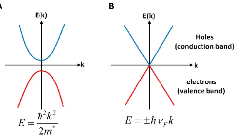
Figure ‎2.4. Energy gap in a conventional semiconductor vs graphene: Energy dispersion of (a) a typical two- dimensional semiconductor and (b) that of graphene, which is a zero-gap semiconductor.

(19)

10 In semiconductors, the typical band dispersions show a quadratic behavior (Figure 2.4), and the electrons can be described by nonrelativistic theory formulated in Schrödinger equation.

An electron in these systems is modeled as a quasi-particle with a finite (“massive” compared to zero) effective mass . The mass is usually different from the non- interacting electron mass and this mass renormalization is used to take into account the effects of electron-electron interaction and electron-phonon interaction. The velocity of electrons changes as a function of electron binding energy. The electron in graphene, however, shows a linear dispersion relation and travels with a constant velocity.

2.3 Basic electrochemistry of graphene

One area which has considerably benefited from carbon based materials is the field of electrochemistry, where carbon materials are at the forefront of innovation and widely utilized both analytically and industrially. As indicated in many studies, carbon materials have the potential to outperform the traditional noble metals in many areas [Bro11]. In particular, graphene has been reported to be advantageous in various electrochemical applications ranging from sensing through to energy storage and generation [Bro11] [Rac15]. This diversity and success stems largely from the often-cited advantages of graphene, including chemical stability, low cost, wide potential window, relatively inert electrochemistry, rich surface chemistry and electro-catalytic activity for a variety of redox reactions [Bro14]

[Mcc08].

It has been shown that graphene exhibits high electrochemical capacitance with excellent cycle performance and hence has potential application in ultracapacitors [Sto08] [Mis11].

Shao et al. reported that graphene shows much higher electrochemical capacitance and cycling durability than CNTs. The specific capacitance was found to be ∼165 and ∼86 F/g for rGO and CNTs, respectively [Sha10c].

The electrochemical properties of graphene as electrode materials have been highly explored recently. It is well established that the choice of electrode material has a significant effect on the observed electrochemical signature in terms of the electrode’s geometry, choice of composition and surface structure [Bro14]. When reviewing the essential characteristics of an electrode material for widespread applicability within electrochemistry, graphene’s advantages become apparent. Due to its favorable electron mobility and unique surface properties, such as one-atom thickness and high specific surface area, graphene can accommodate the active species and facilitate their electron transfer at electrode surfaces.

Furthermore, the high surface area of graphene facilitates large amounts of electroactive sites, which is favorable for loading high amount of biological species on the electrodes employed in electrochemical sensing applications.

Graphene’s conductivity remains stable over a vast range of temperature, encompassing stability at temperatures as low as liquid Helium, where such stability is essential for reliability within many electrochemical applications [Bro10].

(20)

Considering the arguments already mentioned, graphene holds inimitable properties that are superior in comparison to other carbon allotropes of various dimensions and from any other electrode material, thus suggesting that graphene is a more favorable electrode material that could potentially yield significant benefits in many electrochemical applications.

2.4 Graphene for sensing applications

The beneficial implementation of graphene as a sensor substrate has been widely reported for the detection of a diverse range of analytes including numerous bio-molecules, gases and miscellaneous organic and inorganic compounds.

Graphene-oriented sensors can be expected to be highly sensitive for detecting individual molecules on and oﬀ its surface. The high sensitivity of graphene emerges due to two primary reasons: 1) the 2D nature of graphene allows total exposure of all of its atoms to the adsorbed target molecule, providing the high surface area per unit volume, and 2) it is inherently a low- noise material due to the quality of its crystal lattice, which leads to screen charge fluctuations more than one dimensional systems such as CNTs [Ali16].

Furthermore, graphene is an excellent conductor of electrical charge. Heterogeneous electron transfer (the transfer of electrons between graphene and the molecule in the solution necessary for the oxidation/reduction of electroactive species) occurs at the edges of the graphene or at plane defects, rather than the basal plane-the latter is sometimes referred to as being inert-due to the oxygen-containing groups present at the graphene edges.

The realization of devices employing such properties has been tried in various graphene-based systems over the last few years. For instance, a graphene-based gas sensor has been demonstrated to be one of the promising materials allowing the ultimate sensitivity, detecting the adsorption of individual gas molecules with fast response time at room temperature [Sch07].

The working principle of graphene devices as gas sensors is based on the changes of their electrical conductivity induced by surface adsorbates, which act as either donors or acceptors associated with their chemical natures, preferential adsorption sites and the surrounding atmospheres [Sch07] [Col00] [Ao08]. By monitoring changes in resistivity, minute concentrations of certain gases present in the environment can be well sensed. Till now, a number of groups have demonstrated good sensitivity for the detection of NO₂, NH₃, and other gaseous molecules under ambient conditions by using chemically derived graphene- based sensors [Ao08] [Hua08] [Fow09]. Some reports have also confirmed high sensitivity of sensors based on graphene nanocomposites decorated with metals and metal oxides for hydrogen [Alm10] [Lan11], carbon monoxide [Say15] and ethanol [Jia11] in the gas phase.

Another enticing scope is the use of graphene in biological devices for biosensing, where the excellent electrochemical and structural properties of graphene open up possibilities for designing and preparing graphene-oriented electrodes for a wide range of biosensing applications. Although CNTs offer many advantages in fabricating electrochemical devices,

(21)

12 graphene with favorable properties compared to CNTs, has opened a new horizon in the field of electrochemical sensing and biosensing applications. The primary distinguishing characteristics of graphene in comparison to CNTs are graphene’s high biocompatibility, ease of processing, low cost and facile chemical functionalization, which offer a better alternative for high performance chemical and biological sensors [Vam06].

Additionally, graphene’s high surface area to volume ratio provides more uniform distribution of electrochemically active sites than electrodes made from graphite and CNTs [Pum09]. This is advantageous for higher enzyme loading, thereby increasing the sensitivity of graphene- based biosensors [All10], since the whole surface area can be activated and even small changes in the charge environment caused by the adsorption of molecules can give measurable changes in their electrical properties [Yan10].

Graphene-based materials are considered to provide a suitable microenvironment for biomolecules immobilization, facilitating electron transfer between the immobilized biomolecules and electrode substrates. Novel graphene-based biosensors have been made regarding the fact that graphene oxide possess reactive functional groups that can easily bind with the free –NH2 terminals of the enzyme or protein to result in a strong amide covalent linkage [Sha09] [Alw09] [Kan09].

Graphene materials have also been employed for sensitive and selective electrochemical detection of nucleobases, nucleotides, single stranded DNAs (ssDNA), and double stranded DNAs (dsDNA), where the existence of π-rich conjugation domains gives graphene the ability to interact with DNA molecules via π-π stacking interactions. Such electrochemical DNA sensors may provide a simple alternative approach for DNA analysis and sequencing [Liu12].

Stacked graphene nanofibers have been reported to be used to distinguish the four nucleobases, resulting in a sensitivity two to four folds higher than CNT-based electrodes, due to numerous open edges of individual graphene nanosheets which are much more electrochemically active compared to the basal carbon plane [Amb10b].

Graphene has also proved to be an ideal platform for rapid and sensitive detection of DNA hybridization and polymorphism, correlated to the development of Alzheimer's disease.

Investigating the influence of various same-sized graphene platforms with different layer numbers on the impediometric detection of DNA polymorphism, single layered graphene provided the best sensitivity, as Bonnni et. al. reported [Bon11].

(22)

13

3. Electrochemical Biosensors

The modern concept of biosensors owes much to L. Clark and C. Lyons due to their first report about a glucose sensor at the New York Academy of Sciences Symposium in 1962 [Cla62],in which they showed that glucose in whole blood could be monitored by measuring the amount of oxygen consumed through the use of an amperometric electrode. Clark’s work and the subsequent transfer of his technology to Yellow Springs Instrument Company led to the successful commercial launch of the first dedicated glucose biosensor in 1975 [Wil00].

Since then, various forms of electrochemical biosensors have been developed due to their high sensitivity, selectivity, ability to operate in turbid solutions, and amenability to miniaturization.

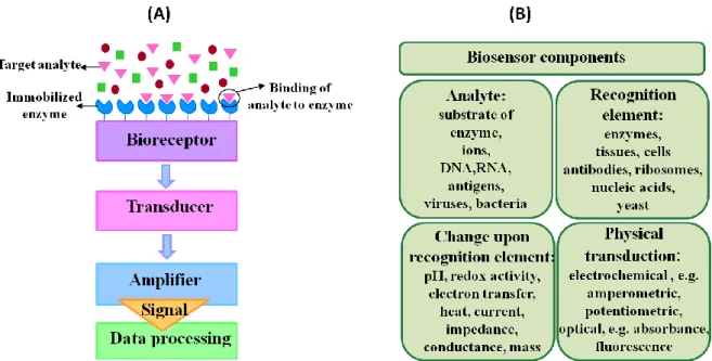
But what exactly is a biosensor? In its broadest sense, a biosensor is defined as an analytic device comprising three structural elements: a recognition element, a transducer, and an amplifier [Gri08]. The recognition component, which is any element sensitive to the analyte of interest, includes biological elements, ranging from tissues and cells to antibodies, enzymes, receptors, and nucleic acids, etc. Although biosensing devices employ a variety of recognition elements, electrochemical detection techniques have so far used predominantly enzymes. This is mostly due to their specific binding capabilities and biocatalytic activity [Egg02], [Dor03] and [Sch02].It is important to note that the biological recognition element is either integrated within or in close proximity to the transducer.

The transducer acts as an interface between the biological element and the amplifier, thereby performing a detector function. The main role of the transducer is to transform the signal originating from the interaction between the analyte and the recognition element into a recognizable and/or quantifiable physical output, for example, a current in an amperometric biosensor. Major types of transducers include electrochemical, optical, piezoelectric, and calorimetric transducers, which measure the changes in electric distribution, optical properties, mass, and thermal properties, respectively. Finally, the amplifier amplifies the transducer signal, which is displayed in a user-friendly way. Examples of these components along with a schematic view of a biosensor are illustrated in Figure 3.1.

The compilation given in Figure 3.1 helps one to understand which parameters change during a biological recognition event in a biosensor. This knowledge is fundamental for developing and optimizing biosensors. The choice of the transduction process and transduction material is dependent on this knowledge as well as the chemical approach to construct the sensing layer on the transducer surface.

The choice of the biological recognition element is the crucial decision that is taken when developing a novel biosensor design. Among the various recognition elements listed, enzymes are the most common and well developed, because they combine high chemical specificity and inherent biocatalytic signal amplification [Alk13].

(23)

14

Figure ‎3.1. Biosensor components : (A) Schematics of a biosensor set-up. (B) Examples for biosensor components.

Most biosensors use electrochemical detection for the transducer because of the low cost, ease of use, portability, and simplicity of construction. The reaction being monitored electrochemically, typically generates a measurable current, a measurable charge accumulation or potential, or alters the conductive properties of the medium between electrodes.

Depending upon the electrochemical property to be measured by a detector system, electrochemical biosensors may further be divided into conductometric, potentiometric and amperometric biosensors.

Conductometric devices are based on the measurement of changes in conductance between two metal electrodes as a result of a biochemical reaction, whereas potentiometric biosensors measure the potential difference between the anode and the cathode as a function of analyte concentration. Finally, amperometric biosensors measure the current change resulted by chemical reaction of electroactive materials while a constant potential is being applied. The amperometric biosensors are known to be more reliable, inexpensive and highly sensitive for the clinical, environmental and industrial purposes [Cha02].

The biosensor’s performance is usually experimentally evaluated based on its sensitivity, limit of detection (LOD), linear and dynamic ranges, reproducibility or precision of the response, selectivity and its response to interferences. Other parameters that are often compared include the sensor’s response time (i.e. the time after adding the analyte for the sensor response to reach 95% of its final value), operational and storage stability, ease of use and portability.

Figure 3.2 summarizes the key features of typical biosensors as well as several factors that are of additional importance for commercial devices.

(24)

Figure 3.2. List of key characters of a biosensor

Ideally, the sensing surface should be regenerable in order for several consecutive measurements to be made. For many clinical, food, environmental, and national defense applications, the sensor should be capable of continuously monitoring the analyte on-line.

However, disposable, single-use biosensors are satisfactory for some important applications such as personal blood glucose monitoring by diabetics.

3.1 Glucose sensors

The metabolic disorder of diabetes mellitus results in the deficiency of insulin and hyperglycemia and is reflected by blood glucose concentration higher or lower than the normal range of 80–120 mg dL⁻¹ (4.4–6.6 mM).The complications of battling diabetes are numerous, including higher risks of heart disease, kidney failure, or blindness. The World Health Organization (WHO) estimated the prevalence of diabetes worldwide to be approximately 9% of adults aged 18+ in 2014, announcing the disease as a leading cause of death and disability. Diagnosis and management of diabetes mellitus requires a tight monitoring of blood glucose levels, stimulating scientists to develop novel techniques through which patients can easily monitor their blood glucose levels. In particular, electrochemical glucose sensors have played a leading role in the move to efficient and easy-to-use blood sugar testing, alerting a person if their blood glucose levels are out of the normal range.

Electrochemical methods may be broadly grouped into two main categories: enzymatic and non-enzymatic approaches. While the former group is glucose specific, the latter is broadly adaptable and may be used to detect not only glucose, but also an assortment of other carbohydrates.

(25)

16

3.1.1 Enzymatic glucose biosensors

Glucose oxidase (GOD) is the most frequently employed enzyme for the development of electrochemical glucose biosensors [Pri03]. It possesses relatively higher selectivity for glucose and is able to withstand a wider range of pH, ionic strength and temperature, compared with any other enzymes, thus allowing less stringent conditions during the manufacturing process and relatively relaxed storage norms for use [Hel08].

The first glucose enzyme electrode introduced by Clark and Lyons of the Cincinnati Children’s Hospital [Cla62], relied on a thin layer of GOD entrapped over an oxygen electrode through the following reaction:

2 2

glucose+O GODgluconicacide+H O (3.1) A negative potential was applied to the platinum cathode for a reductive detection of the oxygen consumption

+ -

2 2

O +4H +4e 2H O _(3.2)

The first product based on the above technology was commercialized by the Yellow Spring Instrument company (YSI) using only 25 μL whole blood samples.

The entire glucose sensor market has grown rapidly since then, leading to the development of three generations of glucose biosensors. The differences among the generations are mainly concerned with the mode of electron communication between the redox centers of the employed enzyme and the electrode.

3.1.1.1 First-Generation biosensors

The first-generation glucose biosensors rely on the use of the natural oxygen and generation and detection of hydrogen peroxide (Eqs. 3.3 and 3.4) [Wan08]. The biocatalytic reaction involves the reduction of the flavin adenine dincleotide (FAD) in the enzyme by reaction with glucose which results in the reduced form of the enzyme (FADH2)

GOD (FAD) + glucose → GOD (FADH2) + gluconolactone (3.3) The reoxidation of the cofactor of GOD enzyme occurs in the presence of molecular oxygen, resulting in the formation of hydrogen peroxide (H2O2) as

GOD (FADH₂) + O₂→ GOD(FAD) + H₂O₂ (3.4) Thus, the rate of reduction of oxygen is directly proportional to the glucose concentration that is enumerated by either measuring the reduced oxygen concentration or increased concentration of hydrogen peroxide. Hydrogen peroxide thus produced as a byproduct is oxidized at a platinum (Pt) anode. The electric current is measured and correspondingly, the number of electrons transferred is directly proportional to the number of glucose molecules present.

H₂O₂→ O2+2H⁺+2e^- (3.5)

(26)

Measurements of peroxide formation have the advantage of being simpler, especially when miniaturized devices are concerned. However, the main problem with the first generation is electroactive interference, since a relatively high electric potential was needed to measure the H2O2. The high potential leads to endogenous reducing species, such as ascorbic and uric acids and some drugs, like acetaminophen [Wan08]. Another drawback is the oxygen dependence. As shown in Equation (3.4), the oxygen amount is a limiting factor (oxygen deficit) that controls the changes in sensor response and the upper limit of linearity.

3.1.1.2 Second-Generation bioensors

The abovementioned limitations of the first-generation glucose biosensors were overcome by using mediated glucose biosensors, i.e., second-generation glucose sensors.

Since the FAD redox center of the GOD is surrounded by a thick protein layer, the direct electron transfer from GOD to traditional electrodes is blocked. Various strategies have been employed to facilitate electron transfer between the GOD redox center and the electrode surface, such as employing nanomaterials, like gold nanoparticles (NPs) [Hol11] or CNTs [Woo14] as electrical connectors between the electrode and the FAD center. Covalent bonding of redox polymers is another approach to reduce the distance between the redox center of the polymers and the FAD center of the enzymes, which leads to a high current output and fast sensing response [Deg89].

The sensor performance was further improved by replacing oxygen with a nonphysiological electron acceptor (called redox mediators), that was able to shuttle electrons from the enzyme to the surface of the working electrode. The reduced mediator is formed instead of hydrogen peroxide and then reoxidized at the electrode, providing an amperometric signal and regenerating the oxidized form of the mediator. The reaction can be described as follows [Tog10]:

Glucose + GOD_(ox) → gluconic acid + GOD_(red) (3.6) GOD(red) + 2M(ox) → GOD(ox) + 2 M(red) + 2 H⁺ (3.7)

2M_(red) → 2M_(ox) + 2e⁻ (3.8)

where M(ox) and M(red) are the oxidized and reduced forms of the mediator. Artificial electron- carrying mediators, like ferrocene derivatives, ferricyanide, transition-metal complexes, etc.

are of particular interest, fitting the criteria for a good mediator, such as (i) reacting rapidly with the reduced enzyme while not reacting with oxygen, (ii) good electrochemical properties, like low operational potential, (iii) low solubility in aqueous medium, (iv) chemical stability in both reduced and oxidized forms [Bor12].

(27)

18

3.1.1.3 Third-Generation bioensors

In order to avoid complications offered by synthetic or natural mediators in second generation biosensors, new strategies for direct electron transfer between the electrode and active center of enzyme have been researched [Bar14] [Tas11], with the aim of developing highly selective and sensitive third-generation biosensors. The absence of mediators is the main advantage of such third-generation biosensors, leading to a very high selectivity (owing to the very low operating potential). However, as discussed earlier, critical challenges must be overcome for the successfulrealization of this direct electron-transfer route, owing to the globular structure of GOD with the active site, containing FAD/FADH2 redox cofactor, buried deep inside a cavity of ~13A°, which is a major hinderance for direct electron flow.

Figure 3.3 summarizes various generations of amperometric glucose biosensors based on different mechanisms of electron transfer, including the use of natural secondary substrates, artificial redox mediators, or direct electron transfer.

Figure ‎3.3. Summary of enzymatic glucose oxidation mechanisms , presented as (a) first, (b) second and (c) third generation sensors.

Although enzyme electrodes have witnessed massive progress and commercially available glucosemeters have opened broad opportunities for monitoring glucose level in real time [Gal15], notable drawbacks and disadvantages have been extensively interrogated, which originate mainly from the nature of GOD. Principally, the activity of enzyme is prone to be affected by temperature, acidity, and toxic chemicals, resulting in poor reproducibility and stability. Furthermore, laborious and complex protocols are required to immobilize enzyme on electrode, complicating the fabrication procedures and thus affecting their final performance [Urb15]. Because of the mentioned flaws, fabrication of enzyme-free glucose sensors has been continuously motivating research interests.

3.1.2 Electrochemical non-enzymatic glucose sensors

Various studies have been conducted to alleviate the drawbacks of enzymatic glucose sensors.

A non-enzymatic amperometric sensor for direct determination of glucose is an attractive