Properties of Random Fitness Landscapes and Their Influence on
Evolutionary Dynamics
- A Journey through the Hypercube -
Inaugural-Dissertation zur Erlangung des Doktorgrades
der Mathematisch-Naturwissenschaftlichen Fakult¨ at der Universit¨ at zu K¨ oln
vorgelegt von
Stefan Nowak
aus Abu Dhabi
Berichterstatter: Prof. Dr. Joachim Krug, Universit¨ at zu K¨ oln Prof. Dr. Anton Bovier,
Rheinische Friedrich-Wilhelms-Universit¨ at Bonn
Tag der m¨ undlichen Pr¨ ufung: 23.11.2015
Abstract
A fitness landscape is a theoretical concept in population genetics where a fitness value, which measures the reproductive success of an organism and is represented by a real number, is assigned to each genotype. Content of this thesis is the analytical and numerical study of stochastic models for fitness landscapes. The focus is on the landscape ruggedness and its influence on evolutionary dynamics. One proxy for the ruggedness is the number of local maxima, i.e., genotypes from which every mutation leads to lowered fitness. Another way to quantify ruggedness is the study of accessible paths, i.e., successions of mutations that increase the fitness monotonically. The question whether accessible paths exist can be interpreted as a kind of percolation problem. One model for evolutionary dynamics that will be used is the adaptive walk. In this model type, populations are treated as single entities that move through the space of genotypes according to certain probabilistic rules. They are closely related to both ruggedness measures as they follow accessible paths and terminate at local maxima. Furthermore, the individual-based Wright-Fisher model is used to study recombination of genotypes, interactions between individuals and the influence of the underlying fitness landscape on these mechanisms.
Kurzzusammenfassung
Fitnesslandschaften sind ein theoretisches Konzept der Populationsgenetik bei dem
jedem Genotypen eine reelle Zahl zugeordnet wird welche den reproduktiven Erfolg,
die Fitness, des entsprechenden Organismus repr¨ asentiert. Inhalt dieser Arbeit
ist die analytische und numerische Untersuchung von stochastischen Modellen f¨ ur
Fitnesslandschaften. Das Hauptaugenmerk ist auf die Rauigkeit der Landschaften
gerichtet und welche Auswirkungen diese auf evolution¨ are Prozesse hat. Rauigkeit wird
haupts¨ achlich auf zwei verschiedene Arten gemessen, n¨ amlich durch die Anzahl lokaler
Maxima, d.h. Genotypen von denen jede einzelne Mutation die Fitness verringert, und
durch das Vorhandensein von zug¨ anglichen Pfaden, d.h. Abfolgen von Mutationen
bei denen die Fitness monoton erh¨ oht wird. Letzteres kann auch als eine Art von
Perkolationsproblem aufgefasst werden. Evolution¨ are Prozesse werden zun¨ achst durch
sogenannte Adaptive Walks modelliert. In dieser Art von Modell wird eine Population als
einzelnes Objekt betrachtet, das sich nach bestimmten stochastischen Regeln durch den
Raum der Genotypen bewegt. Adaptive Walks folgen zug¨ anglichen Pfaden und enden
auf einem lokalen Maximum. Damit eng mit diesen Konzepten verbunden. Desweiteren
wird das individuenbasierte Wright-Fisher Modell in dieser Arbeit verwendet um die
Rekombination von Genotypen, Wechselwirkungen zwischen Individuen und den Einfluss
der zugrunde liegenden Fitnesslandschaft auf diese Mechanismen zu untersuchen.
Contents
1. Introduction 7
1.1. Evolution in a Nutshell . . . . 7
1.2. Basic Concepts . . . . 8
1.3. Structure of this Thesis . . . . 11
2. Fitness Landscape Models and their Properties 13 2.1. Hypercubes . . . . 13
2.2. Random Models for Fitness Landscapes . . . . 14
2.3. Fourier Decomposition . . . . 16
2.4. Local Maxima . . . . 20
3. Accessibility Percolation 31 3.1. HoC Model on Trees . . . . 32
3.2. HoC Model on the Directed Hypercubes . . . . 38
3.3. HoC Model on the Undirected Hypercube . . . . 45
3.4. RMF Model . . . . 50
3.5. NK Model . . . . 55
4. Adaptive Walks 59 4.1. Tree Approximation on the HoC Landscape . . . . 61
4.2. Adaptive Walks on the RMF Landscape . . . . 73
4.3. Adaptive Walks on the NK Landscape . . . . 75
5. Recombination and Disruptive Selection 83 5.1. Wright Fisher Model . . . . 83
5.2. Recombination . . . . 87
5.3. Frequency-Dependent and Disruptive Selection . . . . 95
6. Discussion 101 6.1. Summary . . . 101
6.2. Open Questions and Outlook . . . 104
A. Appendix 107
Bibliography 115
1. Introduction
Treating interdisciplinary problems is common practice in statistical physics. It is often the case that models and methods that were developed in this field in order to describe, for instance, interacting particles can also be applied to systems of interacting animals, persons, cars, companies, and so on. The corresponding branches of science related to these examples are biology, sociology, traffic engineering and economics, respectively.
In this thesis, evolutionary biology will be studied from a physicist’s perspective. This means that evolutionary processes, as described below, will be represented by idealized mathematical models. Many concepts that arise from this treatment are closely related to systems of interacting spins, but there are also many similarities to computer science.
This chapter explains these relationships between the different fields and introduces the concepts that will be used in this thesis.
1.1. Evolution in a Nutshell
Evolution is the change of lifeforms over generations. The basic ideas of the modern theory of evolution go back to the mid-19th century and Charles Darwin’s famous book On the Origin of Species [1]. Changes of an organism manifest in modified observable traits, the phenotype. Today it is known that these changes can be actually ascribed to modifications of the organism’s blueprint, the genotype. The genetic information is physically stored in Deoxyribonucleic acid (DNA) molecules that have a very complex structure. Simply speaking, the actual information corresponds to a certain arrangement of monomers, the nucleobases. Since there are four different types of nucleobases (cytosine, guanine, adenine, and thymine), an arrangement can also be represented by a sequence consisting of four possible letters (e.g., C, G, A, and T, corresponding to the initial letters of the nucleobases). When organisms reproduce, the genotype is inherited by the offspring. However, the offspring’s DNA sequence might differ slightly from that of its parent if mutations occur. They are caused, for instance, by replication errors of the DNA molecule. Therefore, also the offspring’s phenotype might be modified, which in turn can cause that it becomes worse or better adapted to its environment compared to the parent.
If a mutation in the offspring is beneficial, the organism will be more likely to survive and leaves on average more offspring with the mutated genotype to the next generation.
This reproductive success is measured by the fitness. In the long run, individuals with
high fitness will outnumber individuals with lower fitness, a process known as natural
selection. Thus the structure of the whole population will change on timescales of several
generations such that its overall fitness increases over time. This can lead to fixation of
8 Introduction
a genotype, i.e., only one genotype remains in the population while individuals carrying different genotypes go extinct.
Apart from mutation and selection, also other mechanisms play a role in evolution.
For instance, random fluctuations of the environment or the population affect the offspring production and hence the whole process. Another important example is the recombination of genotypes which provides a way to alter them independent of the occurrence of mutations.
1.2. Basic Concepts
1.2.1. Space of Genotypes and the Hypercube
In the description above, genotypes correspond to DNA sequences consisting of letters from the set {C, G, A, T}. In general, sequences can also be made of letters from different sets that are denoted as alphabets. Different systems can be modeled with different alphabets, e.g., proteins have an alphabet of 20 letters corresponding to different amino acids. Throughout this thesis, genotypes will be represented by binary sequences of fixed length L consisting of “letters” from the alphabet A = {0, 1}, i.e., the set of genotypes is given by A
Land consists of 2
Lsequences. The position of a letter in the sequence is called locus. A common biological interpretation is to denote the presence or absence of a certain mutation by one and zero, respectively. The loci correspond then to different possible mutations. In the same manner, genes that can occur as two different alleles or in two different states can be distinguished. A mutation at a certain locus corresponds to the change of a zero to a one or vice versa.
As a distance measure between two elements σ and τ of {0, 1}
L, it is convenient to use the Hamming distance
d(σ, τ ) = L −
L
X
i=1
δ
σi,τi, (1.1)
where δ
i,jis the Kronecker delta. This is nothing but the number of loci at which σ and τ differ. Therefore, it is obvious that the Hamming distance is not restricted to the choice A = {0, 1} as a reasonable metric. However, with this particular alphabet choice, an element σ ∈ {0, 1}
Lcan be interpreted as a point of R
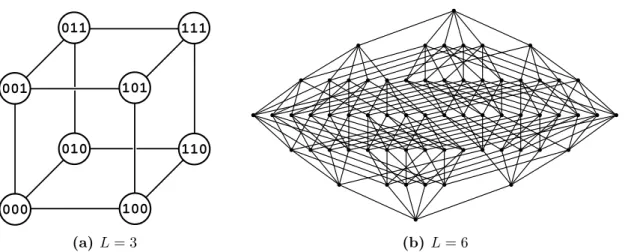
Lthat is located on a corner of the L-dimensional unit cube as shown in figure 1.1(a). For this reason, the undirected graph H
L2, where vertices correspond to sequences and edges correspond to two sequences at Hamming distance 1, is called hypercube graph or simply hypercube.
Basic properties of this type of graph will be explained in section 2.1. Note that the
graph topology does not depend on the particular choice of letters but only on their
number. The generalization H
Lato alphabets of arbitrary size a = |A| is called Hamming
graph.
Section 1.2 – Basic Concepts 9
(a)L= 3 (b)L= 6
Figure 1.1. Examples of hypercube graphs. Figure (a) is arranged in a way that demonstrates the cube structure. The graph in figure (b) can be arranged to a cube as well when embedded into 6-dimensional space, which is not obvious though.
1.2.2. Fitness Landscapes
Fitness is a measure for the reproductive success of an individual. It quantifies the individual’s contribution to the gene pool of a population in succeeding generations.
Therefore, fitness can be identified with the average number of offspring it leaves to the next generation. Independent of the interpretation, the fitness will be represented by a real number. Assuming that the genotype contains all information about the fitness of an individual, at least with respect to a given environment, there is a mapping w : H
L2→ R from the space of genotypes to the fitness which is called a fitness landscape [2–4].
Even though there exist some empirical fitness landscapes for small values of L [3], the mechanism in which the genotype is translated into a fitness value is highly complex and far from being understood. For this reasons, models for fitness landscapes usually use random variables. Different variants that will be used in this thesis are defined in section 2.2.
Epistasis and Ruggedness
Landscapes on countrysides look very different in terms of ruggedness, e.g., they can be
very plain, have gentle hills or be completely jagged. Ruggedness is usually associated
with an increased number of mountain peaks. Hiking through such a landscapes often
requires to go up- and downhill alternatingly. As the name suggest, fitness landscape can
be thought of as a high-dimensional but discrete analogue by interpreting the fitness as
a height profile. Mountain peaks correspond to local maxima, i.e., genotypes from which
every single mutation leads to lower fitness. In the same way it is exhausting for a hiker
to walk through a rugged landscape, it is difficult for a population to evolve in a rugged
fitness landscape. Properties of fitness landscapes in terms of the local maxima and the
existence of fitness-monotonic paths will be discussed in chapter 2 and 3, respectively.
10 Introduction
Related to ruggedness is the concept of epistasis [5]. It means that the effect of a mutation at a certain locus is influenced by the state of other loci, the genetic background.
In the absence of epistasis, a mutation at a certain locus will lower or increase the fitness by an amount that is independent of the state of other loci. Such a landscape is called additive, since the total fitness is simply the sum of the contributions from each locus.
One distinguishes between different types of epistasis: Magnitude epistasis denotes the situation where only the strength of a mutational effect on the fitness is dependent on other loci, but not whether mutations are generally beneficial or deleterious. Sign epistasis [6], on the other hand, means that also the algebraic sign of a mutational effect varies, i.e., beneficial mutations can turn into deleterious ones (or vice versa) if mutations at different loci occur beforehand. High ruggedness is associated with a frequent occurrence of sign epistasis. Reciprocal sign epistasis [7] between two loci i and j means that they influence each other sign epistatically, i.e., j has an sign epistatic effect on i and vice versa.
Landscapes Outside Biology
The concept of a fitness landscape can also be found in fields different from biology. A more general terminology is value landscape, a mapping C → R from the configuration space C of a system to the real numbers. The configuration space does not need to be a Hamming space, but it should include the notion of a neighborhood to justify the term
“landscape”.
This applies, for instance, to most physical systems where the energy plays the role of the (negative) fitness. In analogy to biological populations that are driven into states with high fitness, physical systems evolve into states with low energy. Metastable states correspond to local minima of the energy landscape. The analogy can be taken even further for systems of interacting spins [8]. If there are L spins with two possible orientations −1 and +1, the configuration space C = {−1, +1}
Lis isomorphic to the hypercube, where spin flips correspond to mutations.
Value landscapes also play an important role in computer science and optimization.
On the NK landscape, a model for fitness landscapes that is also going to be used in this
thesis, it is in general an NP-complete problem to determine whether the maximal fitness
among all genotypes is below a given threshold [9]. For that reason, it is commonly used
as a benchmark for optimization algorithms. Another famous example is the traveling
salesman problem, where the task is to find the shortest possible route that visits each
city on a given list of n cities. The configuration space is then given by the set of
permutations of cities while the (negative) fitness corresponds to the length of the route
defined by a permutation [10, 11]. Similar to the situation on the NK landscape, it is
an NP-hard problem to solve the traveling salesman problem [12] and hence there exist
no efficient algorithm to find the global minimum of the corresponding landscape.
Section 1.3 – Structure of this Thesis 11
1.2.3. Evolutionary Dynamics
Evolutionary dynamics determines how the frequency of genotypes within a population changes over time. Models used to simulate evolutionary dynamics are often defined as stochastic processes. Since also the underlying fitness landscapes are modeled with random numbers, the outcome of a realization of the system is influenced by two different types of stochasticity. Certain questions can only be answered in terms of probabilities and averages.
In this thesis, two types of models for evolutionary dynamics are studied. They are both rather simple, yet they show interesting and non-trivial behavior. One type, a version of the Wright-Fisher model [13, 14], is individual based. Simply put, individuals produce offspring according to their fitness and mutations occur during this reproduction process with some probability, i.e., it corresponds basically to the scenario described in section 1.1. The dynamics will also be extended by the recombination of genotypes as well as with the competition between individuals. A detailed description of the model and its extensions will be given in chapter 5. The other type of dynamics, adaptive walks, is even simpler and arises in certain limits of the more general Wright-Fisher dynamics.
Here one does not distinguish between individuals. Populations are rather treated as single objects that “walk” over the fitness landscape according to certain probabilistic rules. They will be studied in chapter 4.
Note that evolutionary dynamics plays also a role outside biology. For optimization problems, like the above mentioned traveling salesman problem, it is not feasible to search the whole configuration space. These and similar problems can be treated by so-called genetic algorithms [15] that mimic the behavior of a population evolving on the respective landscape. One can find particularly fit states with this method, which may suffice for practical applications, but in general one does not find the fittest state in large systems.
1.3. Structure of this Thesis
Chapter 2 begins with the recalling of basic properties of hypercube graphs and the definition of fitness landscapes models that are used in this thesis. Properties of these models will be discussed as well in this chapter with two different approaches. Firstly, a discrete analogue of Fourier analysis yields information about epistatic interactions on the landscape. Secondly, the study of local maxima serves as a direct proxy for landscape ruggedness. In particular, it will be studied how the scheme of epistatic interactions, which can be explicitly defined in the NK model, affects the number of maxima.
In chapter 3, accessibility percolation will be studied, a type of percolation problem that addresses paths to the global maximum such that the fitness is in ascending order along the paths. These accessible paths are favored to be taken by a population due to natural selection. In contrast to local maxima, which are local features of the landscape, accessible paths cross the whole landscape and are therefore global features.
Adaptive walks will be studied in chapter 4. Here it will be shown how the landscape
properties influence the dynamics on it. For specific landscape models, a large class of
12 Introduction
adaptive walks can be studied solely analytically. More sophisticated models require numerical simulations. Similar to the above-mentioned local maxima, the influence of epistatic interactions on the behavior of adaptive walks will be studied as well.
When the attention will be turned to the Wright-Fisher dynamics in chapter 5, results are almost entirely obtained by numerical simulations. The focus will be on two extensions of the basic dynamics, namely recombination and disruptive selection. In both cases, the underlying fitness landscape has crucial influence on the dynamics. In particular, the question of whether these mechanisms are advantageous for a population depends strongly on the landscape ruggedness.
A precise explanation of models and methods will be given in the beginning of each
chapter. Apart from that, rather standard notation will be used throughout this thesis,
but in order to avoid confusion and ambiguities it will also be explained in appendix A.1
on page 107.
2. Fitness Landscape Models and their Properties
2.1. Hypercubes
The hypercube graph, independently of a fitness landscape on top of it, has already interesting properties. Some of them will be recalled in the following.
• Since every vertex corresponds to a binary sequence of length L, there are 2
Lvertices in total. Each of them has a degree of L and hence there is a total of L · 2
L−1edges in the graph.
• The number of sequences at distance d to a reference sequences σ is given by
Ld.
• The hypercube is a bipartite graph, i.e., the vertices can be divided into two disjoint sets such that there are no edges within a set. For instance, the sequences can be allocated according to whether they contain an odd or even number of ones.
• The hypercube is a Hamiltonian graph, i.e., there exist cycles in the graph that visit each vertex exactly once [16]. A famous example of such a cycle is the Gray code [16, 17].
• A path through the hypercube that contains n vertices can be represented by the starting vertex and a string of length n − 1 consisting of numbers in {1, 2, . . . , L}. The number at the i-th position corresponds to the locus which is flipped from 0 to 1 or vice versa in the i-th step. For instance, the path
(0, 0, 0) → (0, 1, 0) → (0, 1, 1) → (1, 1, 1) → (1, 1, 0)
can be represented by the string 2313. The path is self-avoiding if and only if there is no substring that contains all occurring numbers an even number of times.
• Between two vertices σ and τ at distance d = d(σ, τ ) there are d! shortest paths that correspond to the number of possible successions in which the differing loci of σ and τ can be flipped.
• The number of shortest paths between two sequences with d(σ, τ ) that share exactly
k − 1 interior vertices (i.e., vertices different from σ and τ ) is equal to the number
T (d, k) of permutations with k components [18], a number that appeared in the
mathematical literature before, independently of the hypercube context [19, 20].
14 Fitness Landscape Models and their Properties
Though no formula exist for T (d, k) in simple closed form, it was proven in [18]
that
d!
1 − O
1 d
≤ T (d, 1) ≤ d! , (2.1)
which means that most of the paths do not share any interior vertices for large d.
• The total number of self-avoiding paths (that are not required to be shortest) between two sequences σ and τ is not known exactly. However, the question was mainly addressed to antipodal vertices, i.e., to the case d(σ, τ ) = L. The corresponding number a
Lwas computed by simple enumeration of all paths up to L = 5 [21]. As a
Lgrows very rapidly, this is not possible anymore for L > 5. In [22] it was found that a
Lgrows double-exponentially, or more precisely, that
L→∞
lim
log(log a
L)
L = log 2 . (2.2)
2.2. Random Models for Fitness Landscapes
2.2.1. House-of-Cards Model
The House-of-Cards (HoC) model [23, 24] is in some sense the simplest version of a random fitness landscape model. For each genotype σ, the fitness w(σ) is a random number drawn independently from a continuous probability distribution. If the landscape is interpreted as an energy landscape, the HoC model is the analogue of Derrida’s random energy model [25, 26].
2.2.2. Rough-Mount-Fuji Model
The Rough-Mount-Fuji (RMF) model [27, 28] is a simple extension to the HoC model in the version used here. It introduces a global gradient to the landscape, i.e., the fitness is given by
w(σ) = η(σ) + s d(σ, σ) ˜ , (2.3) where η is a HoC landscape, ˜ σ is some reference sequence and s is a constant. Given that s > 0, the fitness increases on average the further away σ is from ˜ σ. The strength of the increase is controlled by the slope parameter s. The term η(σ) will be referred to as the random part of the fitness, the second term as the additive part.
2.2.3. NK Model
Basic idea of this model is that total fitness associated with a genotype is made up of several contributions, where each contribution depends only on 1 ≤ K ≤ L loci of the genotype [29]. Fitness is given by
w(σ) =
L
X
i=1
η
iσ
bi,1, . . . , σ
bi,K, (2.4)
Section 2.2 – Random Models for Fitness Landscapes 15
1 2 3 4 5 6 7 8 9 2
1 3 4 5 6 7 8 9
(a) Adjacent
1 2 3 4 5 6 7 8 9 2
1 3 4 5 6 7 8 9
(b) Block
1 2 3 4 5 6 7 8 9 2
1 3 4 5 6 7 8 9
(c)Random
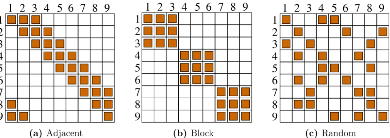
Figure 2.1. Illustration of the classic interaction patterns forL= 9 andK= 3. A filled square in rowi and columnj means thatVi containsj.
where for each i and each τ ∈ {0, 1}
Kthe contribution η
i(τ ) is a random number independently drawn from some continuous distribution. In other words, the η
iare independent HoC landscapes of size K. The matrix b
i,jdetermines the interactions between different loci, often referred to as the genetic neighborhood. The order of the arguments of η
idoes not affect landscape properties and hence the interaction scheme can be defined equivalently as sets
V
i= {b
i,1, b
i,2, . . . , b
i,K} . (2.5) There are almost no constraints on these sets apart from their number being equal to L and that |V
i| = K as well as i ∈ V
ifor all i. The last condition ensures that each locus occurs in at least one set, but there is actually no mathematical or biological reason to assume that the number of contributions is equal to L or that each contribution depends on the same number K of loci. Note that in the literature the parameter K is often defined in a way that the random functions η
idepend on K + 1 rather than K loci.
Furthermore, the genotype length is often denoted by N rather than L (and hence the name “NK model” with regard to the parameters N and K).
Interaction Patterns
As mentioned above, there are lots of degrees of freedom concerning the interaction sets V
i. The most common choices in the literature, which will also be used in this thesis, are the following (see figure 2.1 for an illustration):
Adjacent. Tupels of K adjacent loci interact with each other, i.e., the interaction sets are given by
V
i= {i, i + 1, . . . , i + K − 1} , (2.6)
where the elements have to be read modulo L.
16 Fitness Landscape Models and their Properties
Block. The sequence is divided into L/K blocks, where each locus interacts with all other loci within the same block, but not with loci from other blocks. Interaction sets are given by
V
i=
K i
K
− 1
+ 1, K i
K
− 1
+ 2, . . . , K i
K
− 1
+ K
, (2.7) where dxe is the ceiling function. The sequence length L has to be an integer multiple of K.
Random. The set V
icontains i as well as K − 1 randomly chosen elements from {1, . . . , i − 1, i + 1, . . . , L}.
Depending on the property under consideration, the interaction scheme has more or less influence on the landscape. There are also certain characteristics, like the Fourier spectrum (see section 2.3), that are completely independent of the particular choice of the scheme. Other properties, e.g. the number of local maxima, are highly susceptible to this choice as will be shown later.
2.3. Fourier Decomposition
2.3.1. Expansion in Eigenfunctions of the Graph Laplacian
Any function w : H
L2→ R can be decomposed into eigenfunctions of the graph La- placian ∆ of the hypercube [30–32]. This transformation can be thought of as a discrete analogue of a Fourier transformation. The graph Laplacian reads ∆ = A − L1
2Lwhere 1
nis the n × n identity matrix and
A
σ,τ=
( 1 if d(σ, τ ) = 1 ,
0 otherwise , (2.8)
is the adjacency matrix of the hypercube. Treating ∆ as an operator, its effect on a function w is given by
∆w(σ) = X
τ∈HL2
A
σ,τw(τ ) − L w(σ) = X
τ∈Uσ
w(τ ) − L w(σ) , (2.9) where U
σ=
τ ∈ H
L2| d(σ, τ ) = 1 is the set of neighbors of σ. The eigenfunctions of ∆, also known as Walsh functions, are given by
φ
I(σ) = 2
−L/2· (−1)
Pi∈Iσi, (2.10) where the set I = {i
1, . . . , i
p} of indices is a subset of {1, . . . , L}. The corresponding eigenvalues λ
p= −2p do only depend on p and hence they have a rather large degeneracy of
Lp. With the inner product defined by hφ, ψi = X
σ∈HL2
φ(σ) ψ(σ) , (2.11)
Section 2.3 – Fourier Decomposition 17
the Walsh functions form an orthonormal basis such that a function w can be expressed as a linear combination
w(σ) =
L
X
p=0
X
i1<···<ip
a
i1,...,ipφ
{i1,...,ip}(σ) . (2.12)
This transformation is sometimes also called Walsh transformation [33, 34]. If the genotypes are represented by sequences from s ∈ {−1, +1}
Lrather than σ ∈ {0, 1}
L, which corresponds to a transformation s = 2σ−1, the Walsh functions take a particularly simple form proportional to products s
i1· · · s
ip. Strings consisting of −1 and +1 can be naturally interpreted as configurations of one-dimensional spin systems. Therefore, the Fourier transformation (2.12) has the same form as the energy of a superposition of diluted p-spin glasses [25, 35]:
w(s) = w
0+
L
X
i=1
h
is
i+
L
X
p=2
X
i1<···<ip
J
i1...ips
i1· · · s
ip, (2.13)
where h
iis a random “magnetic field” and J
i1...ipare random “coupling constants”.
2.3.2. Amplitude Spectrum
The importance of the Fourier transformation is based on the exposure of interactions between loci. A coefficient a
i1...ipfor p > 1 is only non-zero, if all loci i
1, . . . , i
pinteract epistatically with each other. Its absolute value tells how strong the interaction is. On the other hand, the first-order coefficients a
itell how strong the non-epistatic influence of locus i is, i.e., how strong the average effect of a mutation at locus i is, independent of the state of other genes.
The spectrum B
pis a way to quantify the influence of certain orders p of interactions.
Among other similar definitions, it can be defined as B
p=
P
i1<···<ip
|a
i1,...,ip|
22
LCov(w) + P
Lq=1
P
i1<···<iq
|a
i1,...,ip|
2, p ∈ {1, . . . , L} , (2.14) where h. . .i means averaging over realizations of the landscape and
Cov(w) = 4
−LX
σ,τ∈HL2
h
w(σ) w(τ )
− w(σ)
w(τ ) i
(2.15)
is the mean covariance of the fitness. The amplitude spectrum B
pis also related to the autocorrelation function R
dvia a linear transformation [30].
In the NK model, there are only epistatic interactions between loci i
1, . . . , i
pif they are
all contained in at least one interaction set V
j. Since these sets contain only K elements,
it is obvious that a
i1...ip= 0 for p > K and hence the sum over p in equations (2.12)
18 Fitness Landscape Models and their Properties
and (2.13) terminates at p = K . By definition, this implies that B
p= 0 for p > K . In fact, the spectrum can be computed explicitly [32] and is given by
B
(NK)p= 2
−KK
p
, (2.16)
independent of the underlying interaction scheme of the NK landscapes. The spectrum of the HoC model is obtained from (2.16) by setting K = L. One finds for the RMF model that
B
p(RMF)= N s
2δ
p,1+ 4 Var(η) 2
−N LpN s
2+ 4 Var(η) , (2.17)
where Var(η) is the variance of the random component of the landscape. This spectrum corresponds to a superposition of a HoC and an additive landscape.
2.3.3. The Rank
The rank R was introduced in [36] to study interaction patterns of NK landscapes.
Among other equivalent definitions, it can be defined as the number of non-zero coefficients in the Fourier expansion (2.12). Therefore, it is not applicable to HoC or RMF landscapes, since the random term of the fitness causes that all coefficients are non-zero which leads to R = 2
L.
For NK landscapes, however, it will turn out to be very useful for the quantification of interaction schemes since the rank, unlike the spectrum, is strongly influenced by them.
For the actual calculation of the rank, it is convenient to use the equivalent definition R = |V| =
L
[
i=1
P (V
i)
, (2.18)
where P (S) and |S| denote power set and counting measure, respectively, of a set S.
The set V = S
i
P (V
i) contains all sets of indices of non-zero coefficients in the Fourier expansion.
The maximal rank of a classic NK landscapes with fixed L and K is reached when the overlap between interaction sets is as small as possible. Each interaction set V
ican contribute at most
Kmsubsets of size m to the union V. Since the empty set and the L unit sets are always contained in V, an upper limit for the rank is given by
R
max= 1 + L + L
K
X
m=2
K m
= 1 + L (2
K− K) . (2.19)
This is a sharp bound and hence one can construct interaction schemes that reach this
rank. However, not all values of L and K allow for such patterns with R = R
max. It
can be shown that such a scheme exists if an (L, K )-packing design, an object known
in combinatorial design theory, exists [36]. The actual rank for the different standard
interaction patterns was computed in [37] and will be presented in the following.
Section 2.3 – Fourier Decomposition 19
Rank of Block Interactions
It is particularly easy to calculate the rank for blockwise interactions, because two contributions P(V
i) and P (V
j) to equation (2.18) are always either equal or disjoint apart from the empty set. The number of disjoint contributions is equal to the number L/K of blocks and each contribution contains 2
Kelements. Taking into account that the empty set is only counted once, the rank is given by
R
block= L
K 2
K− 1
+ 1 . (2.20)
Rank of Adjacent Interactions
In the adjacent case, the interaction set V
icontains the integers from i to i + K − 1, but all elements are taken modulo L. Therefore, one can interpret the elements as particle positions on a one-dimensional lattice of length L with periodic boundary conditions.
By definition, the particles are strung together and form a cluster of size K. Therefore, a set S is contained in V if and only if all particle positions in S can be found in an interval of size K, or equivalently, if there is a gap of size L − K or larger. The rank is nothing but the number of sets contained in V and thus it is equal to the number of ways one can put an arbitrary amount of indistinguishable particles on a periodic lattice such that a gap of size L − K emerges.
For K < (L + 1)/2, there can be only one gap of the required size such that it is straightforward to enumerate all valid particle configurations. One has exactly L possibilities to choose the first occupied site after the gap. Then the K − 1 subsequent sites can be either occupied or empty, giving a factor of 2
K−1to each position of the first occupied site. Finally, the configuration without any particles has to be included as well. This leads to
R
adj= 1 + L 2
K−1, if K < (L + 1)/2 . (2.21) If K is too large, there may be several gaps. In this case, the factor 2
K−1also includes configurations with another gap of the required size. As a consequence, these configurations are counted more than once by the enumeration procedure described above and equation (2.21) overestimates the actual rank.
Rank of Random Interactions
By definition, the actual rank for random interaction is a stochastic quantity. Its mean value will be calculated in the following. Let S be an arbitrary subset of {1, . . . , L} with
|S| = m and p
mthe probability that S is contained in V. Unit sets as well as the empty set are always contained and hence p
0= p
1= 1. For m > 1 one finds
p
m= P [S ∈ V ] = P [∃ i: S ⊂ V
i]
= P [∃ i ∈ S : S ⊂ V
i] + P [∃ i / ∈ S : S ⊂ V
i]
=
1 − (1 − q
m)
m+
1 − (1 − q
0m)
L−m, (2.22)
20 Fitness Landscape Models and their Properties
where
q
m=
K−1 m−1
L−1 m−1
= (K − 1)! (L − m)!
(L − 1)! (K − m)!
and
q
0m=
K−1 m
L−1 m
= q
mK − m L − m
are the probabilities that S ⊂ V
i, conditioned on i ∈ S and i / ∈ S, respectively. When K is sufficiently smaller than L, the probabilities q
mand q
0mare very small and one can use the approximation (1 − x)
n≈ 1 − nx in equation (2.22) that yields
p
m≈ m q
m+ (L − m) q
0m= K q
m= K! (L − m)!
(L − 1)! (K − m)! . (2.23) Finally, the mean rank is obtained by summing over all possible sets which reads
E [R
rnd] = X
S⊂{1,...,L}
P [S ∈ V ] = 1 + L +
K
X
m=2
L K
p
m≈ 1 + L +
K
X
m=2
L K
K! (L − m)!
(L − 1)! (K − m)!
= 1 + L(2
K− K) = R
max. (2.24)
Since the average rank is close to the upper limit, it is safe to assume that the fluctuations around E [R
rnd] are very small.
2.4. Local Maxima
Local maxima of a fitness landscape are those sequences that only have neighbors with lower fitness. They play an important role for evolutionary dynamics, because individuals whose genotype is a local maximum cannot improve their fitness by a single mutation which makes it hard to escape from them. The total number or density of local maxima is an important measure for the ruggedness of the landscape. Furthermore, it is also important to know how the maxima are distributed over the landscape as their positions are correlated. For example, it is by definition not possible that two neighboring genotypes are both maxima, but apart from that they tend to form clusters in most models.
2.4.1. HoC Model
In this model, the independence of fitness values facilitates the study of local maxima
by a large amount. A sequence σ being fitter than all of its L neighbors is equivalent
Section 2.4 – Local Maxima 21
to w(σ) being the largest of L + 1 i.i.d. random variables. Since each random variable has the same chance to be the largest, the probability P
maxthat a genotype is a local maximum is independent of the underlying fitness distribution and given by
P
max= 1
L + 1 . (2.25)
Multiplying P
maxwith the total number of genotypes gives the expected number of local maxima
E [N
max] = 2
LL + 1 . (2.26)
The fitness h of a local maximum can be obtained due to the fact that it is the largest of L + 1 random variables as well. Its cumulative distribution function (CDF) reads
F
max(x) = F (x)
L+1, (2.27)
where F is the overall fitness distribution function. In contrast to N
max, the average height E [h] of local maxima and even the scaling with L depends on the distribution.
One can, however, always scale the fitness values to the uniform distribution which yields E [F(h)] = 1 − 1
L + 2 . (2.28)
Moreover, one can compute the probability P
max,2that two sequences σ and τ with d(σ, τ ) = 2 are both local maxima. They do not have an independent chance to be local maxima as their neighborhoods share two common vertices. The number of genotypes involved in this situation is 2L and hence both σ and τ have a probability of 1/2L to be the largest of them. Given that, for instance, σ has the largest fitness, the probability that τ is larger than its neighbors is still 1/(L + 1) and hence
P
max,2= 2 · 1 2L · 1
L + 1 = 1
L (L + 1) > P
max2, (2.29) where the factor 2 is due to the interchangeable roles of σ and τ . The result implies that there is a weak enhancement in probability to find local maxima at distance 2 to other maxima, even though fitness values are uncorrelated. For d(σ, τ ) > 2, however, σ and τ have an independent chance to be local maxima since they do not share any common neighbors.
2.4.2. RMF Model
In contrast to the other models, the RMF model is not isotropic in the sense that
the probability P
maxfor a sequence σ depends on its distance d(σ, σ) to the reference ˜
sequence. Suppose d(σ, σ) = ˜ d, then the fitness w(σ) has according to equation (2.3) the
cumulative distribution function F(x − s d), where F is the CDF of the random part of
the fitness. Furthermore, σ has d neighbors that are located closer to ˜ σ (downhill) and
22 Fitness Landscape Models and their Properties
L − d neighbors that are farther away (uphill). Obviously, all down- and uphill neighbor must have smaller fitness than w(σ) if σ is a local maxima. The probability for this is given by F [w(σ) − s (d − 1)]
d· F [w(σ) − s (d + 1)]
L−d. Integrating over σ’s possible fitness values yields
P
max(d) = Z
∞−∞
f(x) F (x + s)
dF (x − s)
L−ddx . (2.30) Since F (x + s) > F (x − s), one can see immediately that P
max(d) increases with d. The corresponding probability for a randomly chosen genotype is accordingly given by
P
max= 2
−LL
X
d=0
L d
P
max(d) = 2
−LZ
∞−∞
f (x) [F (x + s) + F (x − s)]
Ldx . (2.31) Equations (2.30) and (2.31) cannot be expressed in simple closed form for arbitrary distributions of the random part, but it was shown in [38] that the leading order behavior of P
maxis given by
P
max= 1
L + 1 − s
2L (L − 1) 2
Z
∞−∞
f (x)
3F (x)
L−2dx + O s
4. (2.32)
Furthermore, a couple of special cases were presented in [38] where P
max(d) or P
maxcan be computed asymptotically exact. An interesting example is the Weibull distribution
F (x) =
1 − e
−xνθ(x) , (2.33)
where θ(x) is the Heaviside function. It was shown that the asymptotic behavior is given by
P
max∼
1/L for ν < 1 ,
esh
(
1−e−2s)
L+1−(
1−e−s)
L+1i2L(L+1)
+
1−(
1−e−scoshs)
(L+1) coshs
for ν = 1 ,
1 L
exp
−ν s (log L)
1−1/νfor ν > 1 .
(2.34)
The result for ν < 1 corresponds to the HoC model, which means that the fitness values are dominated by the random part if its distribution decays more slowly than exponentially and L is large. On the contrary, for ν ≥ 1 the slope s has also for L → ∞ a notable effect.
2.4.3. NK Model
Obtaining results on the number of maxima in the NK model is a challenging task.
Obviously, for a sequence to be a local maximum, each mutation must result in lower
fitness which makes things complicated due to the change of several contributions at
once. Nevertheless, one can write down the corresponding probability and the expected
height of a local maximum, at least formally.
Section 2.4 – Local Maxima 23
Suppose an NK landscape with interaction sets V
i, a sequence σ with fitness w(σ) =
L
X
i=1
x
i,
where x
i= η
iσ
bi,1, . . . , σ
bi,Kare the contributions to the total fitness and let f be the probability density function (PDF) of the contributions, i.e., the distribution of the total fitness is given by the L-fold convolution of f . When a mutation at the i-th locus occurs, the set of indices of affected contributions is given by
U
i=
j ∈ {1, . . . , L} | i ∈ V
j, (2.35) i.e., all contributions x
jwith j ∈ U
iwill be altered to a new value x
0j. If σ is a local maximum, the sum over the new values has to be smaller than the sum over the old values. Assuming that the x
iare fixed, the probability for this can be written as
P
X
j∈Ui
x
0j< X
j∈Ui
x
j
= ˜ F
|Ui|X
j∈Ui
x
j, (2.36)
where ˜ F
nis the cumulative distribution function corresponding to the probability density defined by the convolution
f ˜
1(x) = f (x) , f ˜
n+1(x) = Z
∞−∞
dz f (z) ˜ f
n(x − z) , (2.37) i.e., ˜ f
nis the PDF of P
j∈Ui
x
0jfor |U
i| = n. Note that mutations at different loci yield different sets of new contributions and hence, as long as the vector x = (x
1, . . . , x
L) of old contributions is fixed, the probabilities in equation (2.36) are independent for different i. Therefore, the actual probability that σ is a local maximum is obtained by taking the product over all i and integrating over all values of x. This reads
P
max= Z
RL
d
Lx
L
Y
i=1
h
f (x
i) ˜ F
|Ui|X
j∈Ui
x
ji
. (2.38)
Note that a similar expression, which was restricted to Gaussian random numbers, was derived in [36].
The integrand of equation (2.38) is the joint probability of being a local maximum and probability density of the contributions. Using the definition of conditional probabilities, the expected fitness h of a sequence, given that it is a maximum, reads
E [h] = 1 P
maxZ
RL
d
Lx
L
X
k=1
x
k!
LY
i=1
h
f (x
i) ˜ F
|Ui|X
j∈Ui
x
ji
. (2.39)
In most cases, however, neither equation (2.38) nor (2.39) can be expressed in simple
closed form. It is even worse for random interactions since P
maxand E [h] depend on
24 Fitness Landscape Models and their Properties
the precise realization of the interaction scheme. If the interaction scheme is chosen randomly, P
maxwill be a random variable as well. One might also want to perform the average over realizations of the U
i, but this is obviously a difficult task. In the following P
maxdenotes nevertheless this average rather than the actual variable if not stated otherwise, i.e., it is defined as the probability that a randomly chosen genotype is a local maximum in a landscape with a randomly chosen interaction pattern. The same applies to E [h].
Block Interactions
In the block model, in contrast to other interaction schemes, it is straightforward to compute the mean number of maxima [39, 40] and even the probability to have two maxima at certain distances [37]. A sequence σ is a local maximum if and only if each of the sub-landscapes induced by the block structure has a maximum at the corresponding sub-sequence. There are L/K blocks, each block’s sub-landscape is a HoC landscape of size K, and hence
P
max= 1
K + 1
KL. (2.40)
Given that σ is a maximum, the probability that a second sequence τ at distance d(σ, τ ) = 2 is also a maximum depends on two things: Firstly, both loci in which σ and τ differ have to be within the same block, otherwise the condition that each block has to be a maximum by itself cannot be fulfilled. If τ is randomly chosen among the second- nearest neighbors of σ, the probability for this is (K − 1)/(L − 1). Secondly, the two alterations of the sequence have to lead to another maximum of the sub-landscape in the corresponding block. This happens with probability 1/K according to equation (2.29).
Combining both considerations, the probability that two randomly chosen sequences at distance 2 are both maxima is given by
P
max,2= K − 1
K (L − 1) P
max, (2.41)
which is very large compared to P
max2.
In principle, one can extend this method to sequences at arbitrary distance d. It is required that there are either no or at least two differing loci in each block. In case d = 3, all differing loci have to be in the same block and hence the calculation is completely analogous to the previous one. It yields
P
max,3= (K − 1) (K − 2)
(K + 1) (L − 1) (L − 2) P
max= K (K − 2)
(K + 1) (L − 2) P
max,2. (2.42)
For d > 3, a laborious case analysis is required since the differing loci can be distributed
over the blocks in various ways.
Section 2.4 – Local Maxima 25
Distribution K λ
KE [h]/L Ref.
Gamma(2, 1) 2 0.56457. . . 2.88039. . . [43]
Exp(1) 2 0.56268. . . 1.61651. . . [43]
Exp(1) 3 0.61140. . . 1.86367. . . [43]
Negative Exp(1) 2 0.57695. . . −0.48097. . . [41]
Gamma(1/2, 1) 2 0.56062. . . 0.92242 . . . [37], this thesis
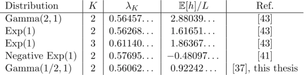
Table 1. Exactly known values for the asymptotics of the mean number and height of local maxima in the NK model with adjacent interactions. The constant λK is defined in equation (2.43).
General Phenomenology
Many quantities on the NK landscape with adjacent or random interactions behave qualitatively like the model with block interactions. It is known for adjacent interactions that the number of maxima grows exponentially with sequence length L, or more precisely that
L
lim
→∞log P
maxL = log λ
K, (2.43)
with 1/2 < λ
K< 1 being a constant [41] depending in general on the underlying distribution of fitness contributions. Obviously, the block model shows the same asymptotic behavior and one has λ
K= (K + 1)
−1/Kaccording to equation (2.40), independent of the underlying fitness distribution. Apart from that, a few values of λ
Kfor adjacent interactions and small values of K = 2 or K = 3 are known exactly.
For the mean height of a local maximum it was found that it decreases proportional to p
log(K)/K for large K in case of Gaussian fitness contributions [42], which was conjectured to be also true for other distributions with finite variance [41]. However, exact results are as rare as for P
max. Cases where λ
Kand the asymptotics of E [h] are known exactly are listed in table 1. One example, where they can be computed explicitly from equations (2.38) and (2.39), will be shown in the next section.
In the following, P
maxand E [h] will be studied mostly with the numerical integration of (2.38) and (2.39). The algorithm used for the integration can be briefly explained as Monte-Carlo integration with importance sampling. A detailed description can be found in appendix A.2.2. It should be noted, however, that it works much better with the formula for P
maxthan for E [h], i.e., the algorithm needs substantially more sampling points for the computation of E [h] than for P
maxin order to reach the same precision.
This is enhanced by the fact that changes of P
maxdue to changes of the landscape parameters are usually much larger than the fluctuations of the algorithm, which is not always the case for E [h]. For that reason, E [h] will be shown with error bars while the error of P
maxis always much smaller than symbol sizes in all figures shown here. Of course, the results for E [h] can be improved with more computation time and/or a better algorithm, but this is left for future work.
The numerical integration suggests that equation (2.43) is also valid for random
interactions, as shown in figure 2.2(a). Furthermore, both figures 2.2(a) and (b)
26 Fitness Landscape Models and their Properties
-0.34 -0.32 -0.3 -0.28 -0.26 -0.24
50 100 150 200 250 300 350 log(Pmax)/L
L
2 4 8 16 32 64 128 10−30 10−25 10−20 10−15 10−10 10−5
Pmax
K
0.48 0.5 0.52 0.54 0.56 0.58 0.6 0.62
50 100 150 200
E[h]/L
L
2 4 8 16 32 64 128 30 40 50 60 70 80 90
E[h]
K
(a) (b)
(c) (d)
Block
Adjacent
Random
L·
qlog(K) K
Figure 2.2. Study ofPmax and E[h] on the NK landscape for fixedK= 8 (panel (a) and (c)) and fixed L = 128 (panel (b) and (d)), respectively. Symbols are defined in panel (a) and correspond to the numerical evaluation of equation (2.38) using standard normal distributed fitness contributions. Random interactions are averaged over 100 realizations.
show that P
maxis smallest for random interactions while it is largest for block interactions. Adjacent interactions are roughly halfway in between. Because P
maxdecays exponentially with different base λ
K, the relative difference between interaction patterns grows exponentially with L. For that matter, the choice of interactions has a huge impact on the number of maxima, despite contrary statements in the literature [42]. However, P
maxis still much more influenced by the parameter K than by the type of interactions.
Numerically obtained values for the mean height E [h] are shown in figure 2.2(c) and (d).
Although errors due to the integration algorithm are quite large, one can observe that the order of heights with respect to different interaction schemes is the opposite of the order for P
max. This means that random and adjacent interactions have less maxima than the block model, but their maxima have larger average fitness.
The special feature of random interactions was already mentioned briefly: One can
treat P
maxand E [h] either as the average over realizations of interaction schemes or
as a random variable that takes different values depending on the realization. If the
latter is assumed, one may ask how large the fluctuations are. The answer is partially
given in figure 2.3(a) in terms of the standard deviation of P
max. As one can see, the
Section 2.4 – Local Maxima 27
0 0.05 0.1 0.15 0.2 0.25
2 4 8 16 32 64 128
∆Pmax/Pmax
K
10−17 10−16 10−15
Rblock Radj Rmax
66 67 68 69 70 71 72 73
Pmax E[h]
R Pmax E[h]
(a) (b)
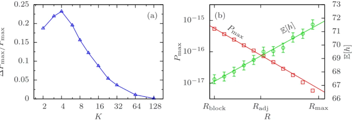
Figure 2.3. (a) Standard deviation ∆PmaxofPmaxwith random interactions for fixedL= 128 and varying K. Lines are for visual guidance. (b) Dependence of Pmax and E[h] on the rank R for fixedL = 128 and K = 8. Interaction schemes with certain rank are created with help of the algorithm described in appendix A.2.1. Each point corresponds to the average over 100 realizations. Lines are linear regressions.
fluctuations decline when K is of the same order as L, but they are quite significant when K is small. Interestingly, they are maximal for a value slightly above K = 2, resulting in non-monotonic behavior. Note, however, that the fluctuations are still very small compared to the difference between the averaged P
maxfor random interactions and P
maxfor adjacent interactions. It would be nice to study the fluctuations of E [h] as well, but they are hard to obtain since fluctuations caused by the integration algorithm are much larger than fluctuations due to the interaction scheme in that case.
Obviously, there are significant differences between the three classic interaction schemes in terms of P
maxand E [h]. What about interaction schemes that are not classic?
At this point it turns out that the rank R is a powerful tool for the quantification of arbitrary schemes [36, 37]. The dependence of P
maxand E [h] on R for fixed L and K is shown in figure 2.3(b). Although two schemes with the same rank might still have different properties, there is a rather clear correlation between these quantities and R. The (averaged) probability P
maxdecays roughly exponentially with R while E [h] increases linearly. When R is increased, the landscape properties seem to change smoothly from block model to the random model.
Exactly Solvable Example of Adjacent Interactions
In the following, the example of a Gamma distribution with shape parameter 1/2, K = 2, and adjacent interactions will be presented. The result for P
maxwas previously obtained in [37]. A gamma distribution with shape parameter 1/2 has a PDF given by
f (x) =
(
exp(−x)√πx
![Figure 2.2. Study of P max and E [h] on the NK landscape for fixed K = 8 (panel (a) and (c)) and fixed L = 128 (panel (b) and (d)), respectively](https://thumb-eu.123doks.com/thumbv2/1library_info/3705633.1506165/26.892.182.796.132.549/figure-study-landscape-fixed-panel-fixed-panel-respectively.webp)
![Figure 3.2. Probability P [X L > 0] of having at least one accessible path in a regular tree](https://thumb-eu.123doks.com/thumbv2/1library_info/3705633.1506165/37.892.121.677.134.467/figure-probability-p-having-accessible-path-regular-tree.webp)
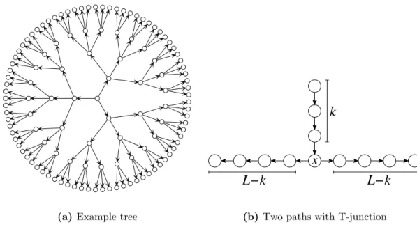
![Figure 3.4. Construction to improve the lower bound of P [X L,α > 0]. See the text for more details.](https://thumb-eu.123doks.com/thumbv2/1library_info/3705633.1506165/44.892.306.681.128.349/figure-construction-improve-lower-bound-p-text-details.webp)
![Figure 3.5. Probability P [X > 0] to have accessible paths on an n = 4 tree in dependence on the slope s of the RMF model with Gumbel distributed random part](https://thumb-eu.123doks.com/thumbv2/1library_info/3705633.1506165/52.892.326.640.136.364/figure-probability-accessible-paths-dependence-gumbel-distributed-random.webp)
