Fitness Landscapes, Adaptation and Sex on the Hypercube

(1)

Fitness Landscapes, Adaptation and Sex on the Hypercube

Inauguraldissertation zur Erlangung des Doktorgrades der Mathematisch-Naturwissenschaftlichen Fakult¨at

der Universit¨at zu K¨oln Vorgelegt von

Johannes Neidhart

aus Bergisch Gladbach

(2)

Universit¨at zu K¨oln Prof. Dr. Anton Bovier,

Rheinische Friedrich-Wilhelms-Universit¨at Bonn

Tag der m¨undlichen Pr¨ufung: 26.11.2014

(3)

I

Zusammenfassung

Diese Arbeit beschäftigt sich mit der theoretischen Betrachtung von Fitness- Landschaften im Kontext evolutionärer Prozesse. Diese verknüpfen das Genom eines Organismus mit seiner Fitness; sie sind ein wichtiges Werkzeug der theoretischen Evolutionsbiologie und seit wenigen Jahren auch im Blick- punkt experimenteller Studien. Im Folgenden werden Modelle von Fitness- Landschaften mit analytischen und numerischen Mitteln untersucht, mit der Zielsetzung, charakteristische Eigenschaften zu identifizieren, welche eine Zuordnung experimentell erschlossener Systeme ermöglichen. Desweiteren werden verschiedene adaptive Prozesse betrachtet; zum einen jene, welche mit Mutationen unter Selektion ablaufen, insbesondere sogenannte ‘Adaptive Walks’. Zum anderen auch solche, bei denen Rekombination hinzukommt, was die Komplexität der verwendeten Modelle erheblich steigert. Vor allem die entstehende Nichtlinearität der Zeitentwicklung erschwert die analytische Betrachtung, weswegen hier verstärkt auf Computersimulationen zurückgegriffen wird.

Abstract

The focus of this thesis is on the theoretical treatment of fitness landscapes in the context of evolutionary processes. Fitness landscapes connect an organism’s genome to its fitness. They are an important tool of theoretical evolutionary biology and in the recent years also experimental results became available. In this thesis, several models of fitness landscapes are analyzed with different analytical and numerical methods. The goal is to identify characteristics in order to compare the model landscapes to experimental measurements. Furthermore, different adaptive processes are examined. On the one hand such which run with mutations under selection, especially adaptive walks. On the other hand such which include recombination. Since these are non-linear in time development, an analytical approach is hindered which leads to an increasing use of computer simulations.

(4)

(5)

Chapter 1 Introduction

In the recent years the number of physicists working on problems from evolutionary biology grew steadily. Methods from theoretical physics can be applied, analogies found and models built.

This chapter shall give a brief introduction into the field and the used mathematics. Also the connection to theoretical physics will be made by the discussion of spin glasses. In ch. 2 the Rough Mt. Fuji model will be analyzed and certain properties will be calculated which lead to a suggestion of parameters to fit the model to experimental data. In this way it shall help to answer the question, which characteristics do such fitness landscapes have, and how can one tell if they are realistic? To extend this, Ch. 3 will present a way to reduce the number of data points to make statements about fitness landscapes of a certain family. This results in an algorithm which can also help to answer, how models can be fitted to experimental data. After these chapters about static landscapes, it will be asked, how does adaptation behave in certain evolutionary scenarios? Therefore dynamics are introduced and ch. 4 shall contain several analytic and numeric results on adaptive walks, amongst others a phase transition concerning the adaptive walk length in a Rough Mt. Fuji model. Finally, ch. 5 concerns the question: Why is sex?

Sexual reproduction and genetic recombination will be discussed and various results presented, most notable perhaps on the transient benefit of sex. A list of some of the used symbols and probability distributions in the appendix (app. A) shall avoid confusion. For completeness, the used algorithms that are not presented in the main text are described in app. B.

Throughout this thesis, the style is chosen to be a mixture of “classical”

mathematics literature and “modern” physics literature. This means, that important definitions and analytical results will be given separately with a reference number, and will be connected by running text. Results will usually be followed by a proof. Numerical results will not be stated in

1

(10)

this way but in the form of prose and figures, as these can usually not be formulated as exact and closed and need a description. The intention of this mixed presentation is to simplify reading and mark important passages in the inherent way of mathematical texts without exaggerated rigor. This means, that also calculations and intermediate results will be stated as proofs and results, which might not deserve the name from a mathematicians point of view. Nevertheless this drawback is accepted for the benefit of more clarity.

1.1 Biological foundation &

mathematical description

When an organism proliferates, it gives hereditary information to its offspring. This information is coded into its genome into a molecule which is called Deoxyribonucleic acid (DNA). This molecule is arranged in such a way, that the information is written in an alphabet of four bases, guanine (G), adenine (A), thymine (T) and cytosine (C), and all is shaped in a double helix, where bases are paired, G always with C and A always with T. This information will be copied into every cell of the developing offspring, as it was in the parent organism. A helpful metaphor gives Dawkins:

It is as though, in every room of a gigantic building, there was a book-case containing the architect’s plans for the entire building. The

‘book-case’ in a cell is called the nucleus. The architect’s plans run to 46 ‘volumes’ in a man – the number is different in other species.

The ‘volumes’ are called chromosomes. They are visible under a microscope as long threads, and the genes are strung out along them in order. It is not easy, indeed it may not even be meaningful, to decide where one gene ends and the next one begins. [. . .] ‘Page’ will provisionally be used interchangeable with gene, although the division between genes is less clear cut than the division between the pages of a book. [. . .] Incidentally, there is of course no ‘architect’. The DNA instructions have been assembled by natural selection. Dawkins [2, p.

22].

In a simplified picture where all genomes are assumed to be of the same length and also only haploid organisms are present, the genome is written with an alphabet A of four letters: A = {A, C, G, T}. The genetic information can be written as a sequence σ= (. . . , A, T, C, T, G, . . .). All possible sequences form thesequence space. Every position ofσ is calledlocus, and all elements of A which can be present at a locus are called alleles. Each realization σ is called a genotype. Usually, minor changes to the genome, like a change at

(11)

1.1. BIOLOGICAL FOUNDATION &MATHEMATICAL DESCRIPTION3

0000 0001

0010

0100

0011 0111

0101 0110

1000

1001 1010

1100

1011 1111

1101 1110

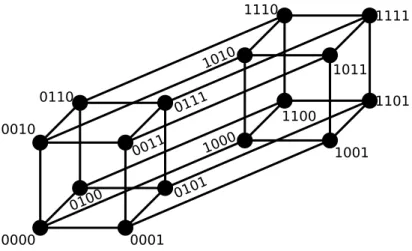
Figure 1.1: The binary sequence space is a hypercube of dimensionL. Here, the projection of a binary hypercube of dimension L = 4 is shown with the binary alphabet A={0,1}. [3]

a single locus, do not have a large effect on the organism. Thus, within a species, there are many genomes, which are different, but yield an organism of a certain species. If the organism proliferates sexually, a subset of individuals which can reproduce by mating is called a deme.

Of course, with a different alphabet A, also different systems can be described, for example RNA has the same structure and alphabet size, but different letters, proteins have a larger alphabet with 20 letters, each corresponding to an amino acid. For the study of theoretical models it is convenient to restrict to a binary alphabet A = {+1,−1} =: B. Although this results in a lack of generality, and a generalization is often hard, it enables the use of a many different analytical and numerical methods. And although the reduction of biological information seems drastic, the binary system can still be interpreted in a variety of biological ways, for example the presence or absence of a gene, the state (active or passive) of a gene, or the absence or presence of a mutation. Also, it is very close to the physical systems of spin glasses. Following this tradition, this work is done usingB, if not mentioned otherwise.

In the binary alphabet, all sequences of a fixed length L span the L–

dimensional hypercube H^L as sequence space, see fig. 1.1. H^L is a metric space equipped with the Hamming distance:

Definition 1.1. The Hamming distance is a metric on the hypercube. It is

(12)

defined as

d:H^L×H^L → {0,1, . . . , L} (σ, σ^′)7→

L

X

i=1

1−δ_σ_i_,σ^′_i

with the Kronecker Delta δ. This implies that the maximal Hamming distance between two sequences σ, σ^′ is d(σ, σ^′) = L. If d(σ, σ^′) = L, σ^′ is also called the antipodal of σ and will be labeled σ.

H^L consists of 2^L sequences. Each sequence σ has L neighbors σ^′ with d(σ, σ^′) = 1 and in general the number of sequences at Hamming distance d is ^L_d

(see (A.4) for the convention on binomial coefficients). Thus, with respect to a given σ ∈ H^L most other σ^′ ∈ H^L lie at Hamming distance d(σ, σ^′) = ^L₂, where ^L_d

d=L/2 = _(L/2)!^L! is maximal. In graph theoretical notion,H^L is a regular graph (because every sequence has the same amount of neighbors), with 2^L vertices (neighbors) and 2^L⁻¹L edges (connections between neighbors). The information about the structure of H^L is also contained in the adjacency matrix of H^L.

Definition 1.2. The adjacency matrix A is a 2^L×2^L matrix, defined by Aσ,σ^′ =

(1, d(σ, σ^′) = 1

0, else. (1.1)

1.2 The struggle for existence

The severe and often-recurrent struggle for existence will determine that those variations, however slight, which are favorable shall be preserved or selected, and those which are unfavorable shall be destroyed. This preservation, during the battle for life, of varieties which possess any advantage in structure, constitution, or instinct, I have called Natural Selection; and Mr. Herbert Spencer has well expressed the same idea by the Survival of the Fittest. Darwin [4]

“The Survival of the Fittest” is perhaps the most popular phrase connected to evolutionary biology. Although evolutionary biologists meanwhile refrain to use it due to its lack of generality and high potential for misunderstanding, the impact is remarkable. It has been used in and inspired works on early theories of evolution [5], economy, sociology and politics [6]. And still, in hindsight, set in the correct context it gives a very

(13)

1.2. THE STRUGGLE FOR EXISTENCE 5 nice description of evolutionary processes of many kinds, formulated in a time when the molecular basis of evolution was not even set.

Nevertheless, the phrase was not only misunderstood often but was also abused. The word ‘fittest’ can be interpreted in terms of physical or economical strength and toughness, which lead to the attempt to build a biological foundation and justification of the suppression of the weaker [6]. The real meaning of fitness in the biological context is probably ‘best adapted’. The confusion about the term fitness is nevertheless, it seems, not only a problem outside evolutionary biology, but also for scientists in the field [7]. Therefore, this section is intended to clarify the used terms, introduce the mathematical language used to analyze evolutionary processes and give a few basic results.

There are at least two commonly used definitions of the term fitness on a molecular level.

Definition 1.3. If n(σ, t) individuals carry the genotype σ at time t the Malthusian fitness F(σ) is defined by

d

dtn(σ, t) = F(σ, t)n(σ, t). (1.2) Hence, F(σ) is the growth rate of the organisms with genotype σ in continuous time.

Definition 1.4. Based on the last definition, the Wrightian fitness w(σ) is defined by solving the differential equation (1.2) defining the Malthusian fitness:

n(σ, t+ 1) =w(σ, t)n(σ, t) (1.3) which implies the relation w(σ, t) = e^R⁰^t^F^(σ,t^′^)dt^′ , or for time independent fitnessw(σ) = e^F^(σ). This fitness definition is particularly useful in a discrete time scenario, where the generation time t_g is set 1 for convenience. In the following, if not mentioned otherwise, time independent fitness is of interest.

Although mostly F will be used to denote fitness, concerning the properties of fitness landscapes the results do also apply to the Wrightian fitness w. Nevertheless, if using w it has to be ensured that for all σ ∈ H^L : w(σ) ≥ 0, which is not necessary for the Malthusian fitness F. Usually fitness is seen as a measure for reproductive success and thus the above definitions are very common. Nevertheless, in experiments it might be more convenient to measure a proxy for fitness. This might be for example the output of a certain protein [8] or the resistance to an antibiotic [9].

Defining fitness in dependence of the genotype, it is natural to think of F as a mapping from the sequence space into the real numbers.

(14)

Definition 1.5. A fitness landscape is a mapping F :H^L →R

σ 7→F(σ). (1.4)

The idea of a fitness landscape was according to McCoy [10] first presented by Toulon in 1895 who used a different name. Nevertheless mostly Wright is credited and he also introduced the notion ‘fitness landscape’

[11]. Before experimental data became available in the recent years (see e.g. [12] for a review), the study of fitness landscapes was purely theoretical.

Early population geneticists often used additive fitness landscapes for their mathematical analysis.

Definition 1.6. The Mt. Fuji landscape is an additive fitness landscape.

Given an arbitrary reference sequence σ^∗, the fitness is distributed as Fσ^∗(σ) =−cd(σ, σ^∗).

Additive means here, that all loci are independent from each other, and the change in fitness resulting from the change of one locus never depends on the rest of the genome, which is also called the genetic background. An additive landscape only has one global fitness maximum: a point in the landscape at which all neighbors have lower fitness. Perhaps the most prominent arguments about the biological legitimacy of additive fitness landscapes is ‘the beanbag genetics dispute’ between the two friends Mayr and Haldane. While Haldane favored the simplicity of the additive model due to the mathematical possibilities, Mayr rejected it, calling genetics on such a model ‘beanbag genetics’ [13].

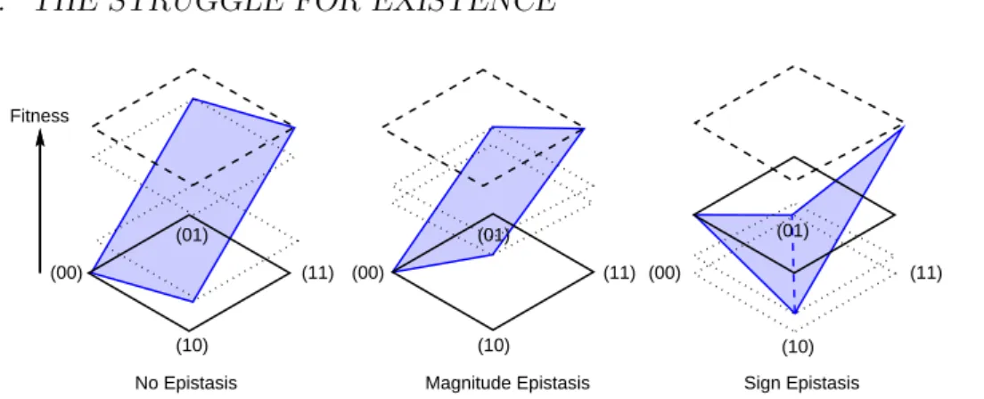
Opposed to the additive landscapes are theepistaticlandscapes. Epistasis means nothing but the absence of additivity. One distinguishes basically two types. One is magnitude epistasis, where a beneficial (deleterious) mutation will be beneficial (deleterious), regardless of the genetic background, but its impact may vary. The other issign epistasis [14] which means that not only the magnitude of the effect of a mutation may vary, but also its sign, thus a formerly beneficial mutation may become deleterious, depending on the genetic background. While additive and magnitude epistatic landscapes can only have one global fitness maximum, sign epistasis enables the possibility of multiple fitness maxima, see fig. 1.2. Due to this property, landscapes with a lot of sign epistasis are also calledrugged. A model for such a rugged landscape was introduced by Kingman [15] as follows:

Definition 1.7. If all fitness values F(σ) are identically and independently distributed (i.i.d.) random variables, F is called House-of-Cards (HoC) landscape.

(15)

1.2. THE STRUGGLE FOR EXISTENCE 7

(10) Fitness

(00)

(10) (01)

No Epistasis

(11) (00)

(01)

(10)

(11)

Magnitude Epistasis (00)

(01)

(11)

Sign Epistasis

Figure 1.2: Illustration of the different types of epistasis in a two dimensional hypercube with alphabetA={0,1}. Only in the case with sign epistasis multiple fitness maxima are possible.

The HoC- and the Mt. Fuji-model describe in some sense contrary extremes of fitness landscapes. Although the HoC-landscape is more complex due to the high degree of epistatic interactions, it is still mathematically well feasible. A natural generalization is an interpolation between these two landscapes.

Definition 1.8. Let σ^∗ ∈ H^L be an arbitrary reference sequence, and let {ξi}be a set of 2^L i.i.d. random variables. Then with c∈R

Fc,σ^∗(σ) =−cd(σ, σ^∗) +ξσ

is called the Rough-Mt.-Fuji (RMF) landscape [16, 17, 18]. Note that for c → ∞ and c → 0 the Mt. Fuji and the HoC-landscapes are retrieved, respectively.

Definition 1.9. An alternative definition is given as follows. Let σ^∗ ∈ H^L be an arbitrary reference sequence, and let {ξi} be a set of 2^L i.i.d. random variables. Then withc∈R

Fc,σ^∗(σ) =cd(σ, σ^∗) +ξσ

is also called the Rough-Mt.-Fuji (RMF) landscape

Note that both definitions of the RMF-model are equivalent in the sense, that by a simultaneous change c → −c and d → L − d both can be transformed into one another.

The RMF-model provides the possibility to tune the correlations in the landscape. It is a more flexible model than the HoC which results in a more complicated mathematical analysis as trade-off.

(16)

Another popular model for fitness landscapes with epistasis is Kauffman’s LK-model [19]¹. The idea is that each locus interacts withK other loci. The subsequence containing a locus and the loci it interacts with is called itsLK- neighborhood. Since anLK-neighborhood has the sizeK+ 1, it is convenient to introducek =K+ 1.

Definition 1.10. Let {fi : B^k → R} be a set of i.i.d. random functions and let{Ξ(σi)} be a set of LK-neighborhoods (Ξi ∈B^k). The LK-model is defined by the fitness function

F(σ) = 1

√L

L

X

i=1

fi(Ξ(σi)).

Often used choices for LK-neighborhoods are for example the adjacent neighborhood Ξ(σi) = (σi, σi+1, σi+2, . . . , σi+K), or the random neighborhood, where besides σ_i all K other loci are chosen at random. Note, that simple generalizations of the LK-model are achieved by altering the LK- neighborhoods to vary in size or to exclude σi.

TheLK-model is, as the RMF-model, suited to tune between the Mt.-Fuji landscape (k = 1) and the HoC-landscape (k = L) [19, 20, 21, 22, 23, 24], although thek values in between do not yield a ‘smooth’ transition as in the RMF-landscape.

For convenience a fitness landscape with a random component which is distributed according to a distribution function P will be called P- distributed.

1.3 Evolutionary processes

The definitions of fitness 1.3 and 1.4 already imply an evolutionary process of selection which is one of the three evolutionary forces:

Definition 1.11. The three evolutionary forces are the mechanisms associated to the three parameters s (selection coefficient), N (population size) and µ(mutation rate).

• Selection ∼ s is a relative fitness measure which leads to focusing around particularly fit sequences. Its timescale is τs∝ ¹_s.

1Kauffman called the modelN K, referring to the sequence length asN, but because it is more common to call the population sizeN, the model is re-labeled here.

(17)

1.3. EVOLUTIONARY PROCESSES 9

• Genetic drift ∼ _N¹ is caused by demographic stochasticity, fluctuations in the number of offspring. Its timescale is τN ∝N.

• Mutation ∼µleads to stochastic changes in the genome, the timescale is τ_µ∝ _µ¹.

Note that mutation and genetic drift introduce two different types of stochasticity.

Point mutations occur with probability µ. A point mutation is a randomly occurring change of allele at one locus, more precisely given two neighboring sequences σ, σ^′ ∈ H^L = B^L a point mutation σ → σ^′ at the ith locus is a transition σi → −σi, comparable to a spin-flip in physics. If only two neighboring sequences are available and the mutation rate is the same in both directions, the following Langevin-equation is an extension of def. 1.3 and describes the evolution of n(σ, t) under mutation, selection and reproductive fluctuations. In the situation where two genotypes σ, σ^′ with d(σ, σ^′) = 1 are present and thus n(σ^′, t) =N −n(σ, t), it reads

d

dtn(σ, t) = F(σ, t)n(σ, t) +χ(σ, t) +µ(N −2n(σ, t)), (1.5) with a random variable χ with hχ(σ)i= 0 and hχ(σ, t), χ(σ, t^′)i =δ(t−t^′).

It can be transformed into a Fokker-Planck-equation by Kramers-Moyale expansion [25], see e.g. [26] for the calculation. In population dynamics this is calledKimura equation. Thefrequency ofσ is defined byp(σ) = ^n(σ)_N . The Kimura equation gives the change of the probability that a sequence σ has frequencyp at time t [27, 28]:

∂

∂tP(p, t) = 1 2N

∂²

∂p²p(1−p)P(p, t) (1.6)

−(F(σ, t)−F(σ^′, t)) ∂

∂pp(1−p)P(p, t) +µ ∂

∂p(1−2p)P(p, t).

In this context, the drift term is composed of mutation and selection, while the diffusion term is called genetic drift. Note, that in the presence of only two sequencesn(σ) +n(σ^′) =N and thusp(σ) +p(σ^′) = 1. The probability, that all individuals will carry only one of the two sequences is called fixation probability and was calculated by Kimura [29] to be

u(σ, σ^′) = 1−e⁻^2(F^(σ^′⁾⁻^F^(σ)) 1−e⁻^2N(F^(σ^′⁾⁻^F^(σ)) ≈

(0, F(σ^′)−F(σ)<0 1−e⁻^2(F^(σ^′⁾⁻^F(σ)), F(σ^′)−F(σ)>0

(1.7)

(18)

where the approximation holds if N|F(σ^′)−F(σ)| ≫1.

If more than two sequences are available, it is convenient to write the evolutionary equations as a matrix equation.

Definition 1.12. Theselection matrix S is defined bySσσ^′ =w(σ)δσσ^′. The mutation matrix Mis defined byM^σσ^′ = (1−µ)δσσ^′+^µ_LAσσ^′. To formulate matrix equations it is necessary to understand n, p and w as vectors which contain as elements n(σ), p(σ) and w(σ) respectively.

The mutation-selection equations in a discrete time setting are then

n^t+1 =SMn^t unnormalized

p^t+1 = SMp^t P

σ∈H^L(SMp^t) (σ) normalized (1.8) where the time t is measured in generations.

1.4 Evolutionary regimes

A common way to start the analysis of population genetic problems is to classify the problem according to itsevolutionary regime, which is determined by the relative size of the evolutionary parameters

• N µ <1 is theweak mutation regime: on average not every generation a new mutant arises.

• N µ > 1 is the strong mutation regime: on average every generation more than one new mutant arises. This can lead to a very diverse population.

• |N s| ≪ 1 is the weak selection regime: the fixation probability is low and a diverse population is probable.

• |N s| ≫ 1 is the strong selection regime: beneficial mutants are very likely to fix, while deleterious mutants will probably go extinct very fast.

A combination of those regimes which is of particular interest in this thesis is the Strong-Selection-Weak-Mutation regime (SSWM) first introduced by Gillespie [30]. As the name indicates, selection is strong (|N s| ≫ 1) while only few mutations arise (N µ≪1). This leads to a situation, where double mutations are impossible in the sense, that selection either fixes beneficial mutations or kills individuals with deleterious mutations before a double

(19)

1.5. RECOMBINATION 11 mutation arises. Thus, the population is monomorphic, i.e. all individuals have the same genome, all the time except for the short period of time when a new mutant was created and is evaluated by selection. This means, that besides the definition of the regime, mutation rate and population size do not affect the dynamics because the fixation probability is approximated by (1.7).

The resulting evolutionary process is called adaptive walk, the population can be seen as a walker on the hypercube which can only make steps to neighboring sequences with a higher fitness. This implies, that the walker must stop as soon as a localfitness maximum is reached, which is defined by the absence of fitter neighbors. There are different kinds of adaptive walks, which differ in the transition probability to the next sequence. It is common to distinguish between three different processes:

Greedy adaptive walks (GAW): The next step is always taken to the fittest sequence in the neighborhood.

Random adaptive walks (RAW): The next sequence is chosen at random from the sequences of the neighborhood which are fitter than the current one.

Natural adaptive walks (NAW): The next sequence is chosen from the neighborhood with a probability proportional to the fitness difference

Pσi→σj = (F(σj)−F(σi))Θ(F(σj)−F(σi)) PL

k=1(F(σk)−F(σi))Θ(F(σk)−F(σi)). (1.9) This transition probability was derived from (1.7) by Gillespie [31].

Since all three processes are restricted to increase fitness in every step they will, for finite L, eventually stop after a finite number of steps. The mean walk lengthℓ is the mean number of steps until a local optimum is reached, where the average is taken over runs and landscapes. ℓ is one of the most important properties of adaptive walks.

If a sequence σ^′ can be reached by an adaptive walk which started on another sequence σ, a path must exist from σ to σ^′ in which the fitness increases in every step. If such a path exist, it is called accessible.

1.5 Recombination

A reproduction strategy which is very common in nature isrecombination. It leads to the genetic variation by introduction of (parts of) a second genome which is intertwined with the first one. This can for example happen by

(20)

sexual recombination, where the genome of two parents is recombined, but also by transformation, a process in which certain kinds of bacteria take up and incorporate exogenous genetic material. The success of recombination, especially sex, is one of the great mysteries of modern science. Although its apparent superiority in large parts of nature, it is not understoodwhy sexual reproduction can be of benefit at all. Very simple economic reasoning gives rise to questions, e.g. the fact, that two parents are needed to reproduce without increasing the number of offspring has become famous as the two- fold cost of sex [32, 33]. But also without the costs, it is not clear whether recombination gives any benefit at all [34, 35, 36, 37], one point being, that recombination might break apart useful structures in the genome, which is known as recombination load [38].

Nevertheless, this paradox has inspired several attempts to explain the prevalence of recombination:

Muller’s ratchet & deterministic mutation hypothesis: recombination enables a population to purge deleterious mutations [39, 40, 41] faster than asexuals, which have to wait for a back-mutation.

Fisher-Muller- & Hill-Robertson-effect: If two beneficial mutations occur in a population, both can spread fast, without the need of two double mutations [42, 43, 44, 40].

Weismann effect: More variation is created [45].

Fisher’s fundamental theorem: Here, the benefit follows from the Weismann effect, stating that the mean fitness increase is proportional to the genetic variance [42]. Sadly, this result is not generally true but assumes the absence of epistasis [46], or it needs a certain kind of variance measure [47].

Red Queen Hypothesis: Recombination increases the speed of adaptation, not necessarily the ultimate fitness. This way, organisms can adapt quicker to the surroundings than other ever-evolving species [48].

The mathematical description of recombination will be done in a similar manner as mutation above, following Stadler and Wagner [49]. And as before, the sequence length is constrained to be constant.

Definition 1.13. The recombination operator R is a mapping into the powerset ofH^L:

R:H^L×H^L →P(H^L)

(σ, σ^′)7→{σ^′′|σ^′′i =σi∨σ^′′i =σ^′_i}.

(21)

1.6. EXTREMES: FITNESS AND PROBABILITY 13 R(σ, σ^′) is the set containing all possible recombinations of σ and σ^′ which have the same lengthL.

The adjacency matrix is not the matrix containing the most valuable information about the structure of the process anymore, as it was for mutation. It is replaced:

Definition 1.14. The incidence matrix H is to recombination what the adjacency matrix is for mutation. It is defined by

Hσ,(σ^′,σ^′′) =

(1, σ ∈R(σ^′, σ^′′) 0, else.

In terms of H, a recombinatorial transition matrix can be defined by Tσ^′→σ = X

σ^′′∈H^L

p(σ^′′)p(σ^′) Hσ,(σ^′,σ^′′)

|R(σ^′, σ^′′)|. There, | • |means the cardinality.

In the definition of T it becomes obvious, that recombination is quadratic in the population frequency p and not, as mutation, linear.

There, recombination is incorporated by using a uniform crossover, i.e. the recombined sequence is put together in such a way, that at each locus the allele is taken from one of the corresponding parent genomes at random.

Other possible crossovers are, e.g., single point crossover, where the parent genomes are cut at a certain point and the fronts and rears are exchanged. Or thetwo-point-crossover where the genomes are cut two times and the middle part is exchanged. At such a crossover two possible genomes are created of which one has to be chosen at random. In the following, only the uniform crossover will be analyzed.

1.6 Extremes: Fitness and probability

In ‘everyday statistics’ it is important to understand theaverage behavior of apparently random events. One of the most used tools to do so is thecentral limit theorem. Its statement is the following:

For every set of n i.i.d. random variables {Xi} with expected value µ and varianceσ², the random variable√

n(Pn

i=1Xi−µ) converges in distribution to a Normal-distribution, more precisely

√n 1 n

n

X

i=1

Xi−µ

!

−d

→ N(0,Var(Xi)) (n → ∞). (1.10)

(22)

As mentioned above, the central limit theorem describes the average behavior, which is reflected by the fact, that it is a statement about asum of random variables. Now, in some cases the average is not of particular interest.

For example is an average tide nothing to worry about. But what is of critical interest is the height ofextreme tides. If a city builds a levee, it has to know that it is high enough to withstand not only the everyday flood, but also the one-in-a-century flood. In evolutionary biology the extremes are important, too. The sequence space is so large, that probably most of the possible genomes are lethal. Only extraordinary fit sequences bear the possibility to be viable. Instead of the average behavior, it is now important to describe the maxima and the extraordinary large of a set of random variables. In the last century this part of mathematics has become very successful under the name Extreme-Value-Theory (EVT).

Definition 1.15. The Generalized-Extreme-Value-Distribution (GED) is defined by the distribution function

G(x;µ, σ, κ) = exp (

−

1 +κ

x−µ σ

₋1/κ) .

It has a scale parameterσ, a location parameterµand a shape parameter κ with the restriction 1 +κ(x−µ)/σ >0.

Theorem 1 (Fisher-Tippett-Gnedenko [50, 51]). Let {X_i} be a set of n i.i.d. random variables and Mn = max(X1, . . . , Xn). Suppose there exists a sequence of constants an>0, bn with

P

M_n−b_n an ≤x

→D(x) (n → ∞)

with a non-degenerate distribution function D, then parameters can be found such that D(x) = G(x;µ, σ, κ).

The shape parameter κ governs the tail behavior of the GED. In terms of κthree probability classes can be defined, each containing the probability distributions which converge to a corresponding GED in terms of thm. 1:

• κ = 0: Defines the Gumbel class or type I distributions. This class contains distributions with a tail vanishing faster than power law.

• κ > 0: Defines the Fr´echet class or type II distributions. This class contains all distributions with power law tail.

(23)

1.6. EXTREMES: FITNESS AND PROBABILITY 15

• κ < 0: Defines the Weibull class or type III distributions. GED has a support limited to the right by µ− ^σ_κ. This class contains all distributions with power law tail and bounded support.

Another approach to the analysis of extreme values is via Peaks-Over- Threshold (POT). If P is some distribution function and u is a threshold, theexcess function is the distribution function for valuesover the threshold:

Eu(y) =P(X−u≤y|X > u) = P(u+y)−P(u) 1−P(u) .

Definition 1.16. TheGeneralized-Pareto-Distribution (GPD) is defined by the distribution function

GPD(κ,µ,σ)(x) =





 1−

1 + ^κ(x_σ⁻^µ)−1/κ

for κ6= 0, 1−exp −^x⁻_σ^µ

for κ= 0,

for x > µ when κ > 0, and µ 6 x6 µ−σ/κ when κ < 0, where κ has the same role as in the GED and gives the same information about the extreme value class. µ and σ are location and scale parameter, respectively.

Theorem 2 (Pickands-Balkema-deHaan [52, 53]). Let {Xi} be a set of n i.i.d. random variables. Then parameters can be found, such that:

E^u(y)→GPD(κ,µ,σ)(y) (u→ ∞).

Although both approaches have been proved to be very powerful in the past, usually for data analysis the limits n → ∞ or u → ∞ cannot be satisfied. Thus, as an alternative to the above discussed ultimate EVT, the penultimate EVT deals with the description of large but finite sets of i.i.d. random variables. It might in such a case be better to describe a given dataset with a distribution function which has a different κthan its limiting distribution function. Assuming, that a set{Xi}of ni.i.d. random variables with distribution functionP which has a limiting distribution withκ= 0 (one says it is in the domain of attraction of Gumbel type). Then the (1− _n¹)th quantile q(n) = P⁻¹(1−_n¹) is an approximation for the typical largest value.

The hazard function is defined by h(x) =

d dxP(x)

1−P(x). (1.11)

It has only a finite limiting value limx→∞h(x) for distributions with exponential tail. One choice of the shape parameter is then [54]

κn= d dx

1 h(x)

x=q(n)

. (1.12)

(24)

The fact that even distributions from the Gumbel class might behave like non- Gumbel-class distributions for finite sample sizes emphasizes one thing: it is always important to know how things are for distributions besides the domain of attraction of Gumbel type. All experimental data sets are finite, which implies the necessity to investigate the behavior of processes, correlations, etc. for all three probability classes.

1.7 Spin glasses & other fields of interest

Spin glasses (also called amorphous magnets) are magnetic substances in which the interaction among the spins is sometimes ferromagnetic (it tends to align the spins;J_ik>0), sometimes antiferromagnetic (it antialigns the spins;J_ik<0). The sign of the interaction is supposed to be random. In some spin glasses the spins can take only two values

±1 (Ising spins) [. . . ]. Mezard et al. [55]

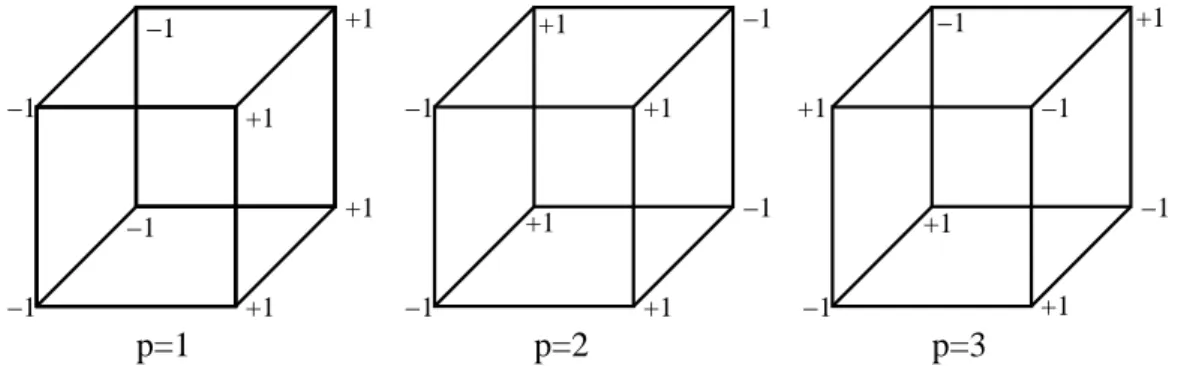
In the above quote,Jik are the couplings, or interactions, between two spinsi andk. Their supposed randomness leads to inherentdisorder, more precisely quenched disorder. Considering spin glasses of Ising spins means that spin configurations σ are elements from the hypercube H^L, and also, that H^L is the configuration space for this spin glass model. The spatial configuration of the spins (chain, lattice, etc.) enters through the interactions. The energy of each configuration is measured with help of theHamiltonian H(σ) which corresponds to negative fitness. Special states in the system are those which minimize energy. Those are called (meta)stable states. This means, that the Hamiltonian corresponds to a negative fitness landscape in the picture of evolutionary biology where fitness maxima are (meta)stable. A stable state or ground state corresponds to a global fitness maximum, whereas a metastable state corresponds to a local fitness maximum. If a fitness landscape shows sign epistatis, the corresponding situation in spin glass analysis is called frustration. Both fields are in fact very similar. This is also expressed in the similarity of models. A toy model which was proposed by Derrida [56] is theRandom Energy Model (REM) in whichH(σ) are i.i.d. random variables.

This corresponds to the House-of-Cards model for fitness landscapes. As a straight forward generalization Derrida [57] proposed the p-spin-model [58], in which subsets ofpof theLspins are interacting and the Hamiltonian takes the form

H(σ) =− X

i1...ip

Ai1...ipσi1. . . σip

(25)

1.8. EXPERIMENTS AND FITNESS PROXIES 17 with random contributions Ai1...ip. This model is the analogue of the Fourier expansion of a fitness landscape (see sec. 3.2 for details). Each coefficient Ai1...ip introduces interactions between p spins. Since in the LK-model the number of interacting loci is determined by K it can be understood as a superposition of sparse p-spin-models since in general many coefficients are null. The RMF-model corresponds to a REM model in an external magnetic field, which has the Hamiltonian

H(σ) = aξσ −µ

L

X

i=1

hσi

with amagnetic moment µ, fieldhand a constantawhich ensures the correct dimension.

Adaptive processes are linked to spin glasses as well. For example are adaptive walks very similar to a Metropolis dynamics on a spin glass at zero temperature [59]. The relaxation dynamics of a spin glass in an exterior magnetic field have been studied in the context of spin-glassaging [60], which is related to adaptive walks on an RMF-landscape.

Spin glasses are nevertheless not the only area, where similar models apply. Basically in all fields, in which binary structures appear, similarities occur. A very prominent example for that are several problems in computer science (e.g. [61]).

The probability for the existence of accessible paths on fitness landscapes [24] is closely connected to percolation [62]. Recently, in the context of an RMF model on a Cayley tree (which is very similar to the hypercube for large L) the term accessibility percolation was coined [63].

1.8 Experiments and fitness proxies

Although the basic ideas of fitness and fitness landscapes are several decades old, the experimental tools for fitness measurements are quite new (or only recently technically available). There are basically two approaches in the experimental study of fitness landscapes [64].

For the first one, the evolution of organisms with a short generation time is observed and the fitness development is measured and compared to the ancestors (e.g. [65]). From the fitness changes, properties of the underlying landscape can be inferred on a qualitative level. Although the generated data sets may cover large regions of the genotype space, the resulting picture of the fitness landscape is incomplete. Additionally, it is biased by the evolutionary regime and the resulting adaptive dynamics.

(26)

Fitness values which are obtained in a similar way are compared to an RMF-landscape in sec. 2.3. The data from Miller et al. [66] are fitness values of the bacteriophage ID11. The measurements were performed in a bottleneck manner [67]: in several passages, the bacteriophage was allowed to grow in a bacterial host medium, here Escherichia coli C, for one hour.

Then the process was stopped and the growth rate measured to calculate the fitness.

The second approach relies on the analysis of predefined mutations, which are created to observe the fitness in a tiny, but complete part of the hypercube. For experimental convenience, it is common to not measure Malthusian or Wrightian fitness itself, but a proxy, such as antibiotic resistance.

In sec. 3.5 empirical landscapes of the second type are compared to model- landscapes. One “real” fitness landscape is the L = 6 landscape from Hall et al. [68] of yeast, fitness is measured as growth rate. Another one is theL= 8 growth rate landscape of the fungus Aspergillus niger presented by Franke et al. [69]. Additionally two L = 9 landscapes which measure the output of certain enzymes in Nicotiana Tobaccum as a fitness proxy, specifically the enzymatic specificity of terpene synthases, that is, the relative production of 5-epi-aristolochene and premnaspirodiene, presented by O’Maille et al. [8]

were analyzed. The last two landscapes are not complete, only 418 of the 512 fitness values are given. The missing data points are interpolated by fitting a linear model [70].

(27)

Chapter 2 The Rough-Mt.-Fuji model

In this chapter, several properties of the RMF-model (def. 1.8) will be calculated and it will be fitted to experimental data. It was introduced by Aita et al. [16] in the context of biopolymers in a slightly more general way. In the following, the calculations will be restricted to the def. 1.8 and the reasoning is close to [18].

2.1 Further remarks on the definition

The Rough Mt. Fuji Landscape will in this chapter be used as defined in def. 1.8. Because the mean fitness gradient is for c >0 directed towards σ^∗, RMF-landscapes are not isotropic. On average, fitness increases in one and decreases in another direction. These directions are defined by the change in Hamming distance to σ^∗, d(σ, σ^∗).

Definition 2.1. The neighborhood-set ν of a sequence is defined by

ν(σ) = {σ^′|d(σ, σ^′) = 1} ∪ {σ}. This set is split in three parts (d(σ, σ^∗) =:d):

• The uphill–neighborhood ν^↑(σ) = ν(σ)∩ {σ^′|d(σ^′, σ^∗) = d−1} which contains all neighbors which are closer toσ^∗ and thus have an average fitness advantage of c,

• σ itself in ν(σ)^• ={σ},

• and the downhill–neighborhood ν^↓(σ) = ν(σ)∩ {σ^′|d(σ^′, σ^∗) = d+ 1} which contains all neighbors which are further away from σ^∗ and thus have an average fitness disadvantage of c.

Obviouslyν(σ)^↑∪ν(σ)^•∪ν(σ)^↓ =ν(σ).

Note that the fitness values in the RMF-landscape are not i.i.d. but correlated random variables.

19

(28)

0.01 0.1

0 2 4 6 8 10

pcmax

d (a)

c=0.1 c=0.3 c=1 c=3

0 0.1 0.2 0.3 0.4 0.5 0.6 0.7 0.8 0.9 1

0 20 40 60 80 100

Prob. that the largest is up/down

d

(b) c=0.1

c=0.3 c=3

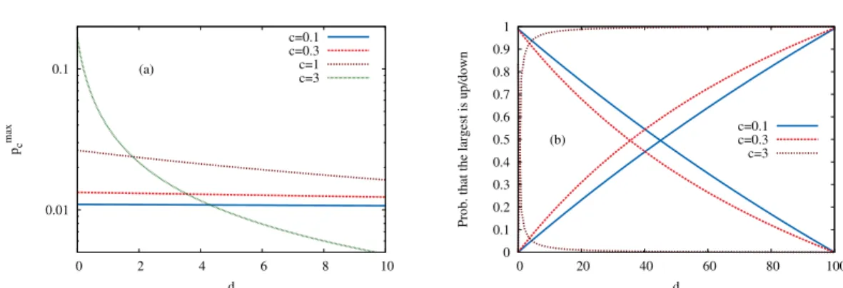
Figure 2.1: (a) The probability that a given sequence is a local fitness maximum is shown as a function of the distancedto the reference sequence for several values of c and L = 100. (b) The probability that the neighboring sequence of largest fitness is in the uphill (solid lines) or downhill (dashed lines) direction is shown as a function ofdfor different values of cand L= 100. Both plots show results of a Gumbel distributed RMF-landscape.

2.2 Fitness maxima & correlations

One of the characteristic properties of a fitness landscape is the number of fitness maxima. It gives information about the landscape’s roughness and is also a so called ‘epistasis measure’ [12]. In the HoC-landscape, the probability p^max, that F(σ) is a fitness maximum, is equal to the probability, that it is the largest fitness value in {F(σ^′)|σ^′ ∈ ν(σ)} which is _|_ν(σ)¹ _| = _L+1¹ . In the RMF-model the probability depends additionally on the parameters c and d as well as on the underlying probability distribution. If the distribution function of the random variables is P, the probability can be written as

p^max_c (d) = Z

dx p(x) (P(x−c))^d(P(x+c))^L⁻^d. (2.1) The sums in the argument of the distribution function prevent a general evaluation of the integral. A special case is theGumbel distribution P_G(x) = e⁻^e^−x. It is a limiting distribution in the Gumbel class,PG(x) = GEV0,1,0(x), which comes with a very usefulshifting property:

PG(x+c) =e⁻ê^−x−c =eê^−xê^−c =

e⁻^e^−x₋e^−c

=PG(x)⁻^e^−c (2.2) Result 2.1 (p^max_c in the Gumbel case). In the Gumbel case, the probability that a given sequence is a fitness maximum is given by

p^max_c (d) = 1

1 +de^c+ (L−d)e⁻^c.

(29)

2.2. FITNESS MAXIMA & CORRELATIONS 21 Proof. Using the shifting property on (2.1) yields:

p^max_c (d) = Z

dx p(x) (P(x−c))^d(P(x+c))^L⁻^d

= Z

dx p(x) P(x)⁻^e^cd

P(x)⁻^e^−cL−d

=

Z

dPG P_G⁻^e^c^d⁻^e^−c^(L⁻^d)= 1

1 +de^c + (L−d)e⁻^c.

The behavior of res. 2.1 for intermediate values of c is illustrated in fig. 2.1(a).

Besides the special case of the Gumbel distribution, it is possible to approximate (2.1) following [71, 72] by expanding in c:

p^max_c (d) = 1

L+ 1 +c(L−2d)I_L₋₁+O(c²) with I_L₋₁ = Z

dx p(x)²P(x)^L⁻¹. (2.3) Expressions forILfor representatives of the three extreme value classes have been derived by Franke et al. [71]. For large L the integral behaves as [72]

IL ∼L⁻^(2+κ), (2.4)

where κ denotes the extreme value index from def. 1.15. This implies a stronger effect of con the number of maxima for Weibull class distributions than for Fr´echet or Gumbel class distributions.

The anisotropy of the landscape also inspires the question, in which direction the fittest neighbor is positioned. Although the uphill neighbors have a fitness benefit of c, the number of neighbors in ν^↑ and ν^↓ varies with the position with respect to the reference sequence. The corresponding probabilities to find the fittest of the neighborhood uphill or downhill are p^↑_c(d) andp^↓_c(d). A modification of (2.1) restricted toν^↑(σ) andν^↓(σ) yields the general expressions

p^↑_c(d) =d Z

dx p(x)P(x)^d⁻¹P(x+c)P(x+ 2c)^L⁻^d, (2.5) p^↓_c(d) = (L−d)

Z

dx p(x)P(x)^L⁻^d⁻¹P(x−c)P(x−2c)^d, (2.6) which can be explicitly evaluated for the Gumbel distribution.

(30)

Result 2.2(Fittest is up/down in the Gumbel case). In the Gumbel case, the probability, that the fittest of the neighborhood is positioned uphill/downhill is given by

p^↑_c(d) = d

d+e⁻^c+e⁻^2c(L−d), p^↓_c(d) = L−d

L−d+e^c+e^2cd. Proof.

p^↑_c(d) = d Z

dx p(x)PG(x)^d⁻¹PG(x+c)PG(x+ 2c)^L⁻^d

= d

Z

dPG p(x)PG(x)^d⁻¹PG(x)⁻^e^−c(PG(x)⁻^e^−2c)^L⁻^d

= d

Z

dPG P_G^(d⁻^1)+e^−c^+e^−2c^(L⁻^d)

= d

d+e⁻^c+e⁻^2c(L−d) and analogously for p^↓_c.

Note that p^↑_c +p^↓_c +p^max_c = 1 and p^↑_c = de^cp^max_c , p^↓_c = (L−d)e⁻^cp^max_c . d induces a benefit to the largest sub-neighborhood which is ν^↑(σ) (ν^↓(σ)) if d < ^L₂ (d > ^L₂) just because the larger number of random variables in it increases the expected largest value in it. This leads to a certain kind of asymmetry, even in the case c = 0. For c > 0 the crossing point where p^up_c = p^down_c moves towards the reference sequence with increasing c and is generally located at d= _1+e^L2c, see fig. 2.1(b).

From the density (2.1) the total number of maxima M is calculated by averaging over the landscape:

M =

L

X

d=0

L d

p^max_c (d)

=

L

X

d=0

L d

Z

dx p(x) (P(x−c))^d(P(x+c))^L⁻^d

=

Z

dx p(x)

L

X

d=0

L d

(P(x−c))^d(P(x+c))^L⁻^d

=

Z

dx p(x) (P(x−c) +P(x+c))^L. (2.7) Using the linearized expression (2.3), c drops out of the expression. This means, that c in linear order only influences the place, where maxima are probable, not M, which depends obviously only on higher order terms.

(31)

2.2. FITNESS MAXIMA & CORRELATIONS 23 Result 2.3 (Higher order evaluation of M). Expanding (2.7) in c yields corrections up to third order terms:

M = 2^L

L+ 1 −c²2^L⁻²L(L−1)JL+O(c⁴) with JL =

Z

dx p(x)³P(x)^L⁻².

In terms of the GPD this yields JL∼L^(3+2κ) for large L.

Proof. To calculate the expansion, the integrand of (2.7) is derived:

∂

∂c(P(x+c) +P(x−c))^L =L(P(x+c) +P(x−c))^L⁻¹(p(x+c)−p(x−c))

∂²

∂c²(P(x+c) +P(x−c))^L =

L(L−1)(P(x+c) +P(x−c))^L⁻²(p(x+c)−p(x−c))² +L(P(x+c) +P(x−c))^L⁻¹

∂

∂cp(x+c) + ∂

∂cp(x−c)

. Since all terms (p(x+c)−p(x−c)) vanish for c= 0 they do not contribute to the expansion, such that the integral up to O(c²) takes the form

M ≈ Z

dP(x) (2P(x))^L+c² 2L

(L−1) (2P(x))^L⁻²+L(2P(x))^L⁻¹2∂

∂cp(x)

, where the first part yields _L+1²^L and the second arrives at−c²2^L⁻²L(L−1)JL

after integration by parts.

Result 2.4(Number of maxima in the exponential case).In an exponentially distributed landscape (see (A.5)), the expected number of maxima is given by

M = e^c

L+ 1 (1−e⁻^2c)^L+1−(1−e⁻^c)^L+1

+2^L 1−(1−e⁻^ccosh(c))^L+1 cosh(c)(L+ 1) . Proof. The exponential distribution function isP(x) = (1−e⁻^x) Θ(x). This leads for x > c to

P(x−c) +P(x+c) = 2−e⁻^x e⁻^c+e^+c

= 2 1−e⁻^xcosh(c)

= 2 cosh(c)

1

cosh(c) −1 +P(x)

(32)

Includig the term for x < c it follows from (2.7):

M =

Z c 0

dx p(x)P(x+c)^L+ Z _∞

c

dx p(x) (P(x−c) +P(x+c))^L

= Z 1

p(c)

dp(x) 1−e⁻^cp(x)L

+ 2^L Z p(c)

0

dp(x) (1−p(x) cosh(c))^L which leads directly to the result.

Result 2.5(M for uniform distribution). In a uniform distributed landscape, the expected number of maxima is given by

M =

(₍₂₋_c)L+1−2^L(⁽¹−c)^L+1+c^L+1)

L+1 , c < ¹₂

(2−c)^L+1−2^L(1−c)^L+1

L+1 , c≥ ¹₂.

Proof. Starting with (2.1) M is calculated as done in (2.7). The uniform distribution has P(x) = xΘ(1−x)Θ(x) + Θ(x−1) which leads to

M =X

d≥0

L

d Θ

1 2−c

Z 1−c c

(x−c)^d(x+c)^L⁻^ddx + Z 1

1−c

(x−c)^d

= Θ 1

2 −c

Z 1−c c

2^Lx^L+ Z 1

1−c

(1 +x+c)^L. Which arrives at the result after simple integrations.

Result 2.6 (Number of maxima in the Gumbel case). In a Gumbel dis- tributed landscape, the exact expression of M in terms of the hypergeometric function is

M = (1 +Le⁻^c)⁻¹ 2F1(−L, ζ;ζ+ 1;−1) with ζ = 1 +Le⁻^c 2 sinh(c). Proof. The hypergeometric function is defined by [73]