Fitness landscapes and evolutionary accessibility: The eﬀect of downhill steps (digital version)

(1)

Fitness landscapes and evolutionary accessibility: The effect of downhill steps

(digital version)

Lucas Anton Christoph Deecke

Universität zu Köln, Institut für Theoretische Physik Supervisors: Prof. Dr. Joachim Krug,

Prof. Dr. Thomas Wiehe

June 2015

(2)

1 Introduction

Organisms carrying different genotypes generally have different properties and traits. If, as a result of that diversity, an organism happens to carry a genotype that is better suited to environmental conditions, it is expected to have more offspring and will thus pass on that advantage to future generations. This mechanism is called natural selection, a concept proposed by Charles Darwin in 1859 [2].

In order to model the genetic configuration of a given organism, its configuration will be represented as a binary sequenceσ = (σ1, . . . , σ_L)with total lengthL.

Each entryσ_i =1 (0) in that sequence indicates the presence (absence) of a given mutation. Whether a genotype will adjust to external conditions ultimately depends on its fitness, a quantity that merges the numerous factors that drive evolution (e.g.

fertility, resistance to heat). Mathematically, this can be represented by a map- ping F(σ)that points from the genotypes configuration space H_L² ={0,1}^L – the Hamming space¹with a binary alphabet of size two – into the real numbers.

Evolutionary accessibility can be quantified by studying mutational paths that link a final state σ_F (the global fitness maximum) to its initial state σ_I. We usually assess the accessibility of paths with length L, and thus assume the initial state to be the antipodal sequence, differing from the optimal sequence in all loci. Comparison of different model versions of fitness landscapes²is allowed by monitoring two fundamental probabilities: What is the likelihood of finding at least one accessible path and, on average, what is the number of such paths? This

1The L-dimensional Hamming space is a set that contains all sequences of length L. Here, we want to indicate whether a mutation is present or absent at a given genetic locus, therefore sequence entries are of binary value; this can however easily be modified by expanding the size of the alphabet. As for any metric space, the distance between two objects has to be well defined.

Ensuring this is the Hamming distance, which directly corresponds to the number of entries in which two sequences are different from each other. Mathematically, the resulting space of genotypes has the structure of anL-dimensional hypercube.

2S. Wright introduced these conceptual landscapes in order to visualize the high-dimensional genotype-fitness map [15]. In a fitness landscapes, the genotypes are organized in the x-yplane whereas the fitness is plotted along thezaxis. For a visualization, see Fig. 1-4.

(4)

essentially addresses two questions: Is the global fitness maximum accessible, and if so, how repeatable is this process [3]?

A both straightforward and well-known model to assign a fitness value to each realization of the genotype is referred to as the House of Cards (HoC) model [10, 9]. Only the global maximumF(σ_F)is fixed at 1, all other values are assigned via the uniform distribution between 0 and 1. The probability that a mutational pathway is selectively accessible (i.e. fitness values encountered along them are monotonically increasing) is the same as the probability that all events in a series of lengthLare ordered in size [5]. Multiplying this by the overall number of paths yields the expectation value for the number of those along which the system may evolve³:

E[X]= L!P[F(σ₀) < F(σ₁) < · · · < F(σL−1)]= L!

L! = 1 (1.1) In a slight variation of the aforementioned model the antipodal sequence is also fixed, i.e. F(σ₀) ≡ α. Hence its title,α-constrained House of Cards (α-HoC). It can be shown that [7]:

P[X > 0]−−−−→^L→∞ 







1, α < ^log_L^L

0, α > ^log_L^L (1.2)

E[X]= L(1−α)^L⁻¹ (1.3)

3Here,σ_k refers to a genotype that is mutated atkloci or, in other words, contains aknumber of ones. Xdenotes the number of selectively accessible paths.

(5)

In both the simple and the constrained HoC model, fitness values are completely uncorrelated. In the Rough Mount Fuji (RMF) model however, a drift toward the global fitness maximum is introduced [1]. For each genotype, one assigns the fitness as such:

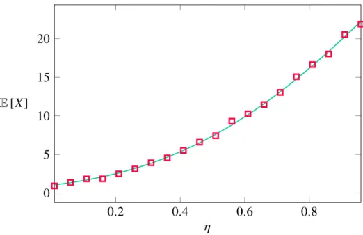
F(σ) =η·d(σk,σ₀)+xσ_k (1.4) Where η represents the drift, d(·,·) is the Hamming distance and xσ_k are independent random variables generated by a fixed distribution. Clearly, by the introduction of an arrow of evolution that favors successive mutations, the expectation value of accessible paths should be much higher than in the HoC model.

Indeed, in the case of Gumbel distributed random variables, it can be shown that [5]:

E[X]= L! 1−e⁻^ηL

Q_L

k=1 1−e⁻^ηk = L!

[L]!e⁻^η (1.5)

Where [L]!e⁻^η denotes the q-factorial. In the case of no drift whatsoever the RMF model corresponds to the HoC model and (1.5) reduces to (1.1), as expected.

Another interesting result for the RMF model: The probability to find an accessible path as a function of the genotype dimensionality approaches unity for any drift larger than zero [4].

If a mutation would be beneficial or deleterious, independent of all the other loci, studying fitness landscapes would become obsolete. Instead, the above models reflect the fact that the fitness of a mutation occuring at one locus depends on the allelic state of the remaining ones (i.e. a single mutation might either reduce fitness or increase it, depending on the state it originates from). As a consequence of this phenomena, called epistatis [16], local peaks may manifest on a given landscape, where all immediate mutational neighbors in the genotypic sequence space have a lower fitness associated with them, but, at larger Hamming distance, sequences with a higher fitness do exist.

(6)

0.2 0.4 0.6 0.8 0

5 10 15 20

η E[X]

Figure 1-1: The figure shows how the expected number of accessible paths varies under the RMF model with drift η. Fitness values are Gumbel distributed and the solid green line represents the analytical solution (1.5), whereas the numerical solution is indicated by square symbols. The hypercube dimension was set toL =5.

If a population happens to fix on such a local fitness peak, one way to escape it is through a drift-dependent stochastic sequential fixation process, where the whole population coincidentally moves toward lower fitness grounds (in order to reinforce the synonymity with a landscape, these lower grounds may be referred to as valleys). The rate of escape from a local peak under stochastic sequential fixation has been shown to decrease with population size [17, 14], which intuitively makes sense: The more individuals there are in a population, the less likely it is that all of them will be subject to the same mutation at the same time.

In a different approach for a population to escape a local peak, the requirement

(7)

Gillespie [6], who noted that the expected time for a population to divert from a local peak in such a process would decrease with the populations size. In the literature this mechanism is usually termed as a (deterministic) simultaneous fixation process or, since skipping genotypes of lower fitness resembles the quantum mechanical phenomenon where a particle tunnels through a potential barrier it could classically not surmount, ’stochastic tunneling’ [8].

In a first effort to formalize the above reasoning, we may formulate the combined waiting time for either of the two escape event to occur:

T_esc= 1

1/Tseq+1/Tsim (1.6)

011 111

001 101

010 110

000 100

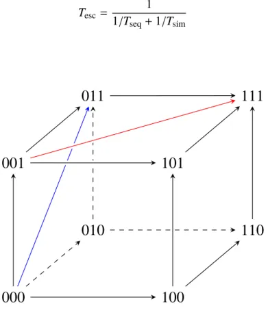
Figure 1-2: Shown is the Hamming space H₃² that contains all sequences of length three. Classically, a population can reach the global maximum (111) by mutating on each locus separately. By introducing escape processes, populations are provided with the possibility to leap over nodes in the hypercube (red and blue illustration).

(8)

000 100 010 001 110 011 101 111 Genotype sequence

Fitness−→

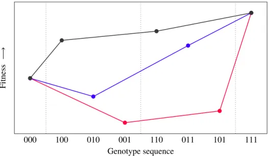
Figure 1-3: Shown are both of the two processes through which a population might escape a local fitness peak and, as a comparison, a classically accessible path. The dotted vertical lines delimit areas of equal Hamming distance. To enforce the absence of genetic mutation, once a genotype enters such an area, it may only leave it toward the right. In the drift-dependent stochastic sequential fixation process (the path that is colored in red) the whole population coincidentally moves toward lower fitness grounds, from where it will follow any path leading it to a higher fitness. Under a stochastic tunneling process, a fraction of the population mutates toward the valley genotype, only to be followed by mutation at other loci. If the secondary mutation turns out to lead to a higher fitness (compared to that of the escape genotype), a path is deemed viable in the stochastic tunneling model – this has been colored in blue. Classically, we demand all mutation steps to be beneficial, leading to a sequence of successively increasing genotype fitnesses (black path). Note that the three models may be seen as ordered by their restrictiveness, i.e.

the black one is allowed under all three models, blue is allowed only when stochastic tunneling is permitted, and red is allowed if and only if one allows a population to escape a genotype in a joint genetic drift event.

(9)

In the absence of back mutation (i.e. once a sequence mutates, it may not revert), it can be shown that both of the above processes are likely to occur in nature, and that in fact, depending on the size of a population, the combined waiting time (1.6) is dominated by either one. If a population happens to be smaller than a critical population size N_crit⁴, it will primarily escape local peaks through sequential fixation, whereas in populations larger than N_crit escape events will predominantly occur via stochastic tunneling [13].

Genotypic space Genotypic space

Fitness

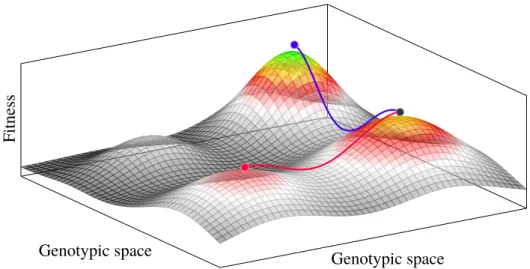
Figure 1-4: The above is a visualization of the relation between genotypes and their associated fitness, called a ’fitness landscape’. The genotypes are arranged along the x-y plane, the fitness is plotted on the z-axis. Note that S. Wright introduced this concept already noting that the above low- dimensional picture is a “very inadequate representation” [15] of the vast genotypic space. The landscape is somewhat rugged, several local peaks are separated by valleys through which a population may escape in two ways:

Under stochastic tunneling it may only mutate along the blue path, reaching a peak that has a higher fitness associated with it than the one it originated from. If the population happens to take a simultaneous downhill step, it may now move toward any of the peaks that are close by, even those that are lower in fitness than the one it escaped from (illustrated in red).

4The critical population size beyond which stochastic tunneling occurs predominantly can be approximated as a function of the mutation rate µand the fitness differential between local peak and escape genotype: N_crit≈log(s²_del(µs_ben)⁻¹+1)/(4s_del). Note that in the model that is used by Weinreich & Chao [13],s_delands_benare fixed.

(10)

Even though the two above processes are of different relevance depending on a given populations size, both will occur at a much lower rate than ordinary adaptive steps. In the simulations this lower likelihood is recognized by introducing an upper limit for the downhill steps available to a population.

If we, within the realms of the above mentioned models, proceed to allow direct paths along which a fixed number of mutations can be lept over, how are evolutionary accessibility and repeatability affected? As we relax the restraint that a path is only accessible in case the populations fitness along it increases monotonically, one could imagine said population to be crossing a fitness valley—thus the notion of ’downhill steps’ emerges. By speeding up the rate at which a population may mutate and thus departing the strong-selection-weak-mutation regime⁵, how is the constraint on the accessibility of the global maximum changed?

(11)

2 Algorithm

In order to retrieve the results that are evaluated in the next section, the algorithm that is normally used to scan the hypercube for accessible paths had to be extended in such a way that it included the ability to escape local peaks. The first step was to initiate fitness landscapes, i.e. each of the 2^Lgenotypes had to be assigned a fitness value. The number of paths – bound to increase by allowing downhill steps – was then found by a depth-first backtracking algorithm:

• Starting at the antipodal sequence (0000), lets say it moved forward toward a genotype with a higher fitness, e.g. (1000). Depending on the fitness associated with the next sequence, for instance (1100), it did either one of two things:

• In case (1100) also had a higher fitness associated with it⁶, the method moved forward to that sequence and recursively called upon itself to reini- tiate the search for paths toward the global fitness peak. This was the backbone of the algorithm, representing a single, fitness-increasing mutational step. Since such steps are allowed under all three models, this worked in the same manner, regardless of whether a population was allowed to perform downhill steps or not.

• When(1100)didn’t have a higher fitness associated with it, the algorithm reacted differently, depending on what type of escape mechanism was allowed, if any:

(a) In the drift-dependent stochastic sequential fixation process, the whole population moves towards a lower fitness value. If the population can reach higher fitness grounds from (1100), it will do so. As an implementation of this escape, the algorithm simply moved forward

6Computationally, this was realized by the use of a map that assigned each genotype a pseudo- randomly generated fitness. The pseudorandom numbers themselves were generated by using the Mersenne Twister [11].

(12)

to(1110), without comparing fitness values to the fitness associated with (1000). Having arrived at (1110) it then called upon itself, continuing its search for paths toward the global maximum. In order to prevent the algorithm from executing downhill steps repeatedly, a counter was raised. The algorithms behavior has been illustrated in Fig. 2-1, where the above situation corresponds with the red path.

(b) Only a small fraction of the population moves toward a lower fitness genotype in stochastic tunneling process, and it will be put under significant pressure by the remaining population. If the valley genotype cannot mutate toward a fitness value that exceeds that of the majority, it will simply die out under natural selection. To mirror the properties of a stochastic tunneling event, the fitness associated with (1000) was stored and compared to the fitness associated with genotypes that two additional mutations, for instance(1101). If by comparison the fitness associated with (1101) turned out to be greater than that of the local peak genotype(1000), the algorithm moved on to the escape sequence and, from there, continued its search for paths in the direction of the global maximum. In order to establish a limit on how many tunneling events were allowed, a counter was raised, likewise as has been done for (a).

(c) Classically, paths are only accessible if along it fitness values increase monotonically. On encountering a genotype with a lower fitness value, the algorithm did not have any means to overcome it.

(13)

(0000)

(1111)

(1000)

(1100) (1110)

(1101)

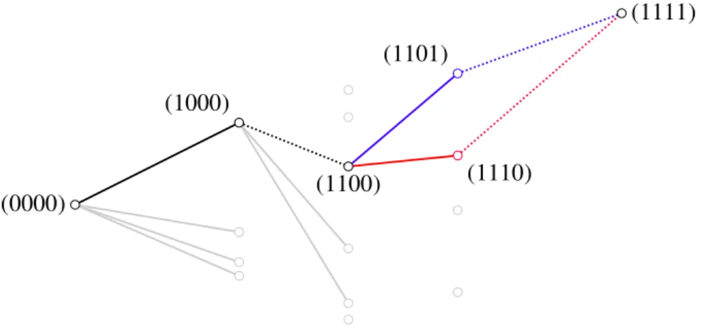
Figure 2-1: The above is an illustration of how the algorithm worked, that was used to count the number of accessible paths under either of the two escape models. Sequences correspond to nodes, who were grouped by their distance from the originating sequence and then aligned vertically in terms of their fitness. To improve visibility, only connections to nodes which may be reached from each genotype along the example path have been drawn⁷. Up to the sequence(1000)the algorithm moves along effortlessly, as the population undergoes a beneficial mutation in that step. Nodes (1110)and(1101)however cannot be reached without performing a downhill step, since the intermediate sequences fitness is smaller than that of the local peak genotype,(1000).

(1101) is in range in both a stochastic tunneling process (blue) and under stochastic sequential fixation (red). This is not the case for the (1110) sequence, since its fitness is lower than that of the local peaks sequence(1000).

Thus the algorithm will only move toward it under sequential fixation. In any case, a counter is raised on the event of the algorithm moving toward the valley genotype(1100). This prevents downhill steps from being applied continuously.

7After each mutation, a genotype can only mutate at all loci that so far remained unmutated.

Accordingly, the number of paths that lead out of a sequence grows smaller with increasing distance from the antipodal sequence.

(14)

Unfortunately, the maximum genotype dimension that the simulations could be realized for was generally smaller than in the classical model. This is for two reasons: On the one hand, comparing genotype fitnesses (under stochastic tunneling) was computationally expensive. Also, usually a lot more paths are found to be accessible when allowing a population to escape local peaks, which further increased the computational effort.

Since a discrete counter was raised to prevent the algorithm from executing multiple escape processes, a minimum number of escape processes was permitted, regardless of genotype dimension. As has been stated initially however, such processes are very unlikely to occur in comparison to a simple beneficial mutation.

This leads to two things: It made it unnecessary to increase the downhill step counter to values greater than one and, at least for very low genotype dimensions, the populations granted ability to perform a downhill step presumably imparts a positive bias on the overall evolutionary accessibility.

Unaffected by the above, in all simulations that calculate the probability not to find an accessible path the search algorithm was ended upon finding the first such path. This of course made this particular search a lot faster, allowing it to be run for larger genotype dimensions.

(15)

3 Results

3.1 Downhill steps on the HoC landscape

3.1.1 Probability not to find an accessible path

As has been underlined in the previous chapter, in all of the simulations just one downhill step was permitted; this appropriately reflects the fact that both escape processes will occur only with low probability. To analyse how evolutionary accessibility is transformed under the appliance of the two escape models, one may first take a look at the probability not to find at least one accessible path:

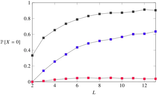
• Under the stochastic sequential fixation process, the probability not to find a path fluctuates around some small number. In other words, for both large and small hypercube dimension Lfinding a path remains likely.

• As a first indicator of how differently the observables behave within the models, the probability to find an accessible path with only stochastic tunneling allowed seems to diminish with the genotype dimension Lgrowing.

As simulations for genotype dimensions larger that thirteen were not computationally feasible, it is however impossible to assess whether this trend will hold. Besides that, its shape resembles that of the probability to not find an accessible path under the classical HoC model, where no downhill steps are allowed.

(16)

2 4 6 8 10 12 0

0.2 0.4 0.6 0.8 1

L P[X =0]

Figure 3-1: The figure shows how the probability to not find an accessible path behaves as a function of the genotype dimension. Both models that arise when downhill steps are allowed are represented: The blue line denotes the results for the stochastic tunneling model, the red line shows the (greater) likelihood to find a path when a population is allowed to escape via sequential fixation processes. As a benchmark, the black line was also included in the figure. It indicates the probability to not find an accessible path under the classical HoC model.

3.1.2 Expected number of accessible paths

The expected average number of accessible paths is bound to be larger than the known result for the classical HoC model (1.1). Also, as every path that is accessible under a stochastic tunneling process is also allowed in a drift-dependent stochastic sequential fixation process (see Fig. 1-3), we would expect the latter to facilitate the most paths.

(17)

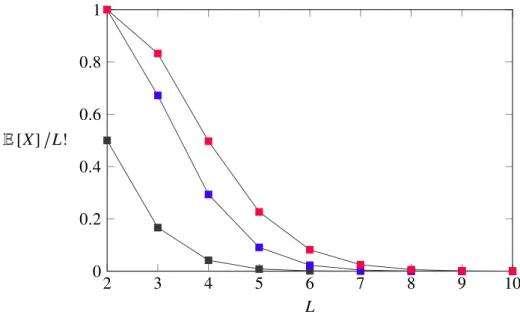
Due to the fact that the expectation value for the number of paths assumes an ever smaller fraction of the total paths available, instead of the actual number the ratio⁸ of accessible paths was plotted, see Fig. 3-2.

2 3 4 5 6 7 8 9 10

0 0.2 0.4 0.6 0.8 1

L E[X]L!

Figure 3-2: The figure shows the amount of paths that are accessible as a fraction of the total amount of paths in a hypercube of dimensionL. Although the expected number of accessible paths grows with larger dimensions, it miniaturizes in comparison to the total number of paths. As can also be seen from the figure, there will always be a greater number of paths when allowing stochastic sequential fixation processes (colored in red), since any path accessible under stochastic tunneling (blue) will also be accessible in a drift dependent escape process. For the HoC model (black) the ratio, which is simply 1/L!, approaches zero the quickest.

8The ratio is received by normalizing through the total number of paths in the hypercube of which there areL!.

(18)

In addition to displaying the fraction of accessible paths as a function of the genotype dimension, the de facto number of said paths may be expressed in terms of approximations:

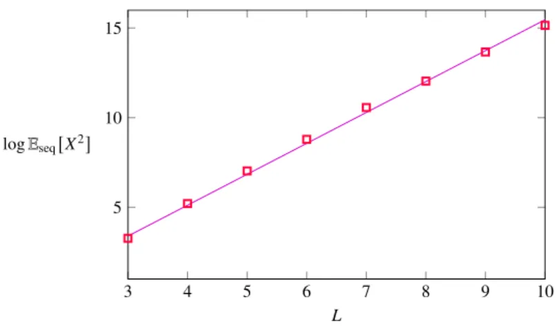
• As has been discussed with regards to Fig. 3-2, for all dimensions L the share of accessible paths is highest when a population is allowed to escape local peaks by stochastic sequential fixation processes. As is illustrated in Fig. 3-3, the actual number of paths grows exponentially. The parameters that guide the growth where approximated in a least square fit:

E_seq[X]≈ γˆ_seqe^α^ˆ^seq^L (3.1) 0.762< αˆ_seq < 0.788, 0.482 < γˆ_seq <0.519

• Although it does so slower for stochastic tunneling processes, the expected number of accessible paths does grow with the genotype dimension. By the same means as for (3.1), the average number of accessible paths may be approximated as a monomial in a fit:

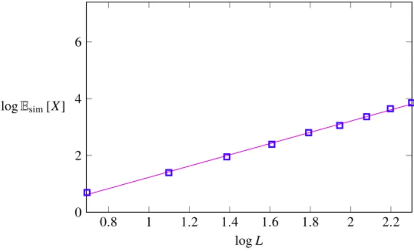
E_sim[X]≈ γˆ_simL^α^ˆ^sim (3.2) 1.955< αˆ_sim < 2.019, 0.419 < γˆ_sim < 0.522

(19)

2 3 4 5 6 7 8 9 10 0

2 4 6

L logE_seq[X]

Figure 3-3: The figure shows the logarithm to base e of the mean number of accessible paths. Under the stochastic sequential fixation process it grows exponentially. The least square fit that allows for the approximation under (3.1) is colored in magenta.

0.8 1 1.2 1.4 1.6 1.8 2 2.2

0 2 4 6

logL logE_sim[X]

Figure 3-4: As a function of the genotype dimensions, resized by its natural logarithm, the figure shows how the expected number of accessible paths – equally resized by applying the natural logarithm to it – behaves in the stochastic tunneling model. Growth is slower than under stochastic sequential fixation. However, as opposed to the classical HoC model where the expected number of paths equals one for arbitrary dimensions, the average number of paths does grow as a function of L. The magenta plot represents the least square fit of the approximation under (3.2).

(20)

3.1.3 Second moment of the number of paths

Similar to the expressions that were retrieved for the expectation value of the number of accessible paths, see (3.1) and (3.2), plots of the second moment as a function of genotype dimension can be approximated by least square fits:

• Under stochastic sequential fixation, the second moment will also grow exponentially as a function of L, as did the first. The fit returned the following parameters:

E_seqX²

≈ γˆ_seq⁰ e^α^ˆ⁰^seq^L (3.3) 1.694< αˆ⁰_seq < 1.753, 0.157 < γˆ_seq⁰ <0.183

• Similarly, for the stochastic tunneling model the growth rates of the first and second moment correspond. In fact, the second moment too will behave like a monomial expression when the a population is granted the ability to tunnel away from local peaks:

E_simX² ≈ γˆ_sim⁰ L^α^ˆ^sim⁰ (3.4) 5.960< αˆ⁰_sim < 6.107, 0.018 < γˆ_sim⁰ < 0.035

The expressions for the first and the second moment of the number of paths can sometimes be used to narrow down how the probability to find a path behaves in the limit of large hypercube dimensions. The following lemma, called the first- and second moment method, holds for random variables that only assume integer values [12, 7]:

E[X]≥ 1−P[X = 0]≥ E[X]²

EX² (3.5)

Unfortunately, the above yields the same non-result for both escape processes:

(21)

3 4 5 6 7 8 9 10 5

10 15

L logE_seqX²

Figure 3-5: Shown is the exponential growth of the second moment of the number of accessible paths in the stochastic sequential fixation model. The fit is colored in magenta, the data is denoted by red squares.

1.2 1.4 1.6 1.8 2 2.2

5 10 15

logL logE_simX²

Figure 3-6: If stochastic tunneling is allowed, the second moment as a function of genotype dimension L evolves as shown in this figure. Both axes were resized logarithmically. The data which was fitted with the parameters under (3.4) is indicated by the blue squares.

(22)

3.1.4 Combinatorial derivation for E

_seq

[X ]

In addition to showing that the expected number of paths in the sequential fixation model can be fitted by an exponential function, see (3.1), one can, by combinatorial arguments, derive an analytical argument for the exact number of paths. In order to calculate the number of paths by which the global maximum is accessible under sequential fixation, it is helpful to look at each path individually, of which there are a total of L! in the hypercube.

The main idea behind the derivation is the following: We condition on the probability that the k’th sequence has the lowest fitness associated with it— since the random variables are identically distributed and independent, this probability is 1/L. If the k’th genotype is located anywhere at a distance of 1 to L − 1 from the originating sequence, we know exactly where the downhill step has to be used, if the path is to be accessible (we only allow a single such step after all).

Therefore, all genotypes before the k’th entry have to be ordered, this is the case with probability 1/k!, as well as all the entries fromk+1 toL−1, which occurs with a probability of 1/(L−k −1)!. The final sequence is fixed, hence we do not have to consider it.

An exception to the above deliberations is the following: In case the very first genotype happens to be smallest, we have to consider the probability that the remaining L−2 genotypes are aligned in such a way that one downhill step will suffice to move along toward the global fitness maximum. As we do know that the first genotype is smallest, however, we also know that the first mutation will happen for certain. With the first step being guaranteed, reaching the global maximum

(23)

happens with the exact same probability with which the global maximum is reached in a hypercube of dimensionL−1. This yields the following recurrence relation:

P_acc(L)= 1 L

"

P_acc(L−1)+ XL−1 k=1

1

k! 1 (L−1−k)!

#

= 1

L

"

P_acc(L−1)+ 1 (L−1)!

L−1

X

k=1

(L−1)!

k!(L−1−k)!

#

= 1

L

"

P_acc(L−1)+ 1 (L−1)!

X^L⁻¹

k=0

L−1 k

!

− 1

(L−1)!

#

= 1

L

"

P_acc(L−1)+ 2^L−1−1 (L−1)!

#

(3.6)

Where we simplified by the use of the binomial theorem. Multiplying (3.6) with the overall number of paths in the hypercube then yields the expectation value for the number of accessible paths:

E_seq[X]

L = L!P_acc(L)= (L−1)!P_acc(L−1)+2^L−1−1= E_seq[X]

L−1+2^L⁻¹−1 (3.7)

For a genotype dimension of two, the global maximum is accessible via all available paths. We may solve (3.7) by applying that knowledge as our seed value:

E_seq[X]

L =

E_seq[X]

2+(4−1)+(8−1)+· · ·+(2^L−1) =

=

E_seq[X]

2+

L−1X

k=2

(2^k−1) =2+ 2^L −L−2

=2^L− L (3.8)

(24)

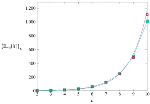
This result is compatible with the exponential growth by which the numerical solution was shown to behave in (3.1), which takes a similar form and also shows the ∝ 2^L behavior⁹; the prefactor in the approximation is incorrect however. In total, the result from the numerics was a good estimate of how the number of paths would behave with smallL, for large dimensions however the prediction turns out to be mistaken.

2 3 4 5 6 7 8 9 10

0 200 400 600 800 1,000 1,200

L E_seq[X]

L

Figure 3-7: The above figure shows that the analytical result (3.8), colored in green, and the numerical data retrieved by the algorithm (red squares) correspond. The fit to the data (magenta, see (3.1)) showed a similar growth, for largeL the quality of the approximation lessens, however.

9As a matter of fact, at approximately 2.173^Lthe approximation barely missed it. Nonetheless,

(25)

3.1.5 Analytical solution of E

_sim

[ X ]

By similar means we can argument for an analytical result when stochastic tunneling is allowed. Once more, we will split up the probability that an individual path is accessible by conditioning on a specific entry to be the smallest.

In the stochastic tunneling model crossing a valley is only allowed in the case of the escape genotype having a larger fitness associated with it. Therefore we have to enforce an additional limitation: Say we choose the k’th genotype along a path to be smallest. Then the genotype at k −1 has to be smaller than that at k+1. Since both the sequences before and after thek’th entry have to be ordered, the joint overall sequence (consisting of all but the k’th entry) has to be ordered as well. In accordance with this line of argument, we simply have to choose the single path that satisfies the above restrictions, of which there is just one in a total of(L−1)! permutations:

P_acc(L) = 1 L

fP_acc(L−1)+

L−1

X

k=1

1 (L−1)!

g =

= 1

LP_acc(L−1)+ L−1

L! (3.9)

Again, multiplication by the total number of paths L! yields a recurrence relation for the expected value of accessible paths in the stochastic tunneling model:

E_sim[X]

L =

E_sim[X]

L−1+L−1 (3.10)

(26)

2 3 4 5 6 7 8 9 10 0

10 20 30 40 50

L E_sim[X]

L

Figure 3-8: By looking at how the numerical data (blue squares) and the derived analytical result (3.11), denoted by green, compare, it can be seen that the latter is a very good assessment of accessibility in the stochastic tunneling model. The fit to the data (magenta, (3.2)) is shown as well, for dimensions up to ten it also very appropriately predicts the number of accessible paths.

For a genotype dimension of L = 2, it is impossible to assign fitness values in such a way that the global maximum will not be reached. Therefore, we may solve (3.10) with the same seed value as in the sequential fixation model:

E_sim[X]

L =

E_sim[X]

2+(3−1)+(4−1)+· · ·+(L−1) = 2+

L−1X

k=2

k = 1+ 1 2

L²−L

(3.11)

This result agrees with the fit to the numerical data, see (3.2), in which the prefactor and the exponent happen to turn out a bit smaller than the asymptotic behavior

(27)

3.1.6 Ratio of paths that make use of a downhill step

As has been mentioned in the introductory parts, in a classical fitness landscape, where no downhill steps are allowed, the expected number of accessible paths is constant at one for arbitrary genotype dimensions. In order to calculate the share of paths that were enabled only thanks to the availability of downhill steps r_dhs, one needs to simply subtract the expectation value to find a path in the HoC model from the expected value of accessible paths in either of the two escape processes.

Since they have been shown to grow without bounds in (3.8) and (3.11), it is easy to see that this expression approaches unity quickly for both models:

r_dhs ≡ E[X]−1

E[X] −→ 1 (3.12)

2 3 4 5 6 7 8 9 10

0 0.2 0.4 0.6 0.8 1

L rdhs

Figure 3-9: This plot demonstrates the fact that the ratio of paths that emerge thanks to the allowance of downhill steps quickly approaches unity for both models. It does so a bit quicker under stochastic sequential fixation (red), due to the fact that the expected value of accessible paths grows quicker under this process, see (3.8) and (3.11). The ratio for the stochastic tunneling model is colored in blue.

(28)

3.1.7 Distance at which downhill steps are performed

An additional question that arises is the following: Depending on the size of the genotypic space, at what Hamming distance from the antipodal sequence will the single downhill step usually be used up by the algorithm¹⁰? By making some simple combinatoric arguments, an estimate for the expectation value of that very distance can be calculated (for a derivation, see Appendix):

E[ddhs]= L−12^L⁻²−1

2^L⁻¹−1 (3.13)

3 4 5 6 7 8 9 10

0 2 4

L E[ddhs]

Figure 3-10: Shown is the expectation value for the Hamming distance at which the downhill step is used up as a function of the genotype dimension. In accordance with the analytical result (colored in green) for the upper boundary (3.13), the numerical result (red and blue squares) is always smaller, with the distance between the results (green squared boxes) increasing logarithmically. The latter has been approximated by a least square fit (magenta), which returned the parameters in (3.14).

(29)

There is however a caveat to the above results: The algorithm will regularly try to use a downhill step, even though it has done so earlier on. As this is prevented in the simulations, the number of downhill steps used at large distances from the original sequence decreases. This was not considered in the derivation, turning the above expression (3.13) into an upper limit forE[d_dhs]. The margin by which the expectation value is overestimated was fitted (see Fig. 3-10) and is of logarithmical growth inL:

∆E[ddhs]≈ log L^α^ˆ^dhs + βˆ_dhs (3.14) 0.238< αˆ_dhs < 0.260, −0.193 < βˆ_dhs < −0.139

0 1 2 3 4 5 6 7 8

0 0.05 0.1 0.15 0.2 0.25

d_dhs P[ddhs=k]

Figure 3-11: Shown are the analytical (green) and the numerical (red and blue squares) result, that the downhill step is used at a specific distance from the antipodal sequence. Compared to the analytical probability, the numerical result is shifted to the left, which is a consequence of introducing a counter that limits the number of available downhill steps. The hypercube dimension in the above simulations was set to ten.

(30)

3.1.8 Probability distributions

For a genotype space of fixed size, one can look at how probable it is that the algorithm will find a specific number of accessible paths. This has been done for dimensions five and seven:

• For the drift-dependent stochastic sequential fixation model, the probability distribution has a very long tail. This can be seen both from comparing it to the other distributions in Fig. 3-12 and 3-13 or, more clearly, from the fact that the cumulative distribution function approaches unity the slowest, see Fig. 3-14 and Fig. 3-15.

• When stochastic tunneling is allowed, large amounts of accessible paths are not encountered as frequently as under sequential fixation. Generally, the probability to find a greater number of paths than half of those available overall was very low. Within the 80000 fitness landscape realizations that were used to generate the distribution, only few to none (80 for a dimension of five, zero for seven) placed above that threshold.

• The probability distribution for the number of paths in the classical case has been included as well, in order to provide a context for the two above results.

As is expected, the distribution is centered around much smaller numbers and swiftly declines toward zero. Accordingly, its cumulative distribution function approaches unity the quickest.

The cumulative distribution functions have been calculated by successively adding up the probabilities of encountering a specific number of accessible paths. For a given genotype dimension L, they are defined as such:

F_L(Y)≡ X

P(X = X_i) (3.15)

(31)

0 20 40 60 80 100 120

−4

−3

−2

−1 0

X log₁₀P[X= k]

Figure 3-12: The probability distribution to encounter a given amount of accessible paths for a fixed genotype dimension of L = 5 under stochastic sequential fixation (red), stochastic tunneling (blue). Also, in order to make the two easier to compare, the classical model with no downhill steps (black) was included. As finding an accessible path is the easiest under stochastic sequential fixation (compare with Fig. 3-1), its distribution is broadest.

0 100 200 300 400 500 600

−4

−3

−2

−1 0

X log₁₀P[X= k]

Figure 3-13: Similar to 3-12 the probability distribution for the three different processes is plotted; this time at a larger genotype dimension of L = 7.

Although the curvature with which the distribution approaches zero for large X is different, the fact that under stochastic sequential fixation (red) this happens slowest coincides with what would be expected. Note that the total number of available paths 7! is a lot larger than the range in which the above plot is situated. Also shown are the distributions in the stochastic tunneling (blue) and the HoC model (black).

(32)

0 20 40 60 80 100 120 0

0.2 0.4 0.6 0.8 1

Y F5(Y)

Figure 3-14: The cumulative distribution function for a fixed genotype dimension of L = 5. It approaches unity quickest when no downhill steps are permitted (black) and has a comparatively long tail under stochastic sequential fixation (red). The blue curve indicates the result for the stochastic tunneling model.

0 1,000 2,000 3,000 4,000 5,000

0 0.2 0.4 0.6 0.8 1

Y F7(Y)

Figure 3-15: For a fixed genotype dimension of seven, all three cumulative distribution functions approach unity at a much smaller fraction of the total

(33)

3.1.9 Likelihood of an even number of paths

Under close inspection of Fig. 3-12 and Fig. 3-13, it stands out that the algorithm will more often than not find an even number of accessible paths for both of the escape mechanisms. This behavior however normalizes with growing genotype dimension, see Fig. 3-16 and 3-17. For a shorthand notation we define the following:

p_even ≡P["X even andX >0"] (3.16) p_odd ≡P["X odd andX > 0"] (3.17)

3 4 5 6 7 8 9 10

podd 1

/

²

peven

L

Figure 3-16: As a function of the genotype dimension, it can be seen how often the number of paths turned out to be even instead of being odd. For the drift-dependent stochastic sequential fixation, this ratio stabilizes around a value of one half for dimensions larger that seven.

(34)

3 4 5 6 7 8 9 10 p_odd

1

/

²

peven

L

Figure 3-17: Under stochastic tunneling, the probability that the algorithm returns an even number of accessible paths remains larger than the probability that said number is odd. Although the ratio steadily approaches one half, it does not reach it even for the largest realized dimension, which was ten.

3.2 Downhill steps in the α-HoC model

3.2.1 Probability to reach the global maximum

As has been mentioned in the introductory part, the analytical probability to find an accessible path in the α-HoC model is known, see (1.2). According to that result, for large genotype dimensions and smallα, there is always going to be an accessible path, whereas for largeα, there never is. In that sense, the probability to find a path toward the global maximum undergoes a phase transition at the critical value L⁻¹logL.

When we allow for either type of downhill steps to take place, this will naturally shift the phase transition toward larger values. This happens for one major reason: In the classical model the algorithm is faced with the task of immedi-

(35)

tunneling – the more restrictive¹¹ of the two escape processes – the algorithm already gets some leeway, as the distance to the global peak is reduced by one step (i.e. one less random variable is required to be larger thanα).

• As has been a trend in previous figures, the probability to find a path is largest for the stochastic sequential fixation process, given an arbitrary α.

Even in the extreme case of fixingαto one, the algorithm did – more often than not – reach the global peak. This largely different behavior (compared to the classical model) of the path-finding probability as a function of α is explained by the following argument: Even though the initial sequence is fixed at the maximum value, the population jointly drifts toward a lower valley genotype, ’forgetting’ that it had just been commonly occupying a genotype at a much higher fitness¹². The fact that the probability to find a path does start to decrease eventually is a result of choosingαso large that this will often force the available downhill step to be used up on the algorithms very first step; from here, all genotypes along an accessible path have to be nicely aligned, with their fitness increasing monotonically. In the extreme case ofα= 1, the probability to find a path in the sequential fixation model corresponds to that of the classical α-HoC with α = 0: In the classical model the initial fitness is fixed to the lowest value, this guarantees that the population will move toward any of one of the neighboring sequences, who all have a higher fitness associated with them. In the sequential fixation model, the initial sequence is a global peak and – relative to it – all neighbors have a lower fitness. As a result, the downhill step will be used on the first step. Therefore the initial mutation is ensured in both, and (as downhill steps are no longer available in the escape model) the number of accessible paths will be exactly the same.

11The α-HoC model corresponds to the method by which the random variables that shape a fitness landscape are drawn. Different from that, the two escape processes are simply means to navigate these landscapes. The argument that stochastic sequential fixation is the less restrictive escape process therefore remains completely intact.

12Oppositely, escaping an extremely large peak is near impossible under stochastic tunneling. In that sense, bacteria that form large populations have an advantage over small populations, as they will not accidentally drift away from a favorable evolutionary stance.

(36)

• Although finding an accessible path is more likely under stochastic tunneling for most α than for the classical model, once the initial fitness approaches one, the probability to find an accessible path will diminish completely.

When fixing the antipodal sequences fitness at such large values of α, the algorithm will be unable to find an additional, valley-separated genotype that tops the initial sequences fitness. Of course, for intermediate values, if escaping the initial sequence is necessary, the algorithm will most likely find a way to do so. Due to this a phase transition remains recognizable in the stochastic tunneling model, albeit for largerαthan in the classical model¹³.

0 0.2 0.4 0.6 0.8 1

α P[X >0]

Figure 3-18: The above probability to find a path as a function of the initial genotypes fitness is the result of simulations for genotype dimensions of seven (dotted), eight (dashed) and nine (dash dotted). Under stochastic sequential fixation, this probability starts to decrease only for very large α.

When simulating for large populations (therefore allowing only stochastic tunneling), the probability to find a path eventually approaches zero, albeit this happens for largerαthan in the classical model. Note that the probability to reach the global maximum in the classicalα-HoC model merges with that under sequential fixation, given the special case of αbeing fixed to zero in

(37)

4 Outlook

One question that immediately arises in the context of downhill steps is how evolutionary accessibility is affected if more than a single step is allowed. However, once we do allow additional downhill steps, a problem arises in terms of the escape processes classification, which had previously been of no concern: Do we allow more than one downhill step in a single escape¹⁴, essentially broadening the fitness valley that is traversed? Do we allow downhill steps that are initiated separately from each other, starting at two different genotypes? Or both?

Regardless of whether we are interested in escapes via sequential fixation or stochastic tunneling processes, the means by which we allow multiple downhill steps to occur have to be clarified in advance.

Distance from the antipodal sequence

Fitness

Figure 4-1: The two possible ways to spend more than one downhill step in order to reach the global maximum are illustrated for the stochastic tunneling model. The bottom path leads across a broader valley whereas, along the top path, smaller valleys are traversed. To improve visibility, in both paths the intermediate genotypes have been highlighted.

14By this, the weak mutation condition is weakened even further. A single genotype will now have enough time to mutate at two loci before being swept away by natural selection.

(38)

As it proves more complicated to clearly denote the processes that we want to allow, for some of the above combinations the computational realization will also turn out to be more of an extensive undertaking. This is especially the case for the stochastic tunneling model: Here, we save the fitness of the local peaks genotype in order to compare it to such sequences that are located across the valley. When increasing the number of allowed downhill steps, additional values have to be stored, which will add to the runtime of the search.

Implementing a larger maximum number of downhill steps (denoted bym_dhs) is of course easiest, when we do not consider whether these steps occur right after each other or not. From Fig. 4-2 it can be seen that the probability not to find an accessible path in the sequential fixation model vanishes already when allowing just two downhill steps¹⁵. It confirms ones intuition, that said probability becomes even smaller when further increasing the maximum number of downhill steps. The fact that it does so this quickly is however somewhat surprising.

2 4 6 8 10 12

0 0.05 0.1 0.15 0.2

L P[X =0]

Figure 4-2: For a maximum number of downhill steps m_dhs of one (red) and two (orange) the probability not to find a path is plotted against the size of the genotype space. Not finding a path proves very unlikely as soon as

(39)

Increasing the number of downhill steps in the stochastic tunneling model has a similar effect: The number of accessible paths increases by a significant margin.

As initially assumed, the runtime for the search turned out to be higher, the expected number of accessible paths was therefore only simulated for dimensions up to nine. The data from the numerics was fitted in a least square fit, which returned the following parameters:

E^II_sim[X]≈ γˆ_sim⁰⁰ L^α^ˆ^sim⁰⁰ (4.1) 4.472< αˆ⁰⁰_sim < 4.501, 0.030< γˆ_sim⁰⁰ < 0.031

From (4.1) it can be seen that, with an additional downhill step available, the exponent is more than twice as large as in the single downhill step expression, see (3.11). Naturally, if we had introduced one of the restrictions that were mentioned above (see Fig. 4-1) the fit would have returned a smaller exponent than that.

2 3 4 5 6 7 8 9

0 200 400 600

L E^II_sim[X]

Figure 4-3: In the stochastic tunneling model the number of paths (blue squares) grows significantly when the maximum number of downhill stepsm_dhs is increased to two. The fit that led to the parameters in (4.1) is colored in magenta.

(40)

Finding an analytical argument by similar means as for the single downhill step result proves a lot more complicated, as we are faced with an intricate web of nested recursions. However, the following argument can be made: As one would expect the multiple downhill steps to be performed in any out of a total of L^m^dhs combinations, each remainder of sequences would again have to be ordered, which happens with probability 1/(L − m_dhs)!. Multiplication by the total number of paths yields a term that is proportional toL^2m^dhs, which looks convincingly similar when compared to the above parameters.

As we do not explicitly consider paths along which neither (or any number smaller than the allowed maximum) of the downhill steps is used, this is only to be regarded as an estimate of how evolutionary accessibility behaves when increasing the number ofm_dhsto larger values.

(41)

5 Discussion

The models that were covered here represent the two ways by which a population can, in theory, escape a local peak on a fitness landscape. It has been shown that – in comparison to the classical HoC model – the probability to reach the global maximum significantly increased under the two escape models, see Fig. 3-1.

The prevailing mechanism in small populations is the drift-dependent stochastic sequential fixation process: The probability to find a path and the average number of such paths existing was determined to be largest when allowing this type of escape from local peaks. This was due to the fact that the algorithm did not have to check the feasibility of performing a tunneling action each time it encountered a lower fitness value; it simply moved along in all cases.

The fact that the expected number of paths was highest in the sequential fixation model can also be seen from comparing the escape mechanisms probability distributions (see Fig. 3-12 and Fig. 3-13) and their respective cumulative distribution functions (see Fig. 3-14 and Fig. 3-15). Under sequential fixation the algorithm had the best chances to find a large number of accessible paths, which resulted in its probability distribution having the longest tail and its cumulative distribution function converging to one slower than that for the stochastic tunneling model.

According to the fitted numerical data, see (3.1) and (3.3), the expected number of accessible paths and its second moment both exponentially grow as a function of the hypercube dimension for the stochastic sequential fixation process. Since the two did so at different speeds (the slope parameter in the fit for the second moment was roughly two and a half times larger), applying the first- and second moment lemma did not lead to any results.

For large populations, the probability that all its members drift toward a valley genotype becomes vanishingly small. Such populations may however still perform an escape from a local peak via stochastic tunneling. This too increased the probability to find a path and the mean number of such (again, relative to the classical HoC model).

(42)

The expectation value for the number of paths and its second moment in the stochastic tunneling model were fitted to the data from the simulations, see (3.2) and (3.4). It turned out that both of them grow in accordance with a power law;

only the second moment does so at an about three times quicker rate.

In addition to determining the growth of the number of accessible paths in both models, combinatorial solutions were derived, see (3.8) and (3.11). From these it can be seen that the number of paths asymptotically grows with 2^L if escapes via sequential fixation are allowed and it does so withL²/2 under stochastic tunneling.

Also, the analytical and the numerical results were shown to correspond very well, at least for smaller dimensions (see Fig. 3-7 and Fig. 3-8).

Since the expected number of accessible paths is fixed at one for all genotype dimensions in the classical HoC model, the ratio of accessible direct paths that arose only thanks to the possibility of performing a downhill step quickly approached unity, see (3.12).

Another observable that was of interest in the context of downhill steps was the distance from the originating sequence at which the algorithm would typically use them. An upper boundary was derived (3.13) and compared to the numerical data; in this manner the estimates error was shown to grow logarithmically as a function of the hypercube dimension.

An open question remains why, under both escape processes, more often than not the number of paths that were retrieved turned out to be even (see Fig. 3-16 and Fig. 3-17). Although this behavior seemed to normalize with growing genotype dimensions, it did take longer to even out in the stochastic tunneling model.

The behavior of the probability to find an accessible path as a function ofα in the α-HoC model was plotted for both escape processes, see Fig. 3-18. In the stochastic tunneling model, a similar phase transition as in the classical model was shown to occur, albeit at largerα. When allowing stochastic sequential fixation, the probability that the global maximum was reached was generally very high. Notably,

(43)

phase transition takes place could however no longer be identified, which was due to the fact that the algorithm would escape even the largest initial fitnesses. Once given a head start, at least one suitable path along which the global peak could be reached was then usually found.

When allowing multiple downhill steps to occur – without formulating any restrictions as to whether these may happen subsequently or in separate escapes – the probability not to find a path was shown to equal zero in the sequential fixation model, for all dimensions that were realized. For the stochastic tunneling model an argument was presented which suggested that the growth of the number of accessible paths behaves likeL^2m^dhs. This compared well to the fitted data, see (4.1).

In regards to the simulations, difficulties arose concerning the scaling of the genotype space: As the algorithm required a higher effort in terms of memory allocation, it was computationally unfeasible to generate data for dimensions larger than ten¹⁶. Also, the results were affected by the introduction of a distinct counter, which was necessary to reflect the fact that downhill steps are only performed with a limited likelihood. In an alternative implementation the algorithm could, each time it encounters a lower fitness value, draw a random number and compare this to some decision probability. Intuitively, that decision probability should be formed by comparing the likelihoods to perform an escape event and that to undergo a single beneficial mutation. Depending on that ratio, this method might however additionally increase the computational efforts required to scan the hypercube.

16In simulations where the exact number of accessible paths was of no concern, it was possible to raise the genotype dimension up to a value ofL=13.

(44)

6 Appendix

When deriving the expected value for the average distance at which the downhill step is used, d_dhs, we will be faced with two sums. The binomial theorem will be of help in rewriting them:

(x+y)^N = XN k=0

N k

!

x^N−ky^k (A1)

Another fundamental combinatorial technique that will be put to use is double counting:

N k

! k m

!

= N m

! N −m k −m

! _(m=1)

=⇒ k N k

!

= N N −1 k −1

! (A2)

Each genotype that differs atkloci from the originating sequence – of which there are _L

k

– may still mutate at L − k loci. Combining both of these expressions yields the number of connections N_k,k+1 along which a genotype at distance k from the originating sequence may mutate toward a genotype at distance k +1.

By multiplying with the corresponding distance from the antipodal sequence at which the downhill step is then usedd_dhs(k)(which is simplyk), one receives the expectation value at which the downhill step will be used on average (this still has to be normalized by the overall number of connections,N_tot). These considerations yield the first sum we are interested in:

N_tot·E[d_dhs]= XL−2 k=0

N_k,k+₁·d_dhs(k) = XL−2 d=0

k(L−k) L k

!

=

L−2

X k(L−k) L! X^L⁻² L−1!

(45)

Note that the above sum ends at a Hamming distance of L−2 from the original sequence, since a population will not perform a downhill step once it arrives at distanceL−1 (due to the fixing of the antipodal sequence). We now first apply (A2) to the above sum(I)and then rewrite by (A1), where xand yare equal to one:

L−1

X

k=0

k L−1 k

! (A2)

= (L−1)X^L⁻¹

k=0

L−2 k−1

!

= (L−1)X^L⁻¹

k=1

L−2 k−1

!

= (L−1)X^L−2

k=0

L−2 k

! (A1)

= (L−1)2^L⁻² (A4) By the combination of expressions (A3) and (A4) we receive the closed-form expression of the unnormalized expectation value for d_dhs¹⁷:

N_tot·E[d_dhs]= L²−L 2^L−2−1

(A5) Said normalization factor – which is equal to the total number of connections along which the downhill step could, in theory, be used – also has a closed-form expression:

N_tot=

L−2

X

k=0

N_k,k+1=

L−2

X

k=0

(L− k) L k

!

= L

L−2

X

k=0

L−k L

L!

k!(L−k)! = L

L−2

X

k=0

L−1 k

!

= L

L−1

X

k=0

L−1 k

!

−L ^(A1)= L

2^L⁻¹−1

(A6)

Insert this into (A5) and we arrive at the expression for the upper limit of the average Hamming distance at which the downhill step is used:

E[d_dhs]= L−12^L⁻²−1

2^L⁻¹−1 (3.13)

17Although it has not been explicitly mentioned yet, we wantLto only assume values larger or equal than two. Otherwise the above sums would not be well defined.

(46)

7 References

[1] Takuyo Aita, Hidefumi Uchiyama, Tetsuya Inaoka, Motowo Nakajima, Toshio Kokubo, and Yuzuru Husimi. Analysis of a local fitness landscape with a model of the rough mt. fuji-type landscape: Application to prolyl endopeptidase and thermolysin. Biopolymers, 54(1):64–79, 2000.

[2] Charles Darwin. On the origins of species by means of natural selection.

London: Murray, 1859.

[3] J Arjan GM de Visser and Joachim Krug. Empirical fitness landscapes and the predictability of evolution. Nature Reviews Genetics, 15(7):480–490, 2014.

[4] Jasper Franke, Alexander Klözer, J Arjan GM de Visser, and Joachim Krug.

Evolutionary accessibility of mutational pathways. PLoS computational bi- ology, 7(8):e1002134, 2011.

[5] Jasper Franke, Gregor Wergen, and Joachim Krug. Records and sequences of records from random variables with a linear trend. Journal of Statistical Mechanics: Theory and Experiment, 2010(10):P10013, 2010.

[6] John H Gillespie. Molecular evolution over the mutational landscape. Evo- lution, pages 1116–1129, 1984.

[7] Peter Hegarty and Anders Martinsson. On the existence of accessible paths in various models of fitness landscapes. The Annals of Applied Probability, 24(4):1375–1395, 2014.