Decay in Outgoing Null Directions of Solutions of the Massive Dirac Equation
in certain Asymptotically Flat, Static Spacetimes
Dissertation
zur Erlangung des Doktorgrades der Naturwissenschaften (Dr. rer. nat.)
der Fakult¨at f¨ur Mathematik der Universit¨at Regensburg
vorgelegt von
Jan-Hendrik Treude
aus Reutlingen
Dezember 2014
Die Arbeit wurde angeleitet von Prof. Dr. Felix Finster.
Pr¨ufungsausschuss: Vorsitzender: Prof. Dr. Bernd Ammann 1. Gutachter: Prof. Dr. Felix Finster
2. Gutachter: Prof. Dr. Jean-Philippe Nicolas (Universit´e Brest, France) weiterer Pr¨ufer: Prof. Dr. Stefan Friedl
Gegenstand der vorliegenden Arbeit ist die massive Dirac Gleichung auf gewissen statis- chen, asymptotisch flachen Lorentz-Mannigfaltigkeiten. Mittels analytischer Methoden f¨ur hy- perbolische Gleichungen wird untersucht, wie sich L¨osungen dieser Gleichung im Unendlichen der Mannigfaltigkeit, genauer im lichtartigen Unendlichen, verhalten. Spezieller geht es um die Fragestellung, inwiefern die Amplitude einer L¨osung im lichtartigen Unendlichen gegen Null kon- vergiert.
Die genaue Analyse verl¨auft unter der Einschr¨ankung auf glatte L¨osungen der Dirac Glei- chung, deren Tr¨ager r¨aumlich kompakt ist, sowie der Annahme, dass die zugrunde liegende Raumzeit statisch und asymptotisch flach ist. Außerdem ist es essentiell, dass die Masse in der Dirac-Gleichung ungleich Null ist. F¨ur solche L¨osungen wird dann bewiesen, dass ihre Am- plitude schneller als jede Potenz der auslaufenden lichtartigen Koordinate gegen Null konvergiert wenn diese Koordinate gegen unendlich strebt.
Eine spezielle Herangehensweise in dieser Arbeit ist, die Dirac Gleichung direkt in angepassten lichtartigen Koordinaten zu untersuchen. Dies f¨uhrt unmittelbar zu Methoden, die mit dem cha- rakteristischen Anfangswertproblem oder auch Goursat-Problem der Dirac Gleichung verwandt sind, sowie zu Energieabsch¨atzungen in Gebieten mit lichtartigen R¨andern.
Insgesamt gesehen ist die Herangehensweise eine st¨orungstheoretische, nahegelegt durch die asymptotische Flachheit der zugrunde liegenden Raumzeit: Zun¨achst wird die entsprechende Fragestellung im flachen Minkowskiraum bearbeitet, wo sich die Dirac Gleichung mittels Green- scher Funktionen l¨osen l¨asst. Anschließend wird darauf aufbauend die eigentliche Problemstellung mittels St¨orungstheorie behandelt. Dabei spielen Energieabsch¨atzungen, speziell die Ausnutzung der sogenannten Stromerhaltung der Dirac Gleichung, eine wesentliche Rolle.
Abstract
The topic of the thesis at hand is the massive Dirac equation on certain asymptotically flat, static spacetimes. Using analytical methods for hyperbolic equations, the behaviour of solutions of this equation at infinity of the manifold is analyzed, more precisely at so-called lightlike infinity.
Specifically, it is studied to what extent solutions decay to zero at lightlike infinity.
The concrete analysis is restricted to smooth and spatially compactly supported solutions, and is always under the general assumption that the underlying spacetime is static and asymptotically flat. Moreover, it is absolutely essential that the mass in the Dirac equation is nonzero. It is then proved that such solutions decay to zero faster than any inverse power of the outgoing null coordinate as that coordinate tends to infinity.
A particular approach taken in this thesis is to analyze the Dirac equation directly in adapted lightlike coordinates. This immediately leads to methods related to the characteristic initial value problem or Goursat problem for the Dirac equation, and to the use of energy estimates in domains with lightlike boundaries.
The general approach is to proceed by perturbation theoretic arguments, as is suggested by the asymptotic flatness of the underlying spacetime: First the question of decay is addressed in flat Minkowski spacetime, for which the Dirac equation can be solved rather explicitly by Green’s function methods. Building on this, the actual equation is then treated by a perturbation argument. In this argument, energy estimates play a crucial role, especially in form of the so-called conserved current of the Dirac equation.
In the following I would like to express my gratitude to people who played an impor- tant role during the time I worked on this thesis.
Most of all I want to thank my doctoral advisor Professor Felix Finster for his con- stant encouragement and for taking much time helping me throughout the various phases of my doctoral studies. I greatly benefited from his experience in many ways, not only concerning technical aspects, and our conversations about (mathematical) research in general, life as a researcher, and the high and low side of doing research were very valu- able to me. I also want to thank him for being the gentle and kind person he is, this made me feel very welcome in Regensburg and in his research group from the first day on.
Next, I want to thank Professor Jean-Philippe Nicolas for his interest in my work and the many useful inputs he gave me during his stay in Regensburg and the other occasions we met. I especially want to thank him for inviting me to Brest and taking the time to work with me and to show me the beautiful surroundings. Being able to discuss and exchange ideas with him was a big motivation and inspiration for me.
Then there are of course many different people in Regensburg who helped me during the last years and whom I want to thank.
I want to thank my secondary advisor Professor Bernd Ammann for his comments about my work, and generally for being there as another experienced person to talk to.
Special thanks go to my very pleasant office mate Olaf M¨uller for helping me with various questions about Lorentzian geometry, spin geometry etc., for proof-reading parts of this thesis, and of course for our many interesting discussions.
I am grateful to Johannes Kleiner for being an enrichment in many different ways, and for his constant reminder of the human side of doing science. I also want to thank him for proof-reading various parts of this thesis.
To my spin geometry learning companion Nikolai Nowaczyk I want to say thank you for exploring parts of these intriguing mathematical objects together with me.
I also want to thank Nicolas Ginoux for always being willing to answer my various
“beginners questions” about spin geometry over the years.
Moreover, I want to thank all other present and past members of the Mathematical Physics working group whom I got to know over the years – Andreas Grotz, Simone Murro, Moritz Reintjes, Christian R¨oken, and Daniela Schiefeneder – for their input and for giving our group seminars and other activities such a sympathetic atmosphere.
Maybe even more importantly, let me thank all the people who have prevented me from going crazy at times while doing mathematics (or trying to). Above all Rebekka.
Last but not least, I gratefully acknowledge the financial and academic support by the DFG-Graduiertenkolleg GRK 1692 “Curvature, Cycles, Cohomology” during the last three years.
and all people pursuing honest research interests.
Introduction iii
Notation and Conventions xix
Chapter 1. Geometric and Algebraic Concepts behind the Dirac Equation 1
1.1. Clifford Algebras, Spin Groups, and Spin Spaces 1
1.2. Spin Structures, Spinor Bundles, and the Dirac Operator 14 Chapter 2. Some Analytical Tools for the Dirac Equation on Lorentzian Manifolds 27
2.1. The Conserved Current 27
2.2. The Dirac Equation as Symmetric Hyperbolic System 30
2.3. A Collection of Further Methods 43
Chapter 3. A Class of Static, Asymptotically Flat Spacetimes 65
3.1. Definition and Causal Properties 65
3.2. Asymptotic Flatness Conditions at r=∞ 69
3.3. The Factorization of the Dirac Equation on these Spacetimes 70 3.4. Further Computations with the Dirac Equation on these Spacetimes 81
Chapter 4. Decay in Outgoing Null Directions 87
4.1. Outline and Summary of this Chapter 87
4.2. From the Dirac Equation to the Dirac Null System 88
4.3. Decomposition into Free Part and Perturbation 92
4.4. Treatment of the Free Part 95
4.5. Treatment of the Perturbation 112
4.6. Decay in Null Directions of Individual Angular Momentum Modes 123
4.7. Decay in Null Directions of General Solutions 136
Chapter 5. Outlook and some Open Questions 143
Appendix A. Miscellaneous Results in Lorentzian Geometry 147
Bibliography 155
i
The main topic of this thesis is asymptotic behaviour of solutions of the massive Dirac equation on a Lorentzian manifold. More specifically, for a certain class of asymptoti- cally flat spacetimes with a well-defined notion of outgoing null geodesics, the following question is studied:
How do solutions of the massive Dirac equation behave (decay) along these outgoing null geodesics as one moves out to infinity?
This introduction contains an overview of the thesis, as well as some information about the motivation behind studying the above question and relations to other topics. We begin by describing the main results of the thesis.
1. What are the Main Results of this Thesis?
The core part of the thesis consists in studying decay properties of solutions of the massive Dirac equation on spacetimes (M, g) which have the form
(M =Rt×(r0,∞)r×N g= (1 +A(r))2
−dt2+ dr2
+R(r)2gN . (∗)
Here (N, gN) is a compact Riemannian spin manifold and A, R∈C∞(r0,∞), for which we assume that R,1 +A > 0. One may notice that any such spacetime is a warped product over the 1+1 dimensional base Q=Rt×(r0,∞)r,gQ= (1 +A(r))2[−dt2+ dr2], with Riemannian fibre (N, gN), and warping function R. The “dynamically relevant”
information is contained in (Q, gQ) andR.
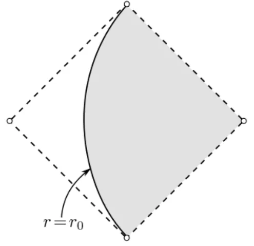
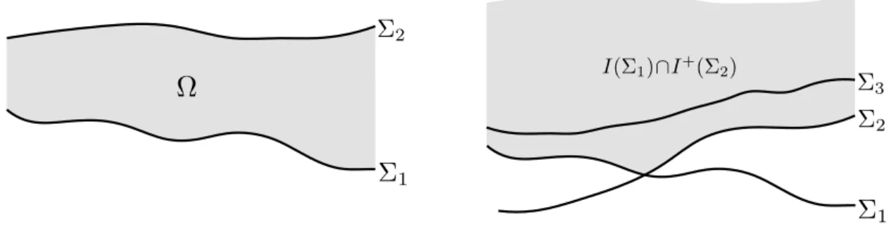
One can visualize such a spacetime as in figure 1 by a Penrose diagram for theQ-part.
Notice to this end that (Q, gQ) is conformally equivalent to a vertical stripRt×(r0,∞)r of Minkowski spacetime, and therefore has the same Penrose diagram.1 As the picture correctly suggests, (M, g) is globally hyperbolic if and only ifr0 =−∞. For the purpose of summarizing the results we focus on this case since it simplifies the statements while keeping the main point.
Besides being of this special form, we further assume that for some rm > r0 our spacetimes (M, g) satisfy the following two asymptotic boundedness and decay conditions:
i.) For anyk∈Nwe have
kA(r)kCk(rm,∞),kR−1kCk(rm,∞)<∞. ii.) There exists a constantC >0 and some α >0 such that
|A(r)|,|A0(r)|,|R−1(r)|,|(R−1)0(r)| ≤ C
(1 +r)α ∀r > rm.
1To be precise, we claim nothing about regularity of the conformally attached boundary. We only use the picture for the purpose of illustration, in particular of the null geodesics and the causal structure.
iii
Figure 1. Visualization of a spacetime as considered in this thesis.
A well-known example of a spacetime which satisfies all these conditions is the exterior Schwarzschild spacetime (cf. Example 3.2.2).
Concerning spinors, there is a correspondence between spin structures onM and on N such that the spinor bundle SM of M can be identified with the (pullback toM of the) direct sum SN ⊕SN of two copies of the spinor bundle of N. The Dirac operator then has the “block form”
DM = ie−a
11 0 0 −11
∂t+ ie−a
0 11
−11 0 ∂r+a0
2 + n−1 2
R0 R
+ i
R
0 DN DN 0
.
Here a∈C∞(r0,∞) is defined by the identity ea(r)= 1 +A(r). Using this formula it is possible to “split off” the explicit N-dependence by a separation of variables argument, which allows to restrict ourselves to the 1+1 dimensional partQ (with some “potential”
reflecting theN-part).
The main result stated below is concerned with decay of solutions of the massive Dirac equation. Since these are sections of a vector bundle one cannot directly speak of them being small or large. To do so, we use the following inner product: First, the spinor bundle SM is equipped with a non-degenerate, but indefinite Hermitian inner product
≺ ·,· SM in the fibers. Being indefinite this inner product is not well suited to capture the “size” of spinors. However, making use of the future-pointing unit-length timelike vector field T = e−a∂t onM, the inner product
h·,·iT :=≺ ·, γ(T)· SM
is positive definite. Here γ(T) denotes Clifford multiplication by T. We use this inner product to measure the size of spinors.
Finally, in the analysis of the resulting equation on Q (which takes up most of the work), we make crucial use of the null coordinates
v=t+r and u=t−r .
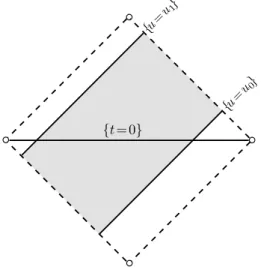
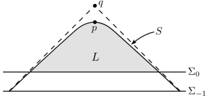
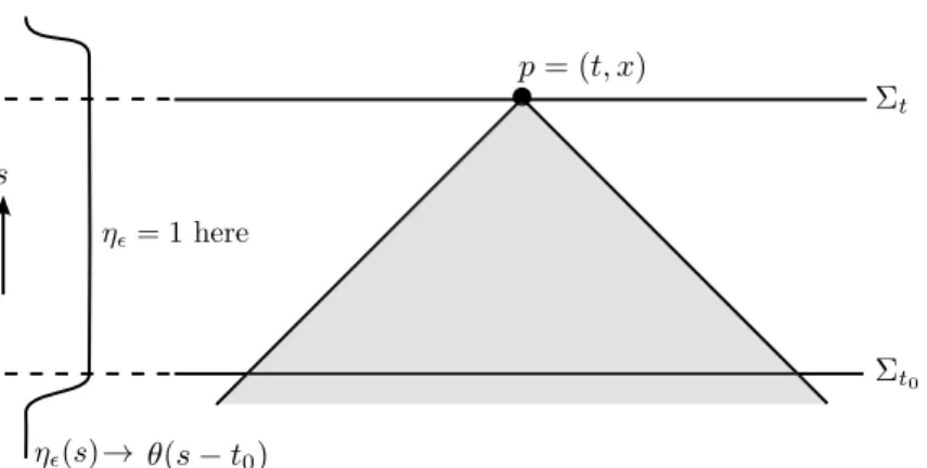
The main result is concerned with decay of solutions of the massive Dirac equation as the coordinatevtends to infinity, while the coordinateuis restricted to some finite range (concerning theN-dependence everything is uniform). Graphically speaking, we are thus making an estimate in a “null strip” as illustrated in figure 2. The precise result, in a version which is simple to understand, is as follows (cf. Corollary 4.7.5):
Figure 2. Illustration of a null strip in which the estimate takes place.
Theorem. (Superpolynomial decay in outgoing null directions) Let (M, g) be of the form (∗) with r0 = −∞, and assume that it satisfies the asymptotic conditions i.) and ii.). Fix a nonzero mass m 6= 0. Then for every k ∈ N and every u0 < u1
there exists a constant Ck>0 and a number s(k)∈N such that the following holds: Let ψ∈Γ∞sc(SM) satisfy (D−m)ψ= 0 andsuppψ|t=0⊂(−u1,−u0)×N. Then it holds that
|ψ(v, u, ω)|T ≤ Ck
(1 +v)kkψ|t=0kHs(k)(Σ) (∗∗) for all v > 0, u ∈ [u0, u1], ω ∈ N. Both Ck and s(k) depend on k, the constants in i.) and ii.), and Ck also depends on |u0−u1|and m.
Expressed in words, this result states that smooth, spatially compactly supported solutions of the massive Dirac equation decay as fast as any inverse power of v along outgoing null geodesics.
Let us say a few words about the methods which are used to obtain this result. The basic strategy is a perturbative one: First we explicitly solve a model equation derived from our actual equation of interest (the “free part”), whose solutions can easily be shown to decay as claimed in (∗∗). Afterwards, in the second, technically more demanding step we show that the difference between the model equation and the actual equation (the
“perturbation” or “error terms”) does not affect the behaviour (∗∗). More concretely, to carry out these steps the following general methods are used:
- For the free part, we useGreen’s function methods to derive an explicit integral representation formula for solutions of the model equation in terms of their (characteristic) initial data.
- To control the perturbation, we useenergy estimates in domains with lightlike boundaries, using the so-called “conserved current” of the Dirac equation. Here we also need to make use of the boundedness and decay assumptions of the metric stated earlier.
- To tie together the previous two parts, we use theLippmann-Schwinger equation (orDuhamel formula), see Section 4.6.1 and 4.6.2 for an explanation.
A more detailed outline is given below on page xvii of this introduction in the sum- mary of the fourth chapter.
2. What is the Motivation behind this Question?
The starting point for the work on this thesis was the article [MN04] by L. Mason and J.-P. Nicolas on conformal scattering in asymptotically simple spacetimes, which again builds upon ideas going back at least as far as to Penrose’s article [Pen65]. To explain this motivation, we start with a brief summary of [MN04].2
Conformal scattering in asymptotically simple spacetimes. In [MN04] the authors concentrate on globally hyperbolic spacetimes (M, g) with the following property:
One assumes that there exists an open, bounded, conformal embedding (M, g),→(M ,f eg) into a larger globally hyperbolic spacetime (M ,f eg) such that the following properties hold:
(AS1) Viewing M as subset of M, its topological boundary has the structuref
∂M ={ι+}∪˙ I+∪{ι˙ 0}∪˙I−∪{ι˙ −}, whereι+, ι−, ι0 ∈Mfsuch that
(a) ∂Ie−(ι+)∩∂Ie+(ι−) ={ι0}, whereIe± denote the causal future and past in (M ,f eg),
(b) I+:= ∂Ie−(ι+)\ {ι+, ι0} and I−:= ∂Ie+(ι−)\ {ι−, ι0} are two smooth null hypersurfaces of (M ,f eg).
(AS2) The conformal factor Ω, i.e. the smooth positive function on M withge= Ω2g, extends smoothly to all of Mf. Moreover, Ω|∂M = 0 and dΩ|I+∪I− vanishes nowhere, hence Ω is a boundary defining function for the smooth part of∂M. (AS3) Every future-directed, inextendible null geodesic in (M, g) acquires a future
endpoint on I+ and a past endpoint on I−.
The points ι+ and ι− are called future timelike infinity and past timelike infinity, the point ι0 is called spacelike infinity, and the null hypersurfaces I+ and I− are called future null infinity and past null infinity. Spacetimes (M, g) satisfying (A1)–(A3) are called (smoothly) asymptotically simple, and one should think of ∂M as a conformally attached boundary at infinity to such a spacetime.
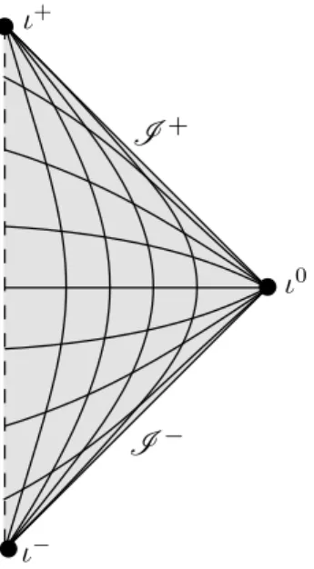
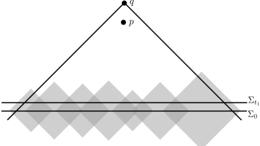
The basic example of a spacetime which satisfies these conditions is Minkowski space- timeR1,n, for which the so-calledPenrose conformal compactificationprovides the desired conformal embedding (see Appendix A.2). For this particular example the structure of the conformal embedding is illustrated in figure 3, where the angular coordinates are suppressed so that each point in the diagram should be thought of as representing an (n−1)–sphere. For a general asymptotically simple spacetime one should keep the same picture in mind. Besides Minkowski spacetime, other examples have been constructed by work of Friedrich, Corvino, Schoen, Chrusciel, and Delay (see [CD02] and references therein).
Now we come to the main point of [MN04]. Namely, if (M, g) satisfies the conditions (A1)–(A3), one can use this to study the asymptotic behaviour ofconformally invariant equations (or better, their solutions) towards the conformal boundary∂M in the follow- ing way: First of all, recall that a linear equation3 Pgφ= 0 on a vector bundle E over a
2For the sake of readability and in order not to distract from the main point to be made, the presentation in the following is a bit simplified concerning some technical aspects. In case of interest we refer the reader to the original article [MN04].
3Linearity is not crucial here, and conformal scattering constructions for nonlinear equations were carried out for instance in [BSZ90] and [Jou10, Jou12]. The analysis of course becomes more difficult then.
Figure 3. The schematic picture of an asymptotically simple space- time, thought of as being conformally embedded into 1 + 1 dimensional Minkowski spacetime. The horizontal lines represent Cauchy surfaces of
“constant time”, the vertical lines hypersurfaces of “constant radius”.
Since the embedding is conformal, (radial) null geodesics are still given by straight lines at 45 degree inclination angle.
Lorentzian, or more generally pseudo-Riemannian manifold (M, g) is said to be confor- mally invariant if for every conformal factor Ω∈C∞(M) there exists a transformation TΩ of the fields φ∈Γ∞(E) such that
Pg(φ) = 0 ⇐⇒ PΩ2g(TΩφ) = 0.
In other words, TΩ identifies the spaces of solutions of the two equations Pgφ = 0 and PΩ2gψ = 0. In most examples TΩφ = Ω−αφ for some α > 0. Some examples of con- formally invariant equations for which this is the case are the Maxwell equations, the massless Dirac equation, and the conformally coupled wave equation. These are pre- cisely the three equations considered in [MN04], so in the following we let Pgφ = 0 denote either of these equations.
Besides conformal invariance, another key property of these three equations is that they have a well-posed Cauchy problem if (M, g) is globally hyperbolic. Furthermore, they obey finite propagation speed according to the causality ofg. If (M, g) satisfies (A1)–
(A3), then one can combine these properties with conformal invariance of the equation Pgφ = 0 to smoothly extend any (rescaled) solutions of the equation Pgφ = 0 to the larger spacetime (M ,f eg) in the following way:
Let φ ∈ Γ∞sc(E) be a smooth, spatially compactly supported solution of Pgφ = 0.
Then TΩφ = Ω−αφ satisfies P
eg(TΩφ) = 0 since eg|M = Ω2g. Next, pick some Cauchy surface Σe ⊂ Mf which intersects M and extend (TΩφ)|
Σ∩Me smoothly to all of Σ (thise is possible since φ has spatially compact support). By global hyperbolicity of Mf, one can solve the Cauchy problem of the equation P
egφe= 0 in Mf, taking as initial data the extension of (TΩφ)|
Σ∩Me to Σ. Let us call the corresponding solutione TgΩφ ∈ Γ∞(E).e
Inside the original spacetime M it then holds thatP
egTΩφ= 0 andP
egTgΩφ= 0, and since TΩφand TgΩφcoincide on Σe∩M it follows from uniqueness of the Cauchy problem and finite propagation speed they two must actually coincide in M. Hence TgΩφ is indeed a smooth extension of TΩφ.
This seemingly simple observation has an interesting consequence concerning the asymptotic behaviour of spatially compactly supported solutions ofPgφ= 0 towards the conformal boundary ∂M. Namely, one just needs to combine the following two pieces of information:
i.) TΩφ= Ω−αφextends smoothly to ∂M,
ii.) Ω vanishes on∂M by (AS2), so Ω−α diverges towards ∂M (since α >0).
As an immediate consequence it follows that φmust decay to zero towards ∂M at least as fast as Ωα.
Actually even more can be said, at least for the massless Dirac equation and the Maxwell equation. For these equations, in a further step the authors of [MN04] identify the space of spatially compactly solutions of the equation Pgφ = 0 with their “traces”
on the boundary∂M. More precisely, after fixing a Cauchy surface Σ⊂M, consider the maps
T±: Γ∞c (E|Σ)−→Γ∞(E|eI±), φ0 7−→TgΩφ|I±,
where φ ∈Γ∞sc(E) denotes the solution of the Cauchy problem for Pgφ= 0 with initial data φ|Σ = φ0. Then, and this where most of the actual analysis is contained, it is shown that for certain naturally associated L2-Sobolev inner products on Γ∞c (E|Σ) and Γ∞c (E|eI±), the mapsT± are continuous linearisomorphisms between the spacesH and HI± obtained by taking the closure of Γ∞c (E|Σ) and Γ∞c (E|eI±) in the respective norm.
Notice that injectivity of the maps T± strengthens the previous decay result in the following way: Previously we only knew that any spatially compactly supported solution φ of Pgφ= 0 must decay to zero at least as fast as Ωα as one approaches ∂M. Now we can say that φ must actually decayprecisely as Ωα (unless φ= 0). Namely, otherwise (Ω−αφ)|∂M = 0, which by injectivity of I± can only hold if φ= 0.
Besides being interesting simply as far as understanding asymptotic properties of solutions is concerned, there are also other interesting applications. For instance, one may define the scattering operator
S :=T+◦T−:HI− −→HI+,
which maps an “incoming state” at past null infinityI−to the corresponding “outgoing state” at future null infinity I+ which results from the time evolution of the equation.
In this way one obtains a connection to scattering theory, which is the reason why the whole approach described up to this point is called “conformal scattering theory”.
It is basically a similar construction on which the principle of “holography” and the AdS/CFT-conjecturebuild, and conformal scattering theory can also be used to construct so-calledHadamard states in the framework of algebraic quantum field theory on curved spacetimes (for both, see the introduction of [DMP06] and further references therein).
The next part of this introduction contains more about the relation to usual scattering theory. For now, let us simply agree that the method of conformal scattering is of interest, and continue towards the actual topic of this thesis.
Conformal scattering for conformally non-invariant equations. One limita- tion of the conformal approach to scattering theory is of course its restriction to equations
which are conformally invariant. This for instance excludes the arguably most prototyp- ical wave equation on a Lorentzian manifold, the usual scalar wave equation gφ= 0 (i.e., theminimallyinstead of conformally coupled one). It also excludes allmassive equa- tions such as the Klein-Gordon equation (g−m2)φ= 0 or the massive Dirac equation (D−m)ψ= 0, which are crucial for Quantum Field Theory. Here m >0 is a parameter referred to as mass.
This limitation, or rather the question
Can the methods of conformal scattering theory be extended in some way to conformally non-invariant equations?,
was the original motivation for this thesis. Clearly for an arbitrary equation this seems unreasonable. But one might hope that if conformal invariance is broken only in some controllable way, then maybe the methods can still be suitably adapted. One natural class of equations for which this happens are “massive perturbations” of conformally invariant equations.4
For this reason, in this thesis we study the massive Dirac equation (D−m)ψ = 0.
Recall that the Dirac operator Dis conformally invariant in the following way: If M is spin with dimM =n+ 1, and ifeg= Ω2g are two conformally related Lorentzian metrics onM, then after suitably identifying the two spinor bundles the two corresponding Dirac operators DandDe are related by
De Ω−n2ψ
= Ω−n2−1Dψ .
Therefore, if ψ is a solution of the massive Dirac equationDψ=mψ, then the rescaled spinor field ψe:= Ω−n2ψ satisfies the equation
eDψe= 1
Ωmψ .e (∗)
So one sees explicitly that form6= 0 conformal invariance is broken by the fact that the mass term picks up a factor Ω−1.
Returning to the setup of asymptotically simple spacetimes, a crucial observation is that by (A2) the conformal factor Ωvanishes as one approaches the conformal boundary
∂M ⊂Mf. Consequently, the term Ω−1mblows up, illustrating that the equation (∗) for ψe has in some sense a “singularity” on ∂M. Since ∂M is precisely the place where we want to understand the behaviour of a solution ψ, the question is therefore:e
How does the singularity of Ω−1 on ∂M influence the behaviour of a solutionψe of (∗), defined on Mf\∂M, as one approaches ∂M?
In the following we are first going to present a rough analogue to (∗) which will suggest a particular type of behaviour of the solutions as one approaches the singularity.
Afterwards, however, we will argue why this analogy is perhaps not so good in the current situation and hence might be misleading. That it is indeed not a correct analogy is also confirmed by the results of this thesis.
First we describe the analogue to the Dirac equation. By assumption (A2) the con- formal factor Ω is a boundary defining function for the smooth partI±of the boundary.
Therefore it can be used as a transverse coordinate x0 = Ω to I±, i.e. it can be suitably completed to a set of coordinates (x0, x1, . . . , xn) such that the part of I± ly- ing in the corresponding coordinate domain corresponds precisely to the points p with
4The word “perturbation” is not quite sensible here since (as is seen in this thesis) introducing a mass term may substantially alter the properties of interest here.
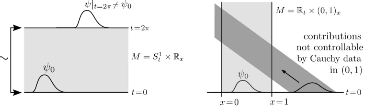
Figure 4. Level sets of the conformal factor Ω = 2 cosUcosV for the Penrose compactification of Minkowski spacetime into the Einstein cylinder. As the level sets illustrate, dΩ becomes lightlike towards I±.
x0(p) = Ω(p) = 0. Concerning the analogue to equation (∗), we write x = x0, simply ignore all the other coordinates (x1, . . . , xn) and also the vector-valuedness of the Dirac equation, and consider the ordinary differential equation
if0(x) = m
xf(x). (∗∗)
So in a sense we have replaced the Dirac operatorDe = ieγµ∇eµby idxd. Equation (∗∗) can of course be explicitly solved, and its solutions have the form
f(x) =c x−im =ce−imlogx.
Notice in particular that limx→0(f(x)·eimlogx) = c exists and may be viewed as a sort of “initial value off atx= 0” since one can recover f from the knowledge of this limit.
Going back to the rescaled Dirac equation (∗), this may be taken as a suggestion that perhaps a solutionψeof (∗) behaves likeψe∼Ω−im as one approachesI±. In other words, the suggestion is thatψewill simply oscillates faster and faster. If this were true, one could define “initial values” ofψealongI± by first dividing by this oscillating factor and then taking the limit of ΩimψetowardsI±.
Let us now give an argument for why it does not quite work like this in asymptotically simple spacetimes. Basically there is one simple reason:
The coordinatex0 = Ω is in a sense not a good “time direction” with respect to which the (massive) Dirac equation (∗) is hyperbolic.
Maybe the simplest way to make this statement more sensible is by pointing out that dΩ becomes lightlike along I± = Ω−1({0}), which are lightlike hypersurfaces (of Mf). For Minkowski spacetime this is illustrated by figure 4, where level sets of Ω are sketched.
For this reason, i.e. since they are not spacelike,I± are no natural hypersurfaces where one might pose initial values. To be more accurate, this is not quite true since some- times one can actually solve so-called characteristic initial value problems for hyperbolic equations, for which initial values are prescribed on a characteristic hypersurface instead
of a spacelike one. For instance this is actually done in [MN04], where solving such a characteristic initial value problem is a key part of the conformal scattering construction.
However, as far as the equation (∗) is concerned, the additional fact that mΩ−1 has a singularity on I± (for m6= 0) provides a rather convincing intuitive argument for why matters are different here:
For this argument, one views mΩ−1 as an infinitely high “potential wall” at I±, which prevents a solution of (∗) from reachingI±. Vividly speaking, at each spacetime point the solution can propagate along the causal directions into the future (timelike and lightlike ones). The lightlike directions are those which lead onto I+, whereas the timelike ones are those leading into ι+. Now the intuitive idea is that for m 6= 0 the infinitely high potential wall mΩ−1 prevents the solution from reaching I+, and rather
“pushes it intoι+”. Consequently, most of the wave should propagate intoι+ifm6= 0. In the massless case (m= 0) on the other hand, the solution may propagate “unhindered”
onto I+.5
Of course this is only an intuitive account of what might be going on around I+, and one should try to investigate to which extent this picture is actually correct.
The real starting point for this thesis. Making the previously outlined intuitive description more precise may be considered as the “real” starting point of this thesis and a way to understand its contribution. Namely, the question addressed in this thesis is precisely howψedoes in fact behave at I+.
The first attempt was to deduce asymptotic behaviour of solutions similar as for the analogue equation presented above. More precisely, the idea consisted in trying to rescale a solution in such a way that the rescaled solution satisfies (in suitable coordinates) some equation which can be continued to the boundary. As this more and more did not seem to work, the focus shifted towards studying decay properties by the usual methods for hyperbolic equations, i.e. by energy estimates. This then lead to the actual contents of the main body of this thesis, in particular to the result that a (spatially compactly supported) solutionψedecays “superpolynomially fast” towardsI+(see the summary of the results on page iii above for more details).
This indeed indicates that ψe does “not reach”I+ in the sense that it decays very rapidly. In a second step, it would of course be interesting to determine what precisely happens around the pointι+. This is still open for future research, some indications are made in Chapter 5.
3. What are some Relations to Other Topics?
In the following we describe some similar research topics and directions. Of course this is not meant to be an exhaustive overview over any particular field or fields. The aim is rather to provide some coarse orientation on the integration of the results into a larger context by elaborating on various related topics.
Scattering theory. As already mentioned, the results of [MN04] do not only yield precise decay properties of certain fields at null infinity, but also contain the construction of the “scattering operator” S : HI− → HI+ which maps between “asymptotic in- and out-states”. In the following, we use the example of scattering theory to give some further physical motivation.
5The fact that, at infinity, the massless Dirac equation is basically a transport equation along null geodesics guarantees that it indeed does so, see [MN04, p. 213].
Scattering theory can be used in many different specific situations, but the connecting underlying theme is always that one wants to understand the asymptotic behaviour of some dynamical system (for large times) in terms of a related, simpler dynamical system.
Such a system could describe the motion of particles, or the propagation of waves (as in this thesis), but also something rather different such as population dynamics. Scattering theory can be used to study such a system whenever there exists another, typically more simple dynamical system which approximates the first one in some asymptotic regime.
The point is that this second, simpler system should be explicitly computable (in some sense) and thus allow to say something about the actual system of interest, which typically will be too complicated to solve explicitly.
To stay within the range of this thesis, one may imagine some sort of waves propa- gating through a part of the universe (spacetime) which contains an isolated gravitating object such as a star, a collection of stars, a black hole, or similar. The waves could for instance be lightwaves described by Maxwell’s equations, or quantum mechanical waves (electrons) described by the Dirac equation. In any case, the dynamical system of interest is an equationP φ= 0 which describes the propagation of these waves in the given back- ground spacetime. Now the idea in the present setup is that far away from the isolated object, the background spacetime should resemble flat Minkowski spacetime more and more, so the same should hold for the propagation of waves. Mathematically this means that if P0φ= 0 describes the propagation of the same type of waves in flat Minkowski spacetime, then
P φ=P0φ+Rφ ,
whereRφbecomes negligible at large distances from the isolated object (it might contain terms proportional tor−1,r−2, . . . wherer is the distance to the object). Let us call the part where R is not negligible the “region of interaction”.
Moreover, certain solutions of the so-called “free equation” P0φ = 0 usually have a clear physical interpretation (“plane waves”), and it is often possible to analyze or decompose an arbitrary solution of P0φ = 0 in terms of these special ones. This then leads to the following pictures: One images a wave entering from far away into the region of spacetime where the isolated object influences strongly the propagation of waves.
While still far away, this wave can be interpreted in terms of these special solutions of the free equation. After a while the wave enters into the region, where the isolated gravitating object influences strongly its propagation. Here it may not be possible to give a clear interpretation of the wave. But after yet another while (some part of) the wave will move away from the isolated object, and after some more time be so far away from it that it can again be interpreted in terms of the special solutions of the free equation.
Now the idea behind the “scattering map” is that it simply assigns to each wave which enters the region of interaction the wave which leaves this region after some time. If one knows the action of this map on all possible incoming waves, then one understands effectively the way in which the isolated object influences wave propagation. Typically this means that the scattering mapS :{incoming states} → {outgoing states}should be a bijection.
So much for the physical picture behind scattering theory. In practice, what one really has to show of course depends very much on the particular problem and how it is formulated. The setup in which scattering theory is most developed is where the dynamics (for instance the propagation of waves) can be described in terms of a 1-parameter group of unitary operators on a Hilbert space. Such a dynamics is always generated by a self-adjoint operator H, called Hamiltonian, and, roughly speaking, the mathematics of
scattering theory in this framework consists in showing thatH is unitarily equivalent to another, more simple self-adjoint operatorH0. This operator is typically derived from H by neglecting certain terms which are believed to be “small” in some sense, and describes the free dynamics. There exists a large body of literature on this particular approach, some well-known textbooks include [DG97], [Yaf92, Yaf10], or [RS79]. Formulated in this way, scattering theory may be considered as a part of spectral theory for operators, so let us call it the “spectral approach to scattering theory”.
The spectral approach to scattering theory has also been used in the context of wave equations on Lorentzian manifolds by various people in the present and past, and it has lead to very interesting results (see for instance the introduction of [MN04] for a few references). While being very powerful, the spectral approach to scattering theory suffers from one drawback: It basically works only for equations which do not explicitly depend on time.6 In the setting of wave equations on Lorentzian manifolds this means that the underlying spacetime should admit a timelike Killing vector field. However, similarly as argued in the introduction of [MN04], from the standpoint of partial differential equations the asymptotic behaviour of waves for large times, i.e. for instance the structure of the solutions close to I+(whenever such a notion is available), should mostly depend on the asymptotic structure of the metric in that part of infinity and not so much on whether it depends on time or not (at least the parts of the waves which travel out to infinity). The reason for this is that differential operators are local. Therefore it might seem reasonable to believe that there should exist other methods besides spectral theory by which one can extract the asymptotic behaviour of these waves, and which continue to work also for spacetimes without a timelike Killing field.
To be clear, what onecannot give up is the assumption that the underlying spacetime should have some well-defined “asymptotic structure at infinity” which yields a sort of
“simpler comparison dynamics” in the sense of scattering theory as explained in the beginning. However, as the notion of asymptotically simple spacetimes from above shows, this is not necessarily tied to the existence of a timelike Killing field.7 Therefore, the proposal in [MN04] is that the conformal approach to scattering theory, as explained before, could provide an alternative to the spectral approach in these spacetimes, at least for certain equations. It was also shown in [MN04] that in case the underlying spacetime is taken to be Minkowski spacetime, the conformal and the spectral theoretic approach lead to the same scattering operator. This provides further affirmation that the conformal approach may indeed be a “correct way” to study scattering also on spacetimes without timelike Killing vectors. Since their paper [MN04], the authors have further pursued the conformal approach in [MN09], [MN12], [Nic13], and conformal scattering has also been studied for a nonlinear equation in [Jou10, Jou12] by a student of one of these authors. Of course, with the conformal approach one is restricted to conformally invariant equations, or one has to try to extend this approach in some way to other equations, which brings us back to one of the original motivations behind this thesis.
Analysis on manifolds with a structure at infinity. It is a common theme in the analysis of (partial) differential equations to study an equation in some “asymptotic regime” in which the equation simplifies. In this regime it is then often possible to make
6This is not completely correct, but it seems that the explicitly time-dependent situations which can be covered are rather limited.
7One could imagine that at least asymptotically there should exist a timelike “almost-Killing field”, which could re-open the door for spectral methods.
more specific statements about solutions of the equation. For instance, scattering theory as just explained fits into this scheme, the asymptotic regime being the region at large distance to the “interaction region” in this case.
One particular setup in which this general theme is used, and which relates very closely to this thesis, is the analysis on manifolds with a well-defined “asymptotic struc- ture at infinity”. Indeed, the particular spacetimes on which the Dirac equation is studied in this thesis have such a structure at infinity (see page iii of this introduction).
In the context of Riemannian geometry onnoncompact manifolds, a common theme is to study the spectrum (or other properties) of the usual differential operators like the Laplace or Dirac operator on manifolds which have some sort of asymptotic structure at infinity: Typical examples are asymptotically flat manifolds, hyperbolic manifolds, manifolds with cylindrical ends, manifolds with conical ends, and others. There exists a large amount of articles in this context, a number of references can be found in the introduction of the article [ALN04].
One basic idea of the analytic machinery used in these situations, which by now is rather well developed, is the introduction of an appropriate functional framework (Sobolev spaces, pseudodifferential operator calculi) which is adapted to the specific structure at infinity. A basic exposition of these ideas can be found in the textbook [Mel95] by Melrose under the keywords “scattering calculus” and “b-calculus”. This approach has been generalized by Ammann, Lauter, and Nistor in [ALN04, ALN07]
to so-called Riemannian manifolds with a “Lie structure at infinity”.
Studying spectral properties of various geometric differential operators on such man- ifolds is in fact closely related to the propagation of waves for certain wave equations on correspondingstatic spacetimes (cf. [Mel95]). This relation has been studied by various people, for instance by Melrose, Vasy, and Wunsch (cf. [Vas08, MVW08]).
If one wants to study wave equations on non-static (or non-stationary) spacetimes, it is a natural question whether perhaps one can make a good definition of a spacetime with an asymptotic structure at infinity which then allows to develop an adequate func- tional framework to study asymptotic properties of solutions of wave equations on such spacetimes as well. For the wave equation, some very interesting recent results in this direction were obtained by Vasy for asymptotically de Sitter like, asymptotically anti de Sitter like, and asymptotically hyperbolic and Kerr-de Sitter like spacetimes ([Vas10, Vas12, Vas13]), by Melrose, S´a Barreto, and Vasy for asymptotically de Sitter-Schwarschild like spacetimes ([MSBV13]), and by Baskin, Vasy, and Wunsch for asymptotically Minkowski spacetimes ([BVW12]). In these works the authors derive very precise asymptotic expansions and decay rates for solutions of the wave equation.
The approach is always in the spirit of introducing an appropriate (microlocal) func- tional framework adapted to the asymptotic geometry at infinity, and a basic paradigm is to study Fredholm properties of (non-elliptic) operators such as the wave operator on suitable functional spaces. Let us also mention the very recent work of Hintz and Vasy which uses similar ideas to study local and global existence for semilinear wave equations on asymptotically de Sitter, Kerr-de Sitter and Minkowski spacetimes ([HV13]), and for quasilinar wave equations on asymptotically de Sitter and Kerr-de Sitter spacetimes ([Hin13, HV14]).
Returning to the beginning of the second part of this introduction, also the definition of an asymptotically simple spacetime provides a definition for an asymptotic structure at infinity. As explained, it uses ideas from conformal geometry and allows to study asymptotics of solutions of conformally invariant wave equations. In a similar spirit,
i.e. using conformal geometry (but in a more elaborate way), Gover and Waldron have recently developed a “boundary calculus” for equations on conformally compact pseudo- Riemannian manifolds of arbitrary signature ([GW14]). Similar to the ideas explained in the second part of the introduction, here one tries to relate solutions of equations in the original manifold to certain “boundary values” on the boundary of the conformal com- pactification. As also mentioned before, this has relations to the AdS/CFT-conjecture, see the introduction of [GW14]. Trying to use the approach of Gover and Waldron to study asymptotic (decay) properties of solutions of wave equation in the Lorentzian case is recent ongoing work.
Decay of linear waves. For linear hyperbolic equations, for which existence and uniqueness of solutions is well-understood in many cases, decay or more generally asymp- totic behaviour of solutions is one of the remaining general questions about its solutions one can always attempt to study. For various different equations this has been and still is continuously studied by many people for different reasons. Besides being interested in decay properties for their own sake, one commonly encountered motivation is that one wants to use decay properties of solutions of linear equations for studying nonlinear perturbations of these equations (see for instance [Tao06, Ch. 3]).
Instead of only restricting to nonlinear perturbations of linear equations, one may of course also start from a genuinely nonlinear equation and try to approach it by studying various linearizations. Here the paradigmatic example which fits into the general rela- tivistic context of this thesis are the Einstein equations. For these, one of the current aims is to prove stability of certain special solutions, most notably the Kerr black hole spacetime, under perturbations of their initial values. Here “stability” means stability of their global geometric properties such as geometric (in-)completeness or asymptotic falloff properties of the metric (similar to those of asymptotic simplicity). The approach of first studying decay properties of solutions of linear equations (on these specific space- times) has been successful for Minkowski spacetime (cf. [CK93]). We refer to the review article [CGP10, Sec. 6] for more details. In this spirit, one may view any decay result for a wave equation on a curved spacetime which can be coupled to the Einstein equations as a sort of naive “linear stability result” for the coupled system of that wave equation and the Einstein equation.
Coming back to decay estimates for linear equations and to the massive Dirac equa- tion in particular, let us mention the work of Finster, Kamran, Smoller, and Yau on the massive Dirac equation on certain black hole spacetimes like the Kerr-Newman spacetime ([FKSY02, FKSY03, FKSY09] or the Reissner-Nordstr¨om spacetime ([FKSY00]).
Here the original question was whether there can exist “bound states” of the massive Dirac equation on these spacetimes, i.e. solutions which remain localized in some bounded domain. These would correspond to the quantum mechanical analogue of classical plan- etary orbits. To answer this question, the authors studied the decay of local energy as time tends to infinity. The existence of bound states would mean that local energy does not decay. The methods used by these authors are quite different compared to the ones described before in that they derive an explicit integral representation of the Dirac propagator, i.e. the time evolution operator defined by the Dirac equation. This leads to certain Fourier-integrals which the authors estimate by the “saddle-point method” in the limit where time tends to infinity. In this way the authors manage to show that local energy and actually also the solution itself (at any point in space) decay liket−56 as t→ ∞. The interpretation of this is that the wave propagates into the black hole and/or
escapes to infinity. Compared to the decay results in this thesis, one may note that the limitt→ ∞(at fixedx) corresponds to approaching timelike infinityι+. The slower de- cay in timelike directions compared to the superpolynomial decay in lightlike directions obtained in this thesis reinforces the picture that the solution propagates mainly into ι+ instead ofI+. It is interesting to ask whether one can somehow describe these two decay properties together in a more uniform way.
4. Brief Summaries of the Individual Chapters
To finish up this introduction, we present a brief summary of the content of the individual chapters of the thesis. Basically the first two chapters contain background information to make the whole thesis more self-contained and to put the content into a larger context. In practice they also contain material, especially about the Dirac equation, which seems to be commonly known but is hard (or maybe not at all) to find in the existing literature. Nevertheless, the main new contributions of this thesis are contained in the third and fourth chapter. In particular Chapter 4 contains the whole analytical treatment of the problem.
Summary of Chapter 1. The basic objects of interest in this thesis are spinors on Lorentzian manifolds, a concept which is geometrically somewhat involved. The first chapter serves as brief introduction into the definition of spinors in order to make the thesis more self-contained, and also to give readers without background knowledge about spinors at least a small impression of the general algebraic and geometric underpinnings of the concept of a spinor.8
In practice there exist different, equivalent approaches to spinors (see the Introduc- tion of Chapter 1). In this thesis we follow the representation-theoretic approach using Clifford algebras, spin groups, and the spin representation on the algebraic side, and spin structures as well as the machinery of principal bundles and associated vector bundles on the geometric side. This approach has the advantage that it works in any dimension (and signature). All necessary concepts will be touched upon in the first chapter, although sometimes of course only very briefly. The hope is to provide a readable, sometimes intuitive (often quite dense) summary, which is understandable for readers having no background knowledge about spinors, and is a nice repetition for readers who are already familiar with spinors.
Summary of Chapter 2. In the second background chapter some general methods regarding the analysis of hyperbolic equations on Lorentzian manifolds are presented.
The focus is on the Dirac equation, and the methods explained here in a general context are used later in the thesis in specific situations. In short, the methods presented are:
- Energy estimatesin a geometric fashion, involving theconserved current of the Dirac equation, the energy-momentum tensor formalism, and related ideas, - Symmetric hyperbolic systems, a general type of hyperbolic equations which
applies to the Dirac equation and can be used to treat the Cauchy problem and finite propagation speed,
- Representation formulas for solutions of (some) hyperbolic equations in terms of their initial data, which can be obtained by Green’s function methods.
8It should be pointed out that the actual analysis in Chapter 4 starts with a concrete equation, and one should be able to follow it without any (or at least not too much) knowledge about spinors.
Many of the methods summarized in this chapter are used later in Chapter 4. Al- though Chapter 4 is written sufficiently detailed to be readable on its own, the presenta- tion in the second chapter embeds the methods used there into a larger context. The hope is that in this way the approach taken in this thesis is given a more methodical touch. In particular, Chapter 2 could be informative for potential readers with little background knowledge about hyperbolic equations by helping them understand the methods used later in the thesis in a somewhat more general context.
Of course, most of what is written in Chapter 2 is standard material about hyperbolic equations and can be found in most textbooks of the subject, as cited in Chapter 2.
However, applied specifically to the Dirac equation it is difficult (or not possible) to trace back some of the parts of this chapter to the existing literature even if these parts seem to be common knowledge. For this reason the chapter contains a number of detailed, although elementary computations for the Dirac equation, for instance concerning energy- momentum tensors.
Summary of Chapter 3. With this chapter the actually new contributions of this thesis start. In a sense, the third chapter prepares the stage for the analytical investiga- tions of Chapter 4, which make up the largest part of the thesis. Namely, Chapter 3 is concerned with the structure of the particular spacetimes on which we analyze the Dirac equation, and the form of the Dirac equation on these spacetimes.
Concretely, in the first part of Chapter 3 we introduce the class of spacetimes we consider, and describe their causal properties as well as the asymptotic conditions at infinity which we impose. Alongside we also describe some examples from the literature which fit into this class of spacetimes.
In the second part of Chapter 3 we study spinors on these spacetimes, deriving for instance a convenient expression for the Dirac operator in “block form” (see page iv of this introduction). Moreover, we derive various explicit formulas for Clifford multiplication, the spin connection, and inner products on the spinor bundle.
In the last part of this chapter we first show how the Dirac equation can be further simplified by making a conformal rescaling of spinor fields. Afterwards we introduce certain pointwise, L2, and Sobolev inner products on spinors, which are going to be used in the analysis of the fourth chapter. At the end of the chapter we also study how the current of a solution of the Dirac equation behaves in presence of the “interior boundary”
atr =r0 of these spacetimes (see figure 1), i.e. when it is conserved or not.
Summary of Chapter 4. This is the core chapter of the whole thesis, which con- tains all the analytic work. Let us therefore give a brief overview over the different parts of this chapter.
Section 4.2 starts with the previously mentioned Dirac operator in “block form” (and after the conformal rescaling mentioned above), and rewrites this further. The main step consists in separating off the N-dependence in the equation (recall that M =Rt× (r0,∞)r×N). Concretely this is done by projecting the Dirac equation (D−m)ψ= 0 onto anL2(SN)-orthonormal basis of eigenspinors of the Dirac operatorDN ofN, which works very conveniently using the block form of the Dirac operator.9 Each projected equation has the structure of a Dirac equation in flat 1+1-dimensional Minkowski spacetime with an “external potential” reflecting the presence ofN and the massm >0. As such, each equation is a pair of two transport equations which are coupled by the “potential”. In
9That this can be done in the first place relies on the fact that the Dirac operator on a compact Riemannian manifold is elliptic and (essentially) self-adjoint onL2 with discrete spectrum.
order to study these equations analytically, we transform to null coordinates v and u as introduced on page iv of this introduction. Expressed in these coordinates the Dirac equation takes a particular form which we refer to as the Dirac null system.
In the next step, in Section 4.3 we decompose the Dirac null system into two parts:
One part contains the (as it turns out) relevant terms for our purposes but at the same time is sufficiently simple such that it can be solved explicitly. It is called the “free part”.
The second part, the “perturbation”, contains all other terms which in the end turn out to be “small” compared to the free part. Let us point out that the free part also contains the mass m6= 0, which is crucial for the decay properties.
Having made this splitting, in Section 4.4 we explicitly solve the free part. Here the key observation is that the free part is in a sense equivalent to theKlein-Gordon equation in flat 1+1 dimensional flat Minkowski spacetime. For this reason it is possible to derive a representation for its solution in terms of a convolution integral of their initial data with the Green’s function of the Klein-Gordon equation. Using this formula and the specific form of the Green’s function, it is possible to directly estimate the decay of solutions as v tends to infinity. Here it is crucial to have a nonzero mass, otherwise the decay properties would not be as strong as obtained here (which is superpolynomially fast).
The following Sections 4.5 and 4.6 consist of showing, by a perturbative argument based on theLippmann-Schwinger equation (see Sec. 4.6.1), that the perturbation terms do not alter the decay properties for v → ∞. This is achieved by various energy esti- mates, which in detail are rather complicated but in principle simply combine current conservation of the Dirac equation as useful a priori estimate with the decay properties of the metric coefficients at infinity. How these estimates can then be combined with the decay properties of the free part by the Lippmann-Schwinger equation is outlined in Section 4.6.2 and carried out explicitly in Section 4.6.4.
The previous steps yield decay of solutions of the projected parts of the full Dirac equation ofM. Finally, in Section 4.7 we combine these decay estimates into an analogous estimate for solutions of the full Dirac equation on M. As indicated before, here it is crucial that we projected onto anL2-orthonormal eigenbasis ofDN. Namely, this together with having explicit control of the separation constants (the eigenvalues of DN) in the estimates for the projected equations allows to “sum up” these individual estimates using Parseval’s theorem. This then finally establishes the main result obtained in this thesis.
In the following one finds a list of some general notations and notational conventions used throughout this thesis. Mostly we follow standard conventions of the respective fields.
General conventions
- The signature of a Lorentzian metric is (−+· · ·+).
- The Clifford relations are defined with sign conventionvw+vw =−2hv, wi.
- Both index-free and abstract index notation are used throughout this thesis.
For instance, the (covariant) divergence of a symmetric 2-tensor T = Tµν is denoted by divT =∇µTµν.
- The Einstein summation convention is used. Greek indicesα, β, µ, ν, . . .usually run from 0 ton, and Roman indicesi, j, k, `, . . . run from 1 ton.
- We sometimes write Xx for a set X whose points are denoted by x to stress the notation for the points. For instance, we commonly writeRt×Σx.
- In estimates, numerical constants may change from line to line without this being explicitly stated.
Notation related to general differential and pseudo-Riemannian geometry (Mp,q, g) Pseudo-Riemannian manifold of signature (p, q)
(M, g) Pseudo-Riemannian manifold of some signature
SO+(M) Bundle of oriented and time-oriented orthonormal frames of (M, g) dµg Volume measure of a pseudo-Riemannian manifold (M, g)
I±, J± Timelike and causal future and past (in Lorentzian signature) dµΣ Induced volume measure on nondegenerate submanifold Σ⊂(M, g) νΣ Unit-normal to nondegenerate hypersurface Σ⊂(M, g)
Γ∞(E) Smooth sections of a vector bundle E Γ∞c (E) Compactly supported smooth sections
Γ∞sc(E) Spatially compactly supported smooth sections
ΓL2(E) L2-sections (w.r.t. some inner product and volume measure) ΓD0(E) Distributional sections
Notation related to Clifford algebras and spin groups
Rp,q Rp+q equipped with canonical inner product of signature (p, q) SO+(p, q) Time- and space-orientation preserving orthogonal maps ofRp,q Cl(p, q) Real Clifford algebra in signature (p, q)
Cl(n) Complex Clifford algebra in dimensions n {·,·} Anticommutator of two endomorphisms Spin+(p, q) Proper spin group in signature (p, q) ϑp,q Spin covering ofSO+(p, q) bySpin+(p, q)
xix
Sp,q Space of spinors in signature (p, q) ρp,q Spin representation of Spin+(p, q) onSp,q
γSp,q Clifford multiplication of Rp,q onSp,q
≺ ·,· Sp,q Spin+(p, q)-invariant Hermitian inner product onSp,q. Notation related to spinors
Spin+(M) Spin structure for (M, g)
SM Classical spinor bundle of (M, g) (w.r.t. some spin structure)
≺ ·,· SM Natural Hermitian inner product on SM γ(X) Clifford multiplication by X∈T M on SM
∇S,∇SM,∇ Spin connection on SM
DM,D Classical Dirac operator on SM Notation related to analysis
k·kLp
x(Ω) Lp-norm on a space Ω whose points are denoted by x k·kHk
x(Ω) Sobolev-type norm of orderk on a set Ωx k·kCk
x(Ω) Ck-norm on a set Ωx