Spin-charge coupled dynamics driven by a time-dependent magnetization

Spin-charge coupled dynamics driven by a time-dependent magnetization

Sebastian T¨olle,¹Ulrich Eckern,¹and Cosimo Gorini²

1Institut f¨ur Physik, Universit¨at Augsburg, 86135 Augsburg, Germany

2Institut f¨ur Theoretische Physik, Universit¨at Regensburg, 93040 Regensburg, Germany (Received 14 November 2016; revised manuscript received 3 February 2017; published 2 March 2017) The spin-charge coupled dynamics in a thin, magnetized metallic system are investigated. The effective driving force acting on the charge carriers is generated by a dynamical magnetic texture, which can be induced, e.g., by a magnetic material in contact with a normal-metal system. We consider a general inversion-asymmetric substrate/normal-metal/magnet structure, which, by specifying the precise nature of each layer, can mimic various experimentally employed setups. Inversion symmetry breaking gives rise to an effective Rashba spin- orbit interaction. We derive general spin-charge kinetic equations which show that such spin-orbit interaction, together with anisotropic Elliott-Yafet spin relaxation, yields significant corrections to the magnetization-induced dynamics. In particular, we present a consistent treatment of the spin density and spin current contributions to the equations of motion,inter alia, identifying a term in the effective force which appears due to a spin current polarized parallel to the magnetization. This “inverse-spin-filter” contribution depends markedly on the parameter which describes the anisotropy in spin relaxation. To further highlight the physical meaning of the different contributions, the spin-pumping configuration of typical experimental setups is analyzed in detail. In the two-dimensional limit the buildup of dc voltage is dominated by the spin-galvanic (inverse Edelstein) effect.

A measuring scheme that could isolate this contribution is discussed.

DOI:10.1103/PhysRevB.95.115404 I. INTRODUCTION

The active control of the spin degrees of freedom in a solid- state system is the central concern of spintronics [1]. The exchange coupling between the magnetization and the spin of charge carriers is routinely exploited two ways: to generate spin currents and nonequilibrium spin polarizations and to employ such currents and polarizations, generated by other means, to exert a torque on the magnetization. In this work we are concerned with only the first scenario, although all setups that will be discussed can be, and typically are, used for both purposes.

In this context, spin pumping [2–5] and the inverse spin Hall effect (ISHE) [5–9] are the tools of choice for generation and detection of electronic spin currents, respectively. The typical spin-pumping setup consists of a magnet/normal-metal bilayer [10]. The magnetization of the magnetic material is driven such that it performs a conical precession, and a spin current perpendicular to the interface (here, along the z direction) builds up,jz∼gr^↑↓n×n˙+g^↑↓_i n. The vector components of˙ jz, i.e.,j_z^a, witha =x,y,z,represent the spin polarization,n is the instantaneous magnetization direction, and g^↑↓r (g_i^↑↓) is the real (imaginary) part of the spin-mixing conductance g^↑↓ [3]. Due to the ISHE in the bulk of the normal metal, this spin current can be detected by measuring the inverse spin Hall voltage appearing therein. The inverse spin Hall voltage is associated with the spin Hall angleθ^sH, which is defined as the ratio of the spin Hall and charge conductivities.

Large spin Hall angles are typically found in transition metals such as Au [9,11], Pt [7,9,12–14], and Ta [14,15]. The same class of setups is also used to study the reciprocal effect, when spin currents generated in the normal layer enter the magnetic material and exert a torque on its magnetization [13,15–17]. The spin-galvanic effect (SGE) [18,19], which can be related to the ISHE [20,21], represents another channel for spin-to-charge conversion. It is also referred to as the

inverse Edelstein effect [22,23] and consists of the generation of a charge current perpendicular to the polarization of a nonequilibrium spin density. Of course, its inverse can also be used to induce a torque on magnetizations [24,25].

Besides the magnet/normal-metal system just discussed, different spin-pumping setups are possible. For example, spin-charge coupled transport in a Fe/GaAs bilayer can be understood as taking place in an effective two-dimensional (2D) magnetized electron gas at the Fe/GaAs interface [26,27], which can be regarded as a magnet/normal-metal system with the normal metal in the 2D limit. Indeed, experimentally realized thin films span the range of thicknesses from a few monolayers [28,29] up to tens of nanometers [11,14,30], so that the full three-dimensional (3D) to 2D range is available.

Clearly, the analysis of spin pumping is different in the 3D and 2D scenarios. In the latter case no spin current can flow perpendicular to the 2D metal, while in-plane spin currents will be generated by the driving magnetization as soon as in-plane spin-orbit coupling is taken into account, thus leading to in-plane ISHE physics. We will concentrate on the 2D to quasi-2D regime, in a sense to be made more precise later, and connect our analysis to the one usually performed for 3D systems in the closing. Note that this kind of 2D analysis is also relevant for magnet/topological-insulator structures, which have recently been employed for both spin-pumping and reciprocal torque-inducing purposes [31,32] due to the intrinsic 2D nature of the topological surface states.

Typically, spin pumping is most effective as long as the thickness of the film does not exceed the spin-relaxation length of the normal metal [3,4]. In thin films, on the other hand, Elliott-Yafet scattering, an important spin-relaxation mechanism in various metals [1], should be more effective for in-plane spins than for out-of-plane ones: in the 2D limit it does not lead to any relaxation of the out-of-plane spins at all [33]. Furthermore, corrections arise in the presence of magnetic textures and intrinsic spin-orbit fields, and indeed,

such corrections turn out to be necessary for the physical consistency of the spin dynamics. These corrections are taken into account, as well as anisotropic spin relaxation.

While the magnetization of the spin-pumping setups men- tioned above is homogeneous, the situation is even more interesting in the presence of magnetic textures/spin waves when complex spin-charge and magnetization dynamics takes place [34–37]. Hence, we will consider the general situation where the driving is due to a time-dependent magnetic texture, whose spatial and temporal profile can have any form, and only needs to be smooth on the Fermi wavelength and energy scales. We will model the thin metallic system as a nearly free electron gas and employ an SU(2)-covariant kinetic formulation [38] to compute the effective forces which act on the conduction electrons. The latter are generated by the interplay of the magnetization dynamics and spin-orbit coupling. We remark that our kinetic treatment can include finer details of the spin-orbit field, such as those described in Ref. [26], where the latter is shown to depend on the direction of the main (static) component of the magnetization. However, in order to focus on the essentials and avoid overburdening the equations, we assume only a Rashba-like spin-orbit field.

Such an effective field is taken to be homogeneous across the whole, not necessarily strictly 2D, sample, similar to the case in Refs. [17,39]. The opposite limit of a bulk metal with a sharp δ-like Rashba spin-orbit coupling at the interface has also been considered [21,40–42] and recently discussed in great detail [43,44].

The outline of the paper is as follows. We first (Sec. II) introduce the system and connect its model form to real-world structures. In so doing, we also clarify the meaning of the important parameters related to the physical energy scales of the problem. In Sec.IIIwe introduce the model in detail, along with the transport equations for the charge and spin distribution functions. The general theoretical results, in particular, the derivation of the generalized effective force acting on the conduction electrons in the presence of spin-orbit coupling, are presented in Sec.IV. SectionsIIIandIVare technically more involved and can be skipped by the reader mostly inter- ested in their specific physical consequences. An experimen- tally relevant example is dealt with in Sec.V, which analyzes the typical spin-pumping configuration. More precisely, we show that the buildup of a dc electric field in a narrow metallic film is mainly due to the SGE and is substantially modified by spin relaxation and suggest that this can be probed by comparing longitudinal and orthogonal measurements on the same sample. Here, we also comment on the connection between the 2D analysis of spin pumping and the established 3D one. A brief conclusion is given in Sec.VI. Finally, the appendixes show detailed derivations of the collision integrals and of the generalized spin diffusion equations.

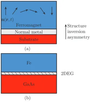
II. THE SYSTEM AND ITS ENERGY SCALES The system consists of a substrate/normal-metal/magnetic material structure, as sketched in Fig.1(a), and is characterized by various energy scales, which will now be introduced. First of all, the Fermi energyF is assumed to be much larger than any other relevant energy; that is, we are dealing with a “good metal.”

Ferromagnet Normal metal

Substrate n(r, t)

Structure inversion asymmetry

Fe

GaAs

2DEG (a)

(b)

FIG. 1. (a) A sketch of the considered structure; n(r,t) is the magnetization direction in the magnetic material, here illustrated as a N´eel domain wall. The precise nature of the magnetic layer, e.g., ferro- or ferrimagnetic insulator, is inconsequential for our treatment, although it will determine the value of the physical parameters entering the effective Hamiltonian. The same holds for the normal metal, whose thickness can be anything from a few monolayers (2D) up to tens of nanometers (3D). Electrons therein feel an effective Rashba spin-orbit field due to inversion symmetry breaking, as well as (random) spin-orbit scattering from impurities. The substrate is a generic structureless insulator, possibly the vacuum. (b) A possible experimental realization of a spin-pumping setup, where precession of the (here homogeneous) Fe magnetization drives the spin-charge dynamics of a 2D electron gas formed at the interface with GaAs.

We then assume a proximity-induced magnetization in the metallic film. The coupling between the itinerants and the localized d electrons, i.e., the induced magnetic texture, is described within thes-d model:

H_sd=_xcn(r,t)·σ

2, (1)

whereσ =(σ^x,σ^y,σ^z) denotes the vector of Pauli matrices, _xc is the ferromagnetic exchange band splitting, and n is the magnetization direction. At first sight, this model might appear questionable since we wish to study the dynamics in the nonmagnetic metallic film. However, it is known that metals like Pt and Pd can be magnetized due to the magnetic proximity effect [45–47] and that the exchange energy may be large, i.e., much larger than the disorder broadening,_xcτ/¯h1, with τ denoting the momentum relaxation time. The precise value of_xcdepends on the material properties of the magnetic and nonmagnetic layers and of the interface.

Furthermore, we assume two types of spin-orbit coupling, a Rashba-like spin-orbit term due to structure inversion asymmetry [see Fig.1(a)] and extrinsic spin-orbit coupling due to impurities. The Rashba spin-orbit coupling Hamiltonian reads

H_R = −α

¯

hσ×zˆ·p, (2)

with the Rashba parameter α estimated to be between 0.03 and 3 eV ˚A, depending on the structure and material properties of the system [48]. The associated spin-orbit splitting_so= 2αpF/¯h is taken to be small in the sense that _soτ/¯h1.

This condition is often appropriate and, in addition, useful for obtaining physically transparent equations for the spin-charge coupled dynamics. However, since typical values for the spin- orbit splitting are in the range 10⁻³, . . . ,10⁻¹ eV [26,28,29], this condition is not universally realistic. Extrinsic spin-orbit coupling with impurities is described by

H_ext= −λ²

4¯hσ×∇V(r)·p, (3) whereλis the effective Compton wavelength, whose strength is material and impurity type dependent, andV(r) is the disor- der potential. Due to the two types of spin-orbit coupling, both Dyakonov-Perel (DP) and Elliott-Yafet (EY) spin-relaxation mechanisms are present. The corresponding energies are given by

¯ h τ_DP =h¯

2mα

¯ h²

₂

D, (4)

¯ h τs =h¯

τ λpF

2¯h 4

, (5)

respectively, with the effective massm, the Fermi momentum pF, and the diffusion constant D=v²_Fτ/d, where d =2,3 represents the dimensionality. Note that the expression for

¯

h/τ_DP follows from the condition _soτ/¯h1. Dyakonov- Perel relaxation is intrinsically nonisotropic since the Rashba term (2) contains only in-plane momenta, and while its strength depends on the dimensionality of electronic motion through D, its anisotropy does not. Elliot-Yafet relaxation is, on the other hand, strongly anisotropic only in the 2D limit. Here, however, “2D” does not refer to the electronic motion, being rather determined by the ratio of the metal thicknesst_mto the spin-relaxation length: Elliott-Yafet is 2D (3D) roughly for small (large)tm in this sense. The transition is modeled by introducing a phenomenological parameter 0< ζ <1, with ζ =0↔2D, ζ =1↔3D (see Sec. III). We focus on the experimentally relevant regime 1/τ_DP 1/τs [22]. Together with the strong exchange assumption,_xcτ/¯h1 [47], this leads to the following hierarchy of energy scales:

¯ h _xcτs

β_s

h¯ _xcτ_DP

β_DP

h¯

_xcτ 1 h¯

_soτ. (6)

Equation (6) defines the spin torque parameters βs andβ_DP, which will appear repeatedly below.

The magnetization is assumed to be smooth on the Fermi wavelengthλ_Fscale, and the frequency of its time dependence is taken to be small compared to the spin-flip rate,

ωτs/¯h1, (7) applicable for the typical adiabatic pumping regime. In Sec.IV, we will in addition consider the diffusive regime,

ωτ,ql1, (8)

where q is the typical wave vector of the system inhomo- geneities andl=v_Fτ the mean free path.

III. THE KINETIC EQUATIONS

In order to describe the transport phenomena in the presence of spin-orbit coupling and a magnetic texture, we use the SU(2) formulation of the Boltzmann-like equation [38]. The Hamiltonian of the system reads

H = 1 2m

p+A^aσ^a 2

2

+e+^a(r,t)σ^a

2 +V(r)+H_ext, (9) where A^a is an SU(2) vector potential which describes the intrinsic spin-orbit coupling, is the electric potential withe= |e|, and^a is an SU(2) scalar potential. Here and throughout the paper, upper (lower) indices will indicate spin (real-space) components. A summation over repeated indices is implied.

For the system discussed in Sec.II, we have

H_sd↔ ^a(r,t)=_xcn^a(r,t), (10) H_R ↔ A^xy= −A^yx =2mα

¯

h (11)

[compare Eqs. (1) and (2)].

According to Ref. [38] and forδ-correlated (short-range) disorder, the Boltzmann equation for the distribution function f =f⁰+f·σ, with f⁰ (f) denoting the particle (spin) distribution function, reads

∂˜_tf + p

m·∇˜rf +1

2{F,∇pf} = −1

τ(f − f )+I_EY[f], (12) where· · · denotes the angular average with respect to the momentum. The covariant time (spatial) derivative ˜∂_t( ˜∇r) and the generalized forceFare given by

∂˜t =∂t−i

¯ h

^aσ^a

2 ,· , (13)

∇˜r=∇r+i

¯ h

A^aσ^a

2 ,· , (14)

F = −eE−

E+ p m×B

a

σ^a

2 , (15)

and

Ei^a = −∇i^a−1

¯

hε^abcbA^ci, (16) B^ai = −1

2¯hεij kε^abcA^bjA^ck, (17) with∇i denoting the ith component of ∇r. The dot within the commutator in Eqs. (13) and (14) is a placeholder for the object on which the covariant derivative acts. Using Eqs. (10) and (11), theith component of the generalized force reads

Fi = −eE_i+_xc( ˜∇in)·σ

2 −2mα²

¯

h³ ε_{ij z}p_jσ^z. (18)

FIG. 2. Impurity-averaged self-energy which determines the Elliott-Yafet collision operator. The boxed crosses, the dashed line, and the arrowed double line represent spin-orbit coupling, impurity correlations, and the Green’s function in Keldysh space, respectively.

The ith component of the (3D) covariant derivative ˜∇i is defined as

∇˜i =∇i+[ai]_×, (19) where we have introduced the notation for an antisymmetric matrix [v]_× with its components defined by ([v]_×)^ab=

−ε^abcv^c. This definition corresponds to a cross product in the

sense that [v]_×b=v×bfor an arbitrary vectorb. The vector ai is defined asai =2mα/¯h²(−δ_iy,δ_ix,0). Analogously, from now on we use the “3D covariant time derivative,” defined as

∂˜t =∂t+_xc

¯

h [n]_×. (20) The quantityI_EY on the right-hand side (rhs) of Eq. (12) is the Elliott-Yafet collision operator, representing spin-flip processes. It follows from the impurity-averaged self-energy as depicted in Fig. 2 and is substantially modified in the presence of intrinsic spin-orbit coupling and magnetic textures.

The corrections are obtained via a first-order SU(2) shift (see AppendixA), which yields the following generalized collision integral:

I_EY=I_EY⁰ +δI_EY +δI_EY^A , (21) where

I_EY⁰ = − 1 2N0τ

λp 2¯h

4

dpδ(p−p)[(fp+fp)]·σ, (22) δI_EY = mp²

N₀τ λ

2¯h 4

dpδ(p−p)()·

f_p⁰σ+fp−

1+p∂_p

f_p⁰σ−fp

, (23)

δI_EY^A = 1 N₀τ

λ 2¯h

₄

dpδ(p−_p)A^a·Lp,p

σ^a

f_p⁰−f_p⁰

+

f_p^a+f_p^a

, (24)

with=_xcn,dp≡d^dp/(2πh)¯ ^d,Lp,p =(p²+p·p)p− (p²+p·p)p, N₀ being the density of states per volume and spin, and =diag(1,1,ζ). The latter takes into ac- count the anisotropy of spin-flip processes, as discussed above, and hence depends on the thickness tm of the nor- mal metal. Clearly, 0ζ 1, with ζ =0 representing the limit that the normal metal is a 2D gas, i.e., for small t_m, whereas one may assume ζ =1 when t_m> _s, where s is the spin-relaxation length of the normal metal. We emphasize that Eqs. (23) and (24) are valid for arbitrary spin-orbit fields, not only Rashba coupling, and magnetic textures.

Expressions (23) and (24) are “first order” in the SU(2) fields, provided we take the spin distribution function f to be “zero order.” However, as discussed in the next section in connection with Eq. (30), f contains a local- equilibrium part feq, which formally is also first order.

Thus, in order to treat relaxation due to the EY collision operator consistently, it becomes necessary to include also a specific second-order correction in the SU(2) shift, which is given by

δI_EY^A, = − 1 4τ

λ 2¯h

₄

·Aip_ip²∂_p

_p∂_pf_eq⁰

, (25) where f_eq⁰ is the Fermi function. As a consequence, only the nonequilibrium part of the spin density δs will enter the effective force, Eq. (48). An even more de- tailed investigation of the EY collision operator is well underway [49].

IV. SPIN-CHARGE COUPLED DYNAMICS

Here, we present the coupled equations for the electron density, the electron current, the spin density, and the spin current, respectively defined as follows [50]:

n=2

dpf⁰, (26) j_i =2

dppi

mf⁰, (27)

s=

dp f, (28)

j_i^a =

dppi

mf^a. (29)

We focus first on the spin sector (Sec.IV A) and second on the charge sector (Sec.IV B) and third discuss the interpretation of the different contributions to the effective force (Sec.IV C).

A. Spin sector

In order to study the spin sector, we multiply the Boltzmann equation by the Pauli vectorσ and perform the trace. Before doing so, it is convenient to split the spin distribution function fas

f=feq+δf, (30)

withf_eq=(−∂_pf_eq⁰)(_xc/2)n, wheref_eq⁰ is the Fermi function.

This is motivated by the form of the spin density

s=s_eq+δs, (31)

where s_eq=(N_0xc/2)n is the equilibrium part of swhich adiabatically follows the magnetization. The dynamics of the itinerant electrons, which is typically much faster than the magnetization dynamics, leads to the nonequilibrium contributionδs.

We trace over the spin sector and obtain the following 3×3 matrix equation:

Mδf=Nδf +S, (32) with

M=1+ τ 2τs

+τ∂˜t+τp_i

m∇˜i, (33) N=1− τ

2τs

, (34)

S=

∂_pf_eq⁰τ _xc

2 n.˙ (35)

Note that we have neglected small deviations off⁰ from its angular average,f⁰ f⁰ , since these are at least first order in the electric fieldEor the magnetic texture, i.e.,∇inor ˙n.

Furthermore, we assumef⁰ f_eq⁰.

By an integration of the spin sector over the momentum we obtain

∂˜tδs+∇˜iji= −1

τ_sδs−N_0xc

2 n.˙ (36)

Next, we consider the quasiadiabatic limit, τs∂tδsδs, as well as τs∂tδsζ δs. We are then able to solve for the nonequilibrium spin density:

δs=(δs)_n+(δs)j_s, (37) where

(δs)_n= −N_0xcτs

2

+β_s⁻¹[n]_×−1

n˙ (38) denotes the part ofδs which is associated directly with the magnetization and

(δs)j_s = −τs

+β_s⁻¹[n]_×−1∇˜iji (39) the part which is associated with the spin current. In general the spin current itself depends on the spin density, which has to be kept in mind when solving for the spin density from Eq. (36).

The split in Eq. (37) is found to be technically convenient.

In the following, we shall calculate the spin current in the diffusive regime. Our approach is to rewrite the matrixMin Eq. (32) as follows:

M=(1+ξ)M, (40) where

M=

1+_xcτ

¯ h [n]_×

(41) and

ξ = τ

2τs

+τ ∂t+τp_i m∇˜i

M⁻¹. (42) In the diffusive regime we can approximate (1+ξ)⁻¹1−ξ and rewrite Eq. (32) as

δf=M⁻¹(1−ξ)

Nδf +S

. (43)

Effective force Fi= (Fi)_s+ (Fi)_js Spin density

δs= (δs)_n+ (δs)js

Spin current ji= (ji)_n+ (ji)_s Magnetization

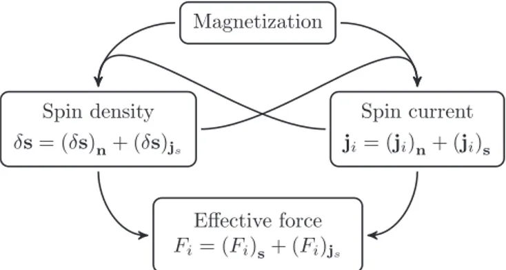
FIG. 3. Scheme of the various contributions to the effective force.

By multiplying the latter equation byp_i/mand integrating over the momentum, we obtain the spin current:

ji =(ji)_n+(ji)_s, (44) where

(ji)n=τ

2DN_0xcM⁻¹∇˜iM⁻¹n˙ (45) denotes the part arising directly from the magnetization and

(ji)s= −DM⁻¹∇˜iM⁻¹δs (46) the part of the spin current which has its source in the spin density.

B. Charge sector

For the charge sector, we trace over the Boltzmann equation (12), multiply byp_i, and integrate over the momentum, with the following result:

(1+τ ∂_t)ji+D∇in= −nμE_i+τ N_0xc

m F_i, (47) where μ=eτ/m is the electron mobility and nμ=σD/e, withσD being the Drude conductivity. The effective forceFi

combines the contributions of the nonequilibrium part of the spin density and the spin current.

A scheme of the various contributions to the effective force is depicted in Fig.3. We splitFi=(Fi)_s+(Fi)j_sinto two terms which represent the contribution of the spin density (Fi)sand the direct contribution of the spin current (Fi)j_s. According to this split, it is clear that (Fi)sis associated with the SGE, and (Fi)js is associated with the ISHE. The two contributions to the effective force explicitly read

(Fi)s= 1 N₀

∇˜in

·δs+2mα

¯

h² βs(ˆz×δs)i , (48) (Fi)j_s = 1

DN₀

β_DP j^z׈z

i+ τ τs

nζ ·ji , (49) withnζ =n. With respect to the second term on the rhs of Eq. (48), compare it to the discussion in connection with Eq. (25).

We further divide (Fi)sinto contributions arising from (δs)n

and (δs)js:

(Fi)s=(Fi)s,n+(Fi)s,js, (50)

where (Fi)s,n and (Fi)s,js have the same form as (Fi)s in Eq. (48), but with δs being replaced by (δs)n and (δs)js, respectively. Analogously, we define

(Fi)j_s =(Fi)j_s,n+(Fi)j_s,s, (51) with (Fi)js,n and (Fi)js,s having the same form as (Fi)js

in Eq. (49), but with ji being replaced by (ji)n and (ji)s, respectively. The idea behind this separation is to express the effective force in terms of the drive ˙nand the spin current, with the subscripts indicating the respective origins.

1. The contribution(Fi)_s,n

The spin density related directly to the dynamical magne- tization [see Eq. (38)] is explicitly given by

(δs)_n=hN¯ ₀ 2

1

n²_ζ[nζ ×n˙−β_sζ ⁻¹n].˙ (52) We insert Eq. (52) into Eq. (48) and find

(Fi)s,n=h¯ 2

1 n²_ζ

(∇in)·

nζ ×n˙−βsζ ⁻¹n˙ +2mα

¯

h² [(n·nζ)ˆz×n˙

+β_sˆz×(nζ ×n˙+ζn×⁻¹n)]˙ i

. (53) Assumingζ =1 (i.e.,t_ms), the last equation reduces to Eq. (11) in Ref. [51] (see also Refs. [35,52–56]). Recall thatζ describes the anisotropy of spin-flip relaxation and thatζ =1 corresponds to the isotropic case. As far as we know, this is the first time that such anisotropy (ζ <1) is explicitly taken into account. However, experiments on thin films typically deal with samples on the scale of a few nanometers; hence, it is appropriate to include this effect.

2. The contributions(Fi)s,j_sand(Fi)j_s,n(homogeneous case) For the sake of simplicity and since we are mostly interested in the competition between the SGE and the (in-plane) ISHE, we shall focus here on the Rashba contribution; that is, we consider ˜∇i ≈[ai]_×in Eqs. (39) and (48), which corresponds to a spatially homogeneous situation. Neglecting terms∼β_s² and smaller for the spin-density-dependent contribution, we find

(Fi)s,j_s = 1 DN₀

1 n²_ζβ_DP

(n·nζ)[ˆz×(j^z)n]i

+2

a=x,y

nz

j_a^a

n−na

j_a^z

n

(ˆz×n)i

. (54) Adding the contribution by (ji)n[Eq. (49) withji →(ji)n], we obtain

(Fi)s,j_s+(Fi)j_s,n= 1 DN₀

β_DPζ(1−ζ)n²_z

n²_ζ [ˆz×(j^z)n]i+2βDP

×

a=x,y

n_z j_a^a

n−n_a j_a^z

n

(ˆz×n)i

+ τ τs

nζ ·(ji)_n. (55)

Note that (Fi)js,n features a direct contribution due to the driving source, i.e., ˙n, whereas (Fi)js,s contributes more indirectly throughδs. Apparently, Eq. (55) yields a nontrivial interplay between the two “origins” [spin density versus spin current; see Eqs. (50) and (51)] since the first term on the rhs of Eq. (49) is canceled to some extent by the first term on the rhs of Eq. (54). This demonstrates once more that the interplay between SGE and ISHE is nontrivial.

C. Discussion: Effective forces

We emphasize that expressions (48) and (49), obtained by properly integrating the kinetic equation, have general validity.

Before going into the details of the spin-pumping configuration (Sec. V), we comment on the relation of these equations to previous results. First, neglecting the Rashba contribution in the first term on the rhs of Eq. (48), i.e., ˜∇in→∇in, considering the isotropic case (ζ =1), and taking into account that

δs=hN¯ ₀

2 [n×n˙−βsn]˙ (56) in this limit, this force term agrees with the result given in Ref. [35]. Second, including the Rashba contribution but neglecting the spin current contribution toδs[see Eq. (39)]

and again forζ =1, Eq. (48) reduces to Eq. (11) in Ref. [51].

Third, the first term on the rhs of Eq. (49), which is due to Rashba spin-orbit coupling, is related to the ISHE: a charge current in thex−y plane is generated by a spin current (in that plane) polarized in thezdirection, with the charge current direction being perpendicular to the spin current direction,

∼j^z×zˆ(cf. Ref. [6]).

Note, however, that the various terms are not independent of each other. In particular, spin density and spin current are closely related, as already pointed out in Ref. [57], due to the interplay of Rashba coupling and EY relaxation. This is apparent from Eq. (36), which for time-independent and spatially homogeneous situations reads

_xc

¯

h n×δs+ai×ji= −1

τ_sδs. (57) Taking this equation into account, it is possible to relate the total effective force derived here to the one discussed in Ref. [23] [see Eq. (12) therein]. First, consider the limit _xc→0, which leaves only the second term in (48) and the first term in (49). The latter is readily identified with the “Hall-like” force [23]; however, using Eq. (57), we find that Eq. (48), which results from the EY collision operator [Eq. (24)], gives an identical contribution; thus, our result appears to be larger by a factor of 2. Further differences become apparent for finite_xc.

Last but not least, the second term on the rhs of Eq. (49) is denoted the “inverse-spin-filter” term, as it describes a force arising from a spin current which is polarized parallel to the magnetization (roughly speaking), with its strength being

∼τ_s⁻¹. To the best of our knowledge, such a term has not been explicitly considered before. However, it can be related to the anomalous Hall effect: imagine that an electric field in the x direction creates a spin current via the spin Hall effect (in they direction, polarized in thezdirection). This spin current leads, via the inverse-spin-filter term, to a charge

current in they direction. Note that a nonzeroζ is required for this argumentation to be valid. In this context, see also the discussions given in Refs. [47,58].

V. SPIN-PUMPING CONFIGURATION

In this section we consider the magnetization dynamics to be fixed, namely, as a precession with a cone angle θ and angular frequencyωabout an axis fixed by an external static and homogeneous magnetic field [59]. The magnetization direction is parametrized as follows:

n(t)=R_φ

⎛

⎝ n₀ δn_y(t) δn_z(t)

⎞

⎠=R_φ

⎛

⎝ cosθ sinθcosωt

sinθsinωt

⎞

⎠, (58)

withRφbeing a rotation matrix around thezaxis, Rφ=

⎛

⎝cosφ −sinφ 0 sinφ cosφ 0

0 0 1

⎞

⎠, (59)

where φ is the angle between the x axis and the cone axis (see Fig.4).

Furthermore, we assume open-circuit conditions in thex andydirections in order to determine the electric field along these directions. Since the magnetization is homogeneous, we expect the particle current to be homogeneous as well, and due to the open-circuit condition we have jx,y=0 in the whole sample. From Eq. (47) we find

σDEx,y= eτ N_0xc

m Fx,y. (60) According to Ref. [57], the spin Hall conductivity can be expressed as [60]σ^sH=e¯hτ N₀/2mτs (forτ_s τ_DP); hence, we may rewrite Eq. (60) as

eEx,y= 2θ^sH βs

Fx,y, (61) where θ^sH=eσ^sH/σ_D is the spin Hall angle. In order of magnitude, θ^sH∼h/¯ _Fτ_s. Our focus in the following is on the dc contribution to the electric field; thus, we will average Eq. (61) with respect to time.

n

(a) (b)

z (t) yx

j_y E_x

FIG. 4. (a) The studied configuration, i.e., a metallic film on top of a magnetic material (shown in blue). (b) Sketch of the conical precession of the magnetization, defining the relevant angles θ andφ.

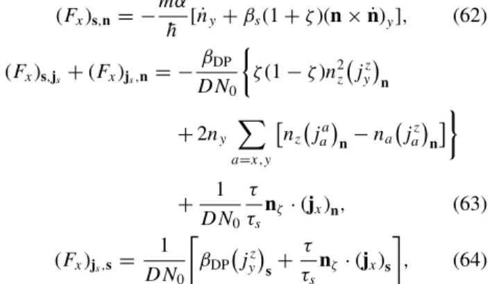
Let us now explicitly consider the x component of the effective force. According to Eqs. (53) and (55), as well as Eq. (49) withji →(ji)s, it is the sum of the following three contributions:

(Fx)s,n= −mα

¯

h [ ˙n_y+β_s(1+ζ)(n×n)˙ _y], (62) (Fx)s,j_s+(Fx)j_s,n= −β_DP

DN₀

ζ(1−ζ)n²_z j_y^z

n

+2ny

a=x,y

nz

j_a^a

n−na

j_a^z

n

+ 1 DN₀

τ τs

nζ ·(jx)_n, (63) (Fx)js,s = 1

DN₀

β_DP j_y^z

s+ τ τs

nζ·(jx)_s , (64) where, in order to derive Eqs. (62) and (63), we approximated n²_ζ 1 andnζ ·n1 since the cone angleθis usually small [8]. For this reason, we shall also allow only terms up to sin²θ when performing the time average; hence, we neglect terms of ordern²_z since the time average would lead to∼sin⁴θterms.

We realize that the first term on the rhs of Eq. (63), which has its origin in the interplay of the spin density and the spin current, is negligible.

We rewrite Eqs. (62)–(64) in order to elucidate the different effects:

F_x^(A) = β_DP DN₀

j_y^z

s, (65)

F_x^(B) = −mα

¯

h [ ˙n_y+β_s(1+ζ)(n×n)˙ _y]

−2β_DP DN₀ny

a=x,y

nz

j_a^a

n−na

j_a^z

n

, (66)

F_x^(C) = 1 DN₀

τ

τ_snζ ·jx, (67) whereF_x^(A)can be related to the ISHE andF_x^(B)can be related to the SGE. The last term, F_x^(C), describes the buildup of an effective force (or electric field) due to the spin current polarized parallel to the magnetization [61] and is denoted the inverse-spin-filter term, as discussed in Sec.IV B.

Analogously, we obtain for theycomponent F_y^(A) = −β_DP

DN₀ j_x^z

s, (68)

F_y^(B) =mα

¯ h

˙

n_x+β_s(1+ζ)(n×n)˙ x

+2β_DP DN₀nx

a=x,y

nz

j_a^a

n−na

j_a^z

n

, (69)

F_y^(C) = 1 DN₀

τ τs

nζ ·jy. (70) In the following sections, we consider a narrow wire (see Fig. 5) and the electric field that will be measured in longitudinal and orthogonal measurements. We assume that the wire is “narrow” such that the width of the wire is smaller than the spin diffusion length_s =√

Dτ_s. For such a

FIG. 5. Bottom: top view of the setup; the length is denotedlx, and the width is denotedly(l_y lx). Top: qualitative plot of the dc electric fields,eEx tandeEy t, for longitudinal (left) and orthogonal (right) measurements. In both cases we setζ=0.

configuration, the spin current contribution polarized parallel to the magnetization and flowing parallel to the narrow edge vanishes (see AppendixB).

A. Longitudinal measurement

Let us consider a narrow wire as depicted in Fig.5. For such a sample we find a homogeneous spin current flowing in the x direction which, in particular, has a contribution polarized alongn, giving rise to the force in Eq. (67) when performing a longitudinal measurement. We perform the time average of Eqs. (65)–(67), insert the results into Eq. (61), and obtain the following dc electric fields:

E^(A)_x

t ∼β_DPθ^sHFα

e θ^sHFα

e , (71) E_x^(B)

t = −2θ^sHFα

e (1+ζ) sinφsin²θ, (72) E_x^(C)

t = −θ^sHFα

e (1−ζ) sinφsin²θ, (73) withFα≡αωm/¯h. We realize that the ISHE (A) term plays only a minor role in the total electric field,Ex t = E^(A)_x + E_x^(B)+E_x^(C) _t. Note that for ζ 0 the inverse-spin-filter contribution is of the same order of magnitude as the SGE term, whereas it vanishes forζ =1.

B. Orthogonal measurement

In the case of an orthogonal measurement (see Fig.5, right), the contribution given in Eq. (70) vanishes since the spin current jy lacks a contribution parallel to the magnetization (ly s). For the dc electric field along they direction, we find

E_y^(A)

t ∼β_DPθ^sHFα

e θ^sHFα

e , (74) E_y^(B)

t = −2θ^sHFα

e (1+ζ) cosφsin²θ, (75) E^(C)_y

t =0, (76)

leaving only the SGE term to contribute to the total dc electric field.

C. Discussion

Comparing the results for the longitudinal and orthogonal measurements, we see that the signal can be up to 1.5 times larger in the longitudinal measurement (forζ =0; see Fig.5).

For a 2D electron gas one should thus be able to probe a Rashba-induced SGE and, by comparing samples of different thicknesses, to additionally obtain estimates ofαandζ.

Recent articles [3,8,9,62] discussed spin pumping and the induced ISHE on the basis of a spin currentjz which flows perpendicular to the interface, i.e., in the z direction into the normal-metal film. This is significantly different from the situation we are discussing here (jz=0). Nevertheless, the electric field estimated in such a way [8] shows the same angular dependence of the magnetization as our result:

Ref. [8]: Ex ∼Fg↑↓sinφsin²θ, (77) Eq. (72): E_x∼F_αsinφsin²θ. (78) Comparing the relevant forces,F_g↑↓ =e²ωg^↑↓/(4σD) andF_α, for reasonable parameter values, g^↑↓≈2.1×10¹⁹m⁻² and σD≈2.4×10⁶⁻¹m⁻¹, for a Pt film [8], we find the forces to be of the same order of magnitude forα≈0.3 eV ˚A. Thus, we conclude that the SGE contribution and the inverse-spin-filter effects due to Rashba-induced spin currents and spin density, as discussed here, should both be taken into account when interpreting experiments.

VI. CONCLUSIONS

We have studied the spin-charge coupled dynamics in a magnetized thin metallic film with Rashba spin-orbit coupling.

In particular, we have considered a generalized Elliott-Yafet collision integral, valid for arbitrary spin-orbit fields and magnetic textures, and taken into account anisotropic spin-flip processes. Significant modifications of the kinetic equations describing spin and charge transport have been found. The effective force acting on the charge carriers in the presence of spin-orbit coupling has been derived in a very general form and has been evaluated in detail for the case of a time-dependent texture. For a narrow wire in the typical spin-pumping configuration an in-plane electric field is generated, for which the spin-galvanic effect is crucial, while the (in-plane) spin Hall effect turns out to be negligible. However, an additional contribution of similar strength from an inverse-spin-filter effect is found to be relevant for a longitudinal measurement, while it vanishes for an orthogonal measurement. This suggests the possibility of determining the strength of the spin-galvanic effect and the spin-orbit coupling parameter, Rashba in our specific scenario, by performing both measurements on the same sample.

ACKNOWLEDGMENTS

We acknowledge stimulating discussions with C. Back, L. Chen, M. Decker, and R. Raimondi. We especially are indebted to L. Chen for helpful comments on the manuscript.

We acknowledge financial support from the German Research Foundation (DFG) through TRR 80 (U.E., S.T.) and SFB 689 (C.G.).

APPENDIX A: THE ELLIOTT-YAFET COLLISION OPERATOR

In this appendix we follow the procedure outlined in Ref. [38]. We start by deriving the Elliott-Yafet collision operator within first order in the SU(2) fields from the microscopic Green’s function G and the Elliott-Yafet self- energy _EY (diagrammatically depicted in Fig. 2) in the two-dimensional case and comment on the three-dimensional case at the end.

The Elliott-Yafet collision operator is given by I_EY= − 1

4π¯h

dL˜^K, (A1) withL=[_EY,G]. The superscriptKrepresents the Keldysh component, and the tilde indicates the SU(2) shift; clearly,

L˜ =[ ˜_EY,G]. In first order, we have˜ L˜ ≈L−¹₂

Aμ,∂_p^μL

, (A2)

with the four-potentialAμ=(−,A) and∂p^μ=(∂,∇p). We recall that the components of the four-potential are SU(2) gauge fields, i.e., =^aσ^a/2 and A=A^aσ^a/2. In order to derive the explicit expression for the collision operator, we need in the first step the impurity-averaged and SU(2)-shifted self-energy (compare Fig.2), which reads

˜_EY=˜_EY⁰ +δ˜_EY +δ˜^A_EY, (A3) with

˜⁰_EY=C

d²p

(2πh)¯ ²σ^zG(p˜ )σ^z(p×p)²_z, (A4) δ˜_EY = C

2∂

d²p (2πh)¯ ²

σ^z

^aσ^a

2 ,G(p˜ )

σ^z−

^aσ^a

2 ,σ^zG(p˜ )σ^z

(p×p)²_z, (A5)

δ˜_EY^A = C 2

d²p (2πh)¯ ²

σ^z

A^aσ^a

2 ,[∇pG(p˜ )]

σ^z−

A^aσ^a

2 ,σ^zG(p˜ )σ^z

∇p

(p×p)²_z, (A6)

whereC=(2π τh¯³N₀)⁻¹(λ/2)⁴. For the Green’s functions we have

G˜^K =( ˜G^R−G˜^A)(1−2f), (A7) where f =f⁰+f·σ denotes the distribution function 2×2 matrix; furthermore,

G˜^R−G˜^A= −2π iδ(−p). (A8) Note that the SU(2)-shifted retarded and advanced Green’s functions are diagonal in spin. Inserting ˜Linto Eq. (A1) and using Eqs. (A4)–(A8) lead to the collision operators as given in Eqs. (22)–(24) forζ =0, corresponding to the 2D case.

When we consider the bulk 3D case, we have the following replacement:

σ^z· · ·σ^z(p×p)²_z→σ^a· · ·σ^b(p×p)a(p×p)b (A9) within the integrals in Eqs. (A4)–(A6), respectively. Then we obtain, using the same procedure as outlined in Sec. I, Eqs. (22)–(24) for ζ =1, except for a small numerical difference related to the angular average in 2D versus 3D.

In order to describe the anisotropy in the intermediate regime, we insert the matrix=diag(1,1,ζ), with 0ζ 1 [see Eqs. (22) and (23)].

APPENDIX B: NARROW WIRES

Here, we show that the contribution which is polarized parallel to the magnetization of the spin current flowing in the narrow direction vanishes in the homogeneous case. We consider a narrow wire along thexdirection, i.e.,lysand lx s, and an open-circuit condition, jy(y =0)=jy(y= ly)=0. For the sake of simplicity we put ζ =1. Since the system is homogeneous, we assume that the spin current

flowing in thexdirection is homogeneous as well and given by Eqs. (44)–(46) with ˜∇x →[ax]_×. According to Eqs. (37)–(39) the spin density can be expressed as

δs(y)=δs0−τsM_s⁻¹∇˜yjy(y), (B1) with

δs0=(δs)n−τsM_s⁻¹[ax]_×jx. (B2) In addition, M_s =M(τ →τ_s), where M [see Eq. (41)] is explicitly given by

M=1+_xcτ

¯

h [n]_×=β_τ⁻¹

⎛

⎝ βτ −nz ny

nz βτ −nx

−n_y n_x β_τ

⎞

⎠, (B3)

whereβ_τ =h/¯ _xcτ. The spin current flowing in theydirection is given by Eqs. (44)–(46):

jy(y)=DM⁻¹∇˜yM⁻¹

N₀β_τ⁻¹n˙−δs(y)

. (B4) We insert Eq. (B1) into Eq. (B4) and obtain approximately ( ˜∇yjy ∇yjy) the following differential equation:

1−²_sM_s⁻¹M⁻²∇y²

jy(y)=j_y,0, (B5) where the rhs, which is spatially constant, is given by

j_y,0=DM⁻¹[ay]_×M⁻¹

N₀β_τ⁻¹n˙−δs₀

. (B6) It is apparent thatjy,0 is a particular solution of Eq. (B5).

In order to determine the complete solutionjy =jy,h+jy,0, we have to add the solution of the homogeneous differential equation, which can be written as follows:

MsM²−²_s∇y²

jy,h(y)=0. (B7)