Spin Current Induced Control of Magnetization Dynamics

Spin Current Induced Control of Magnetization Dynamics

Dissertation

zur Erlangung des Doktorgrades der Naturwissenschaften (Dr. rer. nat.)

der Fakultät für Physik der Universität Regensburg

vorgelegt von

Martin Maria Decker

aus München

im Jahr 2017

Promotionsgesuch eingereicht am: 29.10.2017

Die Arbeit wurde angeleitet von: Prof. Dr. Christian Back Prüfungsausschuss: Vorsitzender:

1. Gutachter:

2. Gutachter:

weiterer Prüfer:

Prof. Dr. Karsten Rincke

Prof. Dr. Christian Back

Prof. Dr. Jaroslav Fabian

PD Dr. Alfred (Jay) Weymouth

Der Termin des Promotionskolloquiums: 08.02.2018

Contents

Introduction 1

I. Micromagnetism and Spin Orbit Torques: Theoretical Framework 5

1. Magnetization Dynamics I: Energy Terms and Equation of Motion 7

1.1. Micromagnetism . . . . 7

1.2. Energy Contributions . . . . 8

1.2.1. Exchange interaction . . . . 9

1.2.2. Dzyaloshinskii-Moriya interaction . . . . 9

1.2.3. Magnetostatic energy . . . . 10

1.2.4. Crystalline anisotropy . . . . 12

1.2.5. Interface anisotropy . . . . 13

1.3. Landau-Lifshitz-Gilbert Equation . . . . 15

2. Spin Orbit Torques (SOTs) in Metallic Multilayers 19 2.1. Spin and Charge Currents . . . . 19

2.1.1. Drift diffusion equation for charge . . . . 20

2.1.2. Drift diffusion equation for spin . . . . 20

2.1.3. Drift diffusion in ferromagnets . . . . 21

2.2. Spin Hall Effect (SHE) . . . . 22

2.3. Rashba-Edelstein Effect . . . . 26

2.4. Spin Transport Across a Normal Metal/Ferromagnet Interface . . . . 29

2.5. SHE Induced Torques . . . . 32

2.5.1. Drift diffusion model for SHE induced SOTs . . . . 33

2.5.2. Data evaluation of direct SHE experiments . . . . 35

3. Magnetization Dynamics II: Theory of Ferromagnetic Resonance (FMR) 37

Contents

II. Experimental Quantification of Spin Orbit Torques: Comparison of Di- rect (SHE) and Inverse (ISHE) Spin Hall Measurements in Pt/Py Bi-

layers 45

1. Review of Experimental Techniques 51

2. Coplanar Waveguide Based FMR: Creation of Static and Dynamic Fields 55

2.1. Static Field . . . . 55

2.2. Creation of the Driving Field . . . . 56

2.2.1. Coplanar waveguides . . . . 56

2.2.2. Oersted fields due to induced currents . . . . 59

3. Absorption FMR 61 3.1. Theoretical Considerations . . . . 61

3.2. Experimental Realization . . . . 62

4. Quantification of SOTs by Modulation of Damping (MOD) 65 4.1. Theoretical Aspects of MOD . . . . 65

4.2. Time and Space Resolved FMR . . . . 66

4.2.1. Magneto-Optical Kerr effect (MOKE) . . . . 66

4.2.2. Time resolved MOKE . . . . 68

4.2.3. Sample geometry for MOD experiments . . . . 72

5. Quantification of the SHE by the Spin Pumping Driven ISHE 75 5.1. Spin Pumping (SP) . . . . 75

5.2. SP Driven ISHE . . . . 78

5.2.1. Origin and form of the ISHE voltage . . . . 78

5.2.2. Rectified voltage due to anisotropic magnetoresistance (AMR) . . . 80

5.2.3. Angular dependence of AMR and ISHE voltage . . . . 81

5.3. Experimental Access to ISHE . . . . 85

6. Standing Spin Waves in Magnetic Microstripes 87 6.1. Longitudinally Magnetized Stripes . . . . 90

6.2. Transversely Magnetized Stripes . . . . 92

6.3. Implication for SOT Measurements . . . . 95

7. Boltzmann Transport in Thin Metallic Layer Systems 97 7.1. Drude Theory . . . . 98

7.2. Fuchs-Sondheimer Model . . . . 99

7.3. Mayadas-Shatzkes Model . . . 103

7.4. Current Density Distribution in Bilayers . . . 105

II

Contents

8. Growth of the Pt/Py Bilayer Series 109

9. Experimental Characterization of Magnetic and Electric Properties 113

9.1. Magnetic Properties I: Saturation Magnetization . . . 113

9.2. Magnetic Properties II: Full Film FMR . . . 114

9.3. Experimental Results of SP . . . 116

9.4. Electrical Conductivity . . . 117

10. ISHE: Micromagnetic Simulations and Experimental Results 125 10.1. Micromagnetic Simulations . . . 125

10.1.1. Implementation of the problem to Mumax . . . 126

10.1.2. Evaluation process of simulation data . . . 127

10.1.3. Simulation results . . . 129

10.2. Experiment: Angular Dependency . . . 133

10.3. Experiment: Pure ISHE . . . 135

11. MOD: Experimental Results 139 11.1. Experimental Requirements . . . 139

11.2. Experimental Results . . . 140

11.2.1. Field-like torque . . . 141

11.2.2. Damping-like torque . . . 142

12. Discussion of SP, ISHE and MOD Results 147 13. Summary 153 III. Time Resolved Measurements of the Spin Orbit Torque Induced Mag- netization Reversal in Pt/Co Elements 155 1. SOT Induced Switching of Perpendicularly Magnetized Elements 159 2. Sample Structure and Experimental Setup 163 2.1. Layer Sequence and Sample Design . . . 163

2.2. Experimental Setup . . . 165

3. Experimental Results 169 3.1. Time Traces of Magnetization Reversal . . . 169

3.2. Time Resolved Imaging of Magnetization Reversal . . . 171

Contents

4. Computational Analysis of the Switching Process 173 4.1. Numerical Solution of the Macrospin Model . . . 173 4.2. Micromagnetic Simulations . . . 174

5. Summary 179

IV. Appendix 181

A. Bootstrap Error Calculation 183

B. Derivation of the Dynamic Susceptibility 185

C. Static Equilibrium Change 191

Bibliography 193

List of Publications 215

Acknowledgement 217

IV

Introduction

Over the last 30 years, starting with the discovery of the giant magnetoresistive effect in 1988 [Bai88; Bin89], the idea of using the spin degree of freedom for data processing emerged and developed under the name “spintronics” [Wol01]. One branch of spintronics is dedicated to the development of new data storage devices which allow for high infor- mation densities, fast access times, low power consumption and non-volatility. A promi- nent candidate to fulfill these requirements is magnetic random access memory (MRAM) [Cha07]. Current technology uses direct current induced switching as writing mechanism and the tunneling magneto-resistance as read-out process, the so-called spin transfer torque MRAM (ST-MRAM)

. A ST-MRAM device consists of two magnetic layers separated by an oxide tunnel barrier. One of these layers is thick and pinned into a certain direction, thus called fixed layer. The second, free layer can be switched by applying a current pulse from the fixed to the free layer across the tunnel barrier. Since the current is spin polarized with polarization direction given by the fixed layer, angular momentum is transferred from the fixed to the free layer and enables switching of the free layer if the current is large enough [Cha07]. Unfortunately, the writing current across the tunnel barrier leads to its degradation and therefore is the Achilles’ heel of this technology [And14]. Thus, a way to efficiently manipulate the magnetization electrically has still to be established.

In recent years, the spin Hall effect (SHE) [Dya71b] in normal metals with strong spin orbit coupling such as Pt and Ta has been discovered and used to control the dynamics of adjacent FM layers [And08; Liu11; Dem11a; Dem11b]. The SHE converts a charge current in the NM into a transverse spin current that is absorbed by the FM and thus angular momentum is transferred from the NM to the FM. The conversion efficiency is described by the so-called spin Hall angle (SHA) θ

which connects charge current density j

and spin current density j

via j

=

θ

j

. With respect to magnetization dynamics, the SHE primarily exerts a torque of the form T

∝ m × ( m × σ

), with the unit vector of the magnetization m and the polarization direction of the injected spin current created by the SHE σ

. This torque, in certain situations, influences the effective damping of the FM and is therefore called “damping-like torque”.

While studying magnetization dynamics under the application of in-plane (ip) currents, a second effect has been discovered in metallic bilayers: in experiments concerning current

1See the manufacturer homepage: https://www.everspin.com/spin-torque-mram-technology, date:

01.12.2017

Introduction

driven domain wall movement in Pt/Co wires, a torque of the form T ∝ m × σ

, with the unit vector σ

perpendicular to both current and Pt/Co interface normal has been detected. Torques of this form are called “field-like” and from symmetry considerations the physical origin has been attributed to the so-called Rashba effect

[Mir10a].

In metallic heterostructures with ultrathin (< 1 nm) FM layers, both damping- and field- like torques have subsequently been found to appear with comparable strength. Due to the fact that the physical origin of current induced torques lies in spin orbit coupling, the term “spin orbit torque” is used as a general name without relating a measured torque to any certain physical effect (like SHE or Rashba effect) [Gar13].

Finally, the possibility of switching the magnetization of microstructured NM/FM ele- ments using ip currents has been demonstrated [Mir11; Liu12a; Liu12b]. These findings promise a transfer of technology in the writing process of MRAM cells from passing the current across a delicate tunneling barrier to passing the current through an underlying NM layer, thereby solving the above-mentioned endurance problem.

However, the physical processes incorporated in SOT induced magnetization reversal are not yet fully understood, hindering an efficient engineering towards applications. The lack of understanding is present at two levels: A) the actual dynamics of the switching process itself is unknown and completely different possible scenarios have been proposed for current induced magnetization reversal. Therefore the magnetization reversal process is hard to model, even if the strength of both field- and damping-like torques are known for a given device. B) the physical origin of the SOTs, and therefore the way to systematically increase the SOT efficiency remains unclear. There is an ongoing debate whether SHE or Rashba effect are the primary cause of the measured torques. In addition, the role of the NM/FM and FM/oxide interfaces is not yet fully understood. Part of the confusion in this field stems from the lack of using a consistent model to evaluate experimental data such that experimental results cannot easily be compared to each other.

This thesis addresses both of the above-mentioned points: One part is dedicated to the comparison of different SOT measurement techniques, focusing on the question whether the measured data can be understood within a common drift diffusion model. The second part deals with the dynamics of current induced magnetization reversal and, for the first time, presents a temporal and spatially resolved study of such a process.

This thesis is therefore separated into three main parts:

Part I provides the framework for understanding current induced SOT experiments in metallic NM/FM bilayers. For this purpose, the basics of micromagnetism and the equa- tion of motion describing the magnetization dynamics are introduced. Subsequentially, a short introduction into the physical origin of spin orbit torques is given and a drift diffu- sion model used to describe field- and damping-like torques is introduced. As a last step,

2regarding the name convention, see footnote2on page26

2

the well established theoretical concept of ferromagnetic resonance (FMR) and (dynamic) magnetic susceptibility is introduced as it is the basis of many approaches to quantify SOTs in NM/FM hetero structures.

Part II is dedicated to the fundamental question of the origin of the SOTs. A Pt(x)/Py(4 nm) sample series with varying Pt thickness is studied under the assumption that the bulk spin Hall effect is the dominant source of the damping-like torque. In this scenario, a consis- tent drift diffusion model exist for two complementary experimental techniques: the SHE induced spin transfer torque (STT) experiment on the one hand and the so-called inverse spin Hall effect (ISHE) experiment on the other hand. In the STT experiment, an ip charge current induces a measurable torque on the magnetization via the SHE generated spin cur- rent flow from the NM into the FM. There exist many different experimental techniques of this type, of which the so-called “modulation of damping” (MOD) is chosen in this work due to its experimental clarity. In the ISHE experiment, by contrast, magnetization dynamics induces a spin current flow from the FM into the NM, which is converted into a measurable charge current in the NM again via the SHE. From the reciprocity of the two experiments it is expected that measurements of the conversion efficiency (i.e. the spin Hall angle) of spin and charge currents should result in the same outcome if conducted by current induced SOT measurements on the one hand, as well as ISHE measurements on the other hand [Tse14]. It is shown in part II how such a comparable measurement must be set up in order to obtain clear experimental results and it is found that the STT/ISHE experiments deliver comparable results. However, indications are found for the appearance of effects that go beyond the bulk SHE model. A detailed description of the organization of part II is given on pages 47 ff.

Part III finally presents a time and space resolved study of the magnetization reversal in

perpendicularly magnetized Pt/Co elements. By using 1 ns wide current pulses it is shown

that deterministic magnetization reversal is possible for a wide range of applied fields and

that the switching process itself is driven by complex domain nucleation and propagation.

Part I.

Micromagnetism and Spin Orbit

Torques: Theoretical Framework

1. Magnetization Dynamics I: Energy Terms and Equation of Motion

This chapter is intended to introduce the terms and concepts in the description of magne- tization dynamics needed throughout this work. It basically follows [Ber09; Kob13; Her09;

Wol04]. At first, the coordinate system used within this thesis is introduced. The fer-

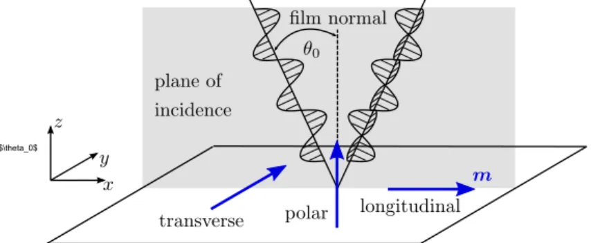
Figure 1.1.:

Coordinate system used in this work.

romagnetic film always lies within the x, y plane with a thickness d ≪ L, w . The angle between the magnetization and the z axis is θ and the angle of the in-plane component of M with respect to the x axis is defined as ϕ .

1.1. Micromagnetism

In general, magnetism is purely a quantum mechanical phenomenon. To describe, for example a metallic ferromagnet, (FM) such as Ni or Co one needs to treat a many-body problem taking into account the electronic structure of the respective crystal and addi- tionally the spin of the electrons. This can be done using e.g. density functional theory.

However, if one wants to describe the magnetization dynamics of a macroscopic sample it,

is impossible to use these methods due to the large number of atoms involved. It is there-

fore convenient to transfer the microscopic properties to a continuum theory describing

the time evolution of the sample’s magnetization under the influence of different torques

[Kob13; Coe10; Sto06; Ber09]. This continuum theory is called micromagnetic theory. It

describes the magnetization at every point in the ferromagnet as a vector function of space

and time, M ( r, t ). Using this formalism, analytic solutions can be derived for uniform

1. Magnetization Dynamics I: Energy Terms and Equation of Motion

and nonuniform, linear and nonlinear magnetization dynamics as e.g. spin waves in thin magnetic films [Ber09; Gur96]. The same formalism, however, can be discretized onto a grid to carry out micromagnetic simulations, which allows to study magnetization dynam- ics that cannot be described analytically due to the complex magnetic interactions in real ferromagnetic devices. The key advantage of micromagnetic theory is that the size of the grid in these simulations can be chosen much bigger than the lattice constant of the FM crystal treated. The procedure is therefore also called coarse-graining [Gri03] and has to be treated with caution in certain situations.

The key assumption of the theory in general is ∣ M ( r, t )∣ = M

at every point. The sat- uration magnetization M

=

is the sum over all microscopic magnetic moments µ in a given (cell) volume V . This is true if the temperature is much smaller than the Curie temperature such that the exchange dominates over all the other energies at the smallest scale treated [Ber09]. Due to this restriction it is always possible to normalize M ( r, t ) by dividing by M

and to use m ( r, t ) =

to describe a system with the unit vector of the magnetization m . In micromagnetic simulations, where the system is discretized into cells with dimensions dx, dy, dz , this constraint means that one cell always has a magnetic moment of µ

= M

V

or, differently spoken, M

= M

. The dimensions of the cells must then be chosen such that the magnetization direction varies only slightly between two neighboring cells, leading to cell sizes in the nm range, for short ranged problems such as e.g. domain walls, up to several µm, for long ranged problems as e.g. magnetostatic spin waves with wavelengths of tens of µm. In this work, micromagnetic simulations were carried out using the mumax

package which is documented in [Van14].

1.2. Energy Contributions

In a FM the spatial distribution of m ( r, t ) is given by the minimum of the free energy of the FM, E , that contains contributions from different origins. The total energy E =

∫

dV (∑ ε) is evaluated as an integral over the whole FM volume, where the integrand is a sum of the different local energy densities ε that will be discussed in the following. What makes ferromagnetism such a rich field, is the fact that the energies at play do have very different scales both in strength as well as in their interaction range. A good example for this is the domain structure in perpendicular magnetized, ultrathin Co layers which arises due to the counterplay of the strong but short-ranged exchange interaction and the weaker but long ranged dipolar interaction. A broken symmetry at interfaces in combination with spin orbit coupling in such a system can give rise to a second, antisymmetric exchange called Dzyaloshinskii-Moriya interaction, which will have additional impact on the domain pattern. Since micromagnetism is a continuum theory, all energies need to be derived in continuous form.

8

1.2. Energy Contributions

1.2.1. Exchange interaction

The fundamental energy contribution in a FM is the exchange interaction between elec- trons which enables ferromagnetic ordering. The origin of exchange is purely quantum mechanical and results from the coulomb interaction between electrons in combination with the Pauli exclusion principle. It is directly proportional to the overlap of the spatial wavefunctions of the respective electrons and therefore is a short ranged interaction [Sto06, chapter 6]. For electrons with spin S that are localized at lattice points i the exchange interaction can be expressed by the so-called Heisenberg Hamiltonian [Coe10]

H

= −2 ∑

i>j

J

S

⋅ S

(1.1)

where J

represents the exchange constant between electrons on site i and j . If only nearest neighbors are taken into account, J

can be simplified to a single exchange constant J for the whole lattice. In micromagnetics this Hamiltonian is expanded into a Taylor series [Chi10; Kit49; Kob13] and results in a continuous form such that the energy density reads [Ber09]

ε

= A ((∇m

)

+ (∇m

)

+ (∇m

)

) . (1.2) Here, V is the volume of the ferromagnet and A is the exchange stiffness constant which can, for a cubic lattice, be related to the exchange constant J by A =

[Kit49; Chi10].

Here n is the number of atoms in a unit cell, S is the eigenvalue of the spin operator and a is the lattice parameter. Values for A are 13 pJ/m for Py [Van14] and (10-16) pJ/m for ultra-thin Co [Mik15; Thi12].

1.2.2. Dzyaloshinskii-Moriya interaction

In systems with reduced symmetry and strong spin orbit coupling an additional, antisym- metric exchange interaction has been found in the 1960s by Dzyaloshinskii and Moriya [Dzy58; Mor60a; Mor60b] in crystals without inversion center. It has the general form

H

= − ∑

i>j

D

⋅ (S

× S

). (1.3)

Here, D

is the DM vector that is constructed from the symmetry of the crystal [Mor60a].

In contrast to the usual exchange interaction, the DMI tends to align spins perpendicular

to each other and thereby favors magnetic textures that exhibit large gradients in m(r, t)

such as domain walls [Thi12]. In the case of ultrathin magnetic multilayers the inversion

symmetry is broken at the interface which can lead to the emergence of a DMI even for

FMs that show no such interaction in the bulk state [Thi12; Cré98]. This form of DMI is

therefore called interfacial DMI (iDMI). For the case of a NM/FM/oxide layer structure

1. Magnetization Dynamics I: Energy Terms and Equation of Motion

the continuous form of the iDMI can be written as [Thi12]

ε

= D [ m

∇ m − ( m ⋅ ∇) m

] (1.4) Here, D is the iDMI constant. The strength of the iDMI in Pt/Co/Al

O

(MgO) multilay- ers has been measured extensively the last years resulting in values from D ⋅ d

∼0.3 pJ/m [Lee14b; Ben15] to 2 pJ/m [Kim15; Pai16; Bel15]. The exact value strongly depends on the interface [Kim17], which itself is strongly influenced by the growth conditions [Kim15].

1.2.3. Magnetostatic energy

The second class of energy densities is based on dipolar interactions between magnetic moments µ

. It should first be mentioned that the energy of a magnetic moment in an external field H

, the so-called Zeeman energy is given by

E

= − µ

µ ⋅ H

⇔ ε

= − µ

M

m ⋅ H

(1.5) where the local energy density for the continuous case is given on the right-hand side. In a FM the magnetization at each point is subject to the field generated by the dipolar fields of the magnetic moments of the whole volume of the FM. The dipolar energy of two magnetic moments can be written as [Chi10, chapter 1]

E

= − µ

µ

⋅ H

= − µ

4π∣r∣

(3( µ

⋅ ˆ r )( µ

⋅ r ˆ ) − µ

⋅ µ

) (1.6) where r is the vector connecting the two magnetic moments in space. The first equality of the equation shows that the energy can be written in the form of Eq. (1.5), e.g. the energy of two dipoles is given by the Zeemann energy of µ

in the field generated by µ

, here labeled H

. If the FM is pictured in discretized form the field H

acting on the moment µ

is the sum over the dipole fields generated by all remaining magnetic moments µ

H

= 1 4 π ∑

j

( µ

∣ r

− r

∣

− 3 ( µ

⋅ ( r

− r

))( r

− r

)

∣ r

− r

∣

) . (1.7) The field H

is often called stray field outside the FM and demagnetizing field inside the FM. This sum can be converted into a continuous integral form which reads [Her09]

H

( r ) = M

4 π ∫ dV

( r − r

)∇ m

∣ r − r

∣

+ M

∫ dS

( r − r

) m ⋅ n

∣ r − r

∣

(1.8) where the first integral is taken over the volume of the FM and the second integral over its surface and n is the surface normal unit vector. The above equation can be interpreted

1 note the different definition of magnetic moment in this book: M=µ0µ.

10

1.2. Energy Contributions as follows: there are two distinct sources of the demagnetizing field, one is ∇ m inside the bulk of the FM, which can therefore be identified as volume charge. On the boundary of the FM, m⋅ n gives the directional derivative of m perpendicular to the surface and hence acts like a surface charge. Both charges build up a demagnetizing field that points into the opposite direction of m inside the FM, hence the name demagnetizing field.

Another approach to obtain H

is based on Maxwell‘s equations in matter. First it should be noted that, without current flow, the magnetic flux is given by B = µ

( H

+ M ) with

∇ B = 0 and ∇× H = 0. It follows ∇ H

= −∇ M which is formally equal to the electrostatic equation ∇ E =

with the charge density ρ . By associating a vector potential such that H

= ∇ U

the Poisson equation ∆ H

= ∇ M has to be solved in order to find the demagnetizing field. It should be stressed that, in absence of other sufficiently strong fields, M is determined by H

, which again depends on the magnetization such that finding the equilibrium position is highly nontrivial. Both the magnetization and the demagnetizing field are in general non-homogeneous throughout the FM if the form of the FM is not highly symmetric. There are cases, however, where the integration of Eq. (1.8) can be carried out analytically. This is the case for ferromagnetic ellipsoids, in which both the magnetization and the demagnetizing field are homogeneous and are related via a linear equation:

H

( r ) = − M

N m. (1.9)

Here, N is the so-called demagnetization tensor which can be diagonalized if the coordinate system ( x, y, z ) is in accordance with the main axes of the ellipsoid which will be labeled a, b, c . Then, only N

, N

, N

are nonzero and N

∈ [0 , 1] while the trace is N

+ N

+ N

= 1.

The values for N

are calculated in [Osb45] for different limiting cases of ellipsoids. One example of a highly symmetric ellipsoid is a sphere, where the tensor elements are N

=

. In this thesis, thin films are treated, which can be approximated as infinitely flat oblate spheroids a ∼ b ≫ c for which only one element of the demagnetizing tensor is nonzero:

H

= − M

N

m

z, ˆ N

= 1 (1.10)

If a structure, for example a (infinitely long) stripe is patterned out of the film which has

dimensions L > w ≫ c , where usually L, w ∼ µm (with e.g.

> 10) and d ∼ nm, the demag-

netization field is not homogeneous across the width of the stripe. It is possible, however,

to define an average demagnetizing field over the whole volume of the FM such that, if the

magnetization is saturated e.g. by an external field, H

∶= − N

M

. Often

the approximation of an infinitely long elliptic cylinder is used, for which N

≈ 0, N

≈

and therefore N

≈ 1 −

; even though the geometry has the form of a rectangular prism

and not of an ellipsoid due to the ease of the form of N

. For rectangular prisms such

1. Magnetization Dynamics I: Energy Terms and Equation of Motion

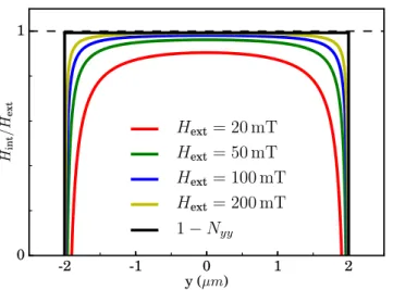
demagnetizing factors are calculated in [Aha98] and compared to the elliptical case. Such a treatment allows estimating the impact of the demagnetizing field on e.g. the ferromag- netic resonance frequency of a stripe like device in saturated case but fails to predict the effects of the inhomogeneous demagnetization fields, which is most prominent in the case of low externally applied fields.

Finally, the energy density due to the demagnetizing field is given by:

ε

= − µ

M

2 m ⋅ H

(1.11)

where the factor of two accounts for double counting. For the special case of a thin film/an infinitely long stripe this contribution can be written as

ε

= µ

M

2 m

., ε

= µ

M

2 ( N

m

+ N

m

) . (1.12) It is directly clear from these equations that, in order to minimize the energy, the mag- netization must lie in the film plane. To pull the magnetization out of plane, a large energy has to be provided by other sources. The effect of the demagnetizing field is there- fore called shape anisotropy. Depending on the geometry of the FM, preferred directions for the magnetization exist resulting in a low demagnetizing energy which, are called easy axes/planes and directions with high demagnetizing energy, which are called hard axes/planes. For a thin film, regarding only the shape anisotropy, the film plane is the easy plane and the normal of the plane is the hard axis. Assuming a saturation magneti- zation of µ

M

= 1 T/1.8 T for Py/Co this gives an energy difference of 398/1289 kJ/m

between an inplane (ip) and out-of-plane (oop) magnetized state.

1.2.4. Crystalline anisotropy

In all of the 3d transition metals Fe, Co and Ni a second type of anisotropy exists, that depends on the symmetry of the crystal lattice and is therefore called magneto-crystalline anisotropy. In these metals the 3d orbitals are partially filled and therefore determine the electronic and magnetic ground state. Due to the crystal structure of these metals, the orbital moment of the 3d states is quenched and the magnetism is carried mainly by the spin moment. The quenching is a result of the strong interaction of the 3d orbits with the crystal field created by the neighboring atoms which reduces the orbital moment to zero.

However, via spin orbit coupling, a small part of the orbital moment is recreated. This orbital moment is now linked firmly to the lattice and the spin orbit coupling transfers this dependence on the spin moment. [Sto06; Coe10; Blu01]. This creates an energy density that depends on the symmetry of the crystal and is usually expressed in the coordinate system of the respective crystal by defining direction cosines (projection of m onto a given direction) α

= m ⋅ e ˆ

. Here, ˆ e

is a crystal axis unit vector. For a cubic lattice, the crystal

12

1.2. Energy Contributions axes coincide with an appropriate Cartesian coordinate system such that the unit vectors are x, y, z and therefore α

= m

, i = x, y, z . The lowest order energy density has fourfold symmetry and reads [Coe10; Wol04; Mei14]:

ε

= K

( α

α

+ α

α

+ α

α

) = K

2 (1 − α

− α

− α

) . (1.13) In this work two different FM systems are studied. The first FM used is Permalloy (Py) which is a Ni

Fe

alloy designed such that the magneto-crystalline anisotropies of Fe and Ni (both having a cubic lattice) cancel each other and the result is a soft magnetic material with no significant crystalline anisotropy [Yin06].

The other system is a Pt/Co(0.5 nm)/Al

O

multilayer that deserves special attention.

The layer structure is chosen such that the FM is magnetized perpendicular to the film plane, i.e. a very high anisotropy is present that overcomes the demagnetizing energy.

Bulk Co has a hexagonal lattice structure with one preferred axis, the c-axis. Therefore the corresponding bulk anisotropy is uniaxial instead of cubic, with a very weak six-fold anisotropy. However, when thin Co layers are grown onto a Pt(111) layer, the Co layer adopts to the Pt fcc structure and therefore has cubic symmetry [Wel94; Nak98; Ole00;

Wel01]. The volume anisotropy of fcc Co in bulk-like samples (several 1-10 nm thick) has been measured to be in the order of K

= 70 kJ/m

[Suz94; Fas95], which is two orders of magnitude smaller than the shape anisotropy. Additionally, the fourfold anisotropy constant vanishes for sub-nm thickness [Fas95] and no sizable in-plane anisotropy is present in Pt/Co multilayers [Wel94] such that for a 0.5 nm thick Co film on Pt(111) the magneto- crystalline anisotropy from the bulk can be neglected.

1.2.5. Interface anisotropy

The physical origin for the perpendicular easy axis of the Pt/Co(0.5 nm)/Al

O

is the inter- action of Co with Pt and Al

O

at the respective interface. The perpendicular anisotropy induced by this effect is therefore called interfacial anisotropy. A detailed explanation of the physics of this anisotropy term, based on the model of Bruno [Bru89], can be found in [Sto06, chapt. 7.9].

Bruno has shown theoretically that for more than half-filled d-shells the magnetic anisotropy energy is directly linked to the anisotropy of the orbital moment ε

∝ −( m

− m

) cos

₍ θ ) [Bru89; Wel94; Wel95]. This theoretical prediction has been confirmed by measurements of both the anisotropy constant and the orbital momentum in Pt/Co, Pd/Co and Ni/Co multilayers [Wel94] as well as on a Au/Co-wedge/Au sandwich [Wel95].

A

dependence is found indicating that indeed the interface plays a dominant role.

To understand the origin of the PMA in Pt/Co(0.5 nm)/Al

O

it must be known how the

orbital moments of the interfacial Co atoms are deformed to lead to an imbalance of ip and

1. Magnetization Dynamics I: Energy Terms and Equation of Motion

oop orbital moment. It appears that both interfaces lead to a deformation of the Co 3d orbitals in a very similar manner. At the Pt(111)/Co interface, the Co 3d band hybridizes with the Pt 5d band which can be viewed as an effective uniaxial crystal field acting on the Co atoms [Nak98; Man08a]. This effect thus acts at the interface only and leads to a

dependence of the anisotropy energy. This prediction was confirmed by measurements of the magnetic moment of single Co adatoms and clusters on a Pt(111) substrate [Gam03].

At the Co/Al

O

interface the PMA stems from covalent Co-O bonds between the oxygen 2p orbitals and the Co 3d orbitals [Ole00; Mon02; Man08a]. In an experiment similar to the abovementioned study the orbital moment of Co adatoms on the oxygen site of a MgO single crystal have been studied and a huge PMA has been found which was again attributed to an uniaxial ligand field at the O site as a result of the covalent bond [Rau14].

The energy density from one interface can therefore be written as [Kim17]

ε

= − K

d

cos

( θ ) = − K

d

m

. (1.14)

Here, the unit of K

is [J/m

]. Since there are two different interfaces, the respective terms have to be added up. The thickness dependence allows to separate the interface contribution from bulk anisotropies and if either interface can be changed independently, the contributions of both interfaces can be disentangled, see e.g. [Kim17]. In the present work an effective oop anisotropy constant resulting from both interfaces is used as input for calculations and micromagnetic simulations which is given by

ε

= − K

m

(1.15)

with the effective oop anisotropy constant K

=

. As the thickness of the Co layer in this work is ∼ 0.5 nm, a large enough value for K

is reached to overcome the demagnetization energy.

Pure Py and NM/Py films grown onto GaAs substrate and capped with an oxide layer in most cases show an oop uniaxial anisotropy of similar origin. However, due to the fact that the Py thickness is in the nm range, the corresponding K

is much smaller than the demagnetizing energy.

In addition, it is known that Fe, Ni and Fe-Ni alloys grown on GaAs exhibit an additional in-plane uniaxial anisotropy, caused by the GaAs/FM interface [Yin06; Was05]. Such an ip uniaxial anisotropy can be expressed as [Wol04; Was05]:

ε

= − K

( n ˆ ⋅ m )

(1.16) with the ip unit vector ˆ n is pointing along the direction of minimal energy. This anisotropy is very small in the samples measured in this work, the order of magnitude is 400/80/1

14

1.3. Landau-Lifshitz-Gilbert Equation for shape/oop/ip anisotropy energy density even for the thinnest (4 nm) measured Py films.

However, in the evaluation of ferromagnetic resonance data, even a small ip anisotropy can influence the fitting results for the other parameters and should be included in the analysis.

1.3. Landau-Lifshitz-Gilbert Equation

The knowledge of the energy contributions allows to find the equilibrium position of the magnetization by minimizing the free energy under the restraint ∣M∣ = M

. However, if the magnetization is out of equilibrium, an appropriate equation of motion is needed to describe the dynamics of the system. This requirement is met by the Landau-Lifshitz- Gilbert equation (LLG) that describes the time evolution of a magnetic moment in an effective field H

[Ber09]:

∂m

∂t = − γ m × ( µ

H

) + α m × ∂m

∂t = T

+ T

. (1.17) Here γ is the gyromagnetic ratio and α is the Gilbert damping parameter. Since the change in magnetization is always perpendicular to m , the LLG is a torque equation such that any terms on the right-hand side are labeled T

.

The first term on the right-hand side is called precessional torque, since a misalignement of M and the effective field H

leads to a precession of the magnetization around H

. The precession frequency is determined by the gyromagnetic ratio γ . For a free electron, γ = 176 × 10

and therefore the precession frequency f =

= −

µ

H

lies in the GHz frequency range for an effective field µ

H

∼ 100 mT, a typical value for the experiments in this thesis

.

The second torque, proposed by Gilbert 1955 [Gil55]

introduces a viscous type damping where α determines the strength of the damping. In most FMs used for dynamic exper- iments α is small, ∼ 0 . 008 in the Py films studied in this work but it can also be rather large, on the order of 0 . 5 for the ultra-thin Co grown on a Pt underlayer as will be detailed later.

The effective field introduced in the LLG equation comprises all different energy terms

2 letθ be the angle betweenM and H,H∣∣z, andϕthe angle describing the movement of M in thex, y plane, neglect the damping term. Then ^∂M_∂t =Mcos(θ)^∂ϕ

∂t =µ0γM Hcos(θ) ⇒ ^∂ϕ

∂t =ω=γµ0Heff. This simple calculation holds only if the effective field does not depend onM.

3 [Sas09] gives a review about the form of the damping term and about this “special” reference which is always cited but cannot be found.

1. Magnetization Dynamics I: Energy Terms and Equation of Motion

introduced before. Field and energy are connected via

H

= − 1

µ

M

δε

δm (1.18)

where the index i stands for the respective energy term [Ber09]. Altogether, the effective field of a thin film is therefore given by [Ber09; Van14]

H

= H

+ H

+ H

+ H

+ H

= 2A

µ

M

∆m + 2D

µ

M

( ∂m

∂x , ∂m

∂y , − ∂m

∂x − ∂m

∂y ) − M

m

+ 2 K

µ

M

m

+ H

. (1.19) From the LLG, the equilibrium of m is simply given by the condition m

× H

= 0 and therefore m

∥ H

.

In the last years it has been found that the injection of a charge current into NM/FM heterostructures influences the magnetization dynamics of the FM layer, i.e. additional torques on the magnetization are observed experimentally. These torques are called “spin orbit torques” (SOT) due to their physical origin, the spin orbit coupling [Gar13]. These additional torques must be included in the LLG equation. Due to the fundamental restric- tion of conservation of ∣ M ∣ any given torque acting on m can be decomposed into two orthogonal torques of the form

T

= −γ τ

m × σ

T

= γ τ

m × ( m × σ

) (1.20)

where σ

is a unit vector [Ber09]. Here the torque of T

corresponds to the addition of another field H ∥ σ to the effective field and induces a precession of m around σ

if no other torque is present. Hence such a torque will be named field-like torque in the following. It can just be added to the effective field torque.

The form of T

is of fundamental difference since this torque directly moves the magne- tization to the direction of σ . The vector component of σ that is parallel/antiparallel to H

will counteract/enhance the damping torque T

, hence it is called damping-like torque. In the general case where σ ∦ H

the equilibrium position must be calculated from T

+ T

= 0 and is therefore no longer given by M

∥ H

.

4the variation in this equation reduces to a simple derivative for all fields created by non-space dependent energy contributions like the anisotropy fields etc. For the exchange energy, the calculation is more difficult and results in the expression given below [Ber09; Van14]. The derivative with respect to m is, strictly speaking, a directional derivative on the surface of the sphere with radius Ms due to the conservation of the magnetization vector’s length. This should be kept in mind when doing calculations in Cartesian coordinates, especially when plotting anisotropy fields etc. However, the effective field can be calculated by applying the full gradient in all 3 Cartesian dimensions, as done e.g. in mumax³ [Van14] and still be used in the LLG equation because the cross product ignores the components that are not perpendicular tom. The author wants to thank Johannes Stigloher and Martin Buchner for a fruitful discussion of this (sometimes) important detail.

16

1.3. Landau-Lifshitz-Gilbert Equation

Including the additional SOTs, the generalized LLG reads

∂m

∂t = − γ m × ( µ

H

+ τ

σ

) + αm × ∂m

∂t + γτ

m × ( m × σ

) . (1.21) To solve the LLG numerically, it is common to transform it into its explicit form

which can be handled by standard ODE solvers and reads:

∂m

∂t = γ

1 + α

{ − m × ( µ

H

+ τ

σ

) + τ

m × ( m × σ

)

− α [ m × ( m × ( µ

H

+ τ

σ

)) − τ

m × σ

]} .

(1.22)

This equation is also basis of the micromagnetic simulations package mumax

used in this work, see [Van14].

5without the additional torques, the transformation converts the LLG into the mathematically equivalent Landau-Lifshitz equation of motion, see [Ber09, p. 27f].

2. Spin Orbit Torques in Metallic Multilayers

The key for an efficient manipulation of NM/FM/oxide elements via electrical currents lies in the so-called spin orbit torques that are created by spin currents and spin accumulations either at the NM/FM or FM/oxide interface and/or in the bulk of the NM. The name spin orbit torque already implies that the origin of theses effects lies in the spin orbit coupling. Measurements of current induced torques in FM/NM/Oxide multilayers have shown that both field-like and damping-like torques are present in general, however, the relative strength and sign differ from multilayer to multilayer, depending on the single layer properties as well as on the interfaces of the NM. It is therefore quite puzzling to find out about the microscopic origins of the torques and to make quantitative predictions in order to engineer the layer structures for a given application.

There are two distinct scenarios that lead to a torque on the magnetization: If a spin accumulation in the FM itself is created by some mechanism and if this spin accumulation is not collinear with the magnetization, the spin accumulation will start to precess around the local magnetization due to exchange coupling. Vice versa, the magnetization precesses around the spin accumulation giving rise to a field-like torque. In the second case, a spin current enters a FM at an interface and is absorbed, thereby transporting angular momentum to the FM. In this case the torque on the magnetization has a damping-like form.

There are two distinct physical effects that have evolved as explanation for the appearance of the experimentally observed torques which will be discussed below, namely the spin Hall effect (SHE) and the Rashba-Edelstein (REE) effect. Thus, in the following the concept of spin accumulation and spin current will be introduced. Afterwards, both SHE and REE will be introduced and it will be shown how these effects can create a torque on the magnetization.

2.1. Spin and Charge Currents

In this section the concept of spin currents and spin accumulations shall be introduced.

Phenomenologically, these quantities can be understood well in the context of the drift

diffusion formalism. Therefore, in the following the drift diffusion equations for both

charge and spin transport will be introduced for NMs first and then be generalized for FMs,

following the respective sections in [Fab07; Obs15] in accordance with [Dya12; Han13a].

2. Spin Orbit Torques in Metallic Multilayers

2.1.1. Drift diffusion equation for charge

In metals, electric transport can be described by a drift diffusion model if the dimensions of the device are much bigger than the mean free path and the system is only distorted little from equilibrium. In this case, the drift diffusion equation for the electron charge density is given by [Fab07]

−∣ e ∣ ∂n

∂t + ∇ j

= 0 j

= σE

+ ∣ e ∣ D ∂n

∂x

= σ (∇ µ )

.

(2.1)

Here, n is the electron particle density, j

= −∣e∣j

is the charge flow in direction i, where j

is the particle current, σ =

and D =

are the electrical conductivity and the diffusion coefficient where τ is the momentum relaxation time, m the electron (effective) mass and v

the Fermi velocity. The first line is a continuity equation for the charge and the second line defines the charge current. The charge density at a given point in space can change only if there is a divergence in the charge current at this point. It is convenient to define an electrical effective potential µ such that the current can be written as j

= σ ∇ µ . The drift diffusion equation is solved for µ and the current can be calculated subsequently.

2.1.2. Drift diffusion equation for spin

Similar equations describe the spin drift and diffusion, however, due to the nature of spin transport two important differences occur. The first difference between charge and spin drift and diffusion is the fact that there is no conservation for the spin and an additional relaxation term is added to the continuity equation for the spin. The second difference is that the spin current has two degrees of freedom. A spin current is therefore described by a second rank tensor j

with entries j

where the first index denotes the spatial coordinate and the second index denotes the spin polarization direction. Consider first a NM where a spin (particle) accumulation can be defined as s

= n

− n

where n

is the number of electrons with spin pointing in ± x

-direction. The spin momentum accumulation is then

̵h

2

s . In a NM all parameters, e.g. like σ , are the same for electrons regardless of their spin direction and the drift diffusion equation can be written as [Fab07]

0 = ̵ h 2 [ ∂s

∂t + s

τ

] + ∂j

∂x

j

= ̵ h

2 [− µ

E

s

− D ∂s

∂x

] .

(2.2)

In this equation τ

is the (isotropic) spin relaxation time. A characteristic length that coincides with this time is the so-called spin diffusion length λ

= √

Dτ

. The origin of

20

2.1. Spin and Charge Currents spin relaxation in metals is usually attributed to the Elliot-Yafet relaxation mechanism [Ell54; Yaf63]. The basic idea of this model is that every momentum scattering event has a certain probability to also switch the spin, which implies τ

= P τ with the probability factor P which must be smaller than one. The constant µ

in the definition of the spin current denotes the mobility and should not be confused with the quasichemical potential µ.

The equations can also be expressed in terms of a quasichemical potential for the spin µ

which is, in contrast to the charge current case, a vector that points in the direction of the spin polarization. For the steady state

= 0 the equations reduce to [Ami16b; Fab07]:

∇

µ

= µ

λ

j

= ̵ h

2∣ e ∣ σ ∂µ

∂x

(2.3)

It should be noted that the spin quasichemical potential and the spin particle accumulation are related by s = g (

)∣ e ∣ µ

, where g denotes the density of states at the Fermi level. From the definition of the spin current it can be seen that there are two different cases of spin transport: if there is a spin accumulation and an electric field, the electrons will drift due to this field and in addition carry a net spin current. This situation is referred to as a spin polarized current. On the other hand, a non-homogeneous spin accumulation will lead to a diffusion of spin density, i.e. a spin current, without any charge transport. This is what will be called a (pure) spin current in this thesis.

2.1.3. Drift diffusion in ferromagnets

In an itinerant FM, transport is usually split up into two channels for majority and minority electrons. Let ↑ / ↓ denote the majority/minority electrons

. The total charge current is given by the sum of the currents carried by both channels, j

= j

+ j

. The conductivity is different for both spin populations, and is defined as σ

. Then σ = σ

+ σ

is the overall conductivity, σ

= σ

− σ

is defined as the spin spin conductivity and P

=

as the conductivity spin polarization. In a FM, the quantization axis is naturally defined by the magnetization and usually the coordinate system is chosen such that ↑ , ↓∥ m ∥ z ˆ . If the spin polarization in the FM is allowed to have components in any direction, the charge

1It should be kept in mind that the majority electrons carry spin which is antiparallel to the magnetization unit vectorm.

2.2. Spin Hall Effect

and spin current in the FM are [Han13a]:

j

= σ ∂

∂x

µ − P

σ ∂

∂x

( m ⋅ µ

) j

= ̵ h

2∣ e ∣ [P

σm

∂

∂x

µ − σ ∂

∂x

µ

] .

(2.4)

For P

= 0 these equations reduce to the NM case. In an itinerant FM charge transport is usually accompanied by spin currents due to the fact that the total current is spin polarized.

The same holds the other way; if there is a spin current due to a non-homogeneous spin density, there will be an additional charge current. There are, however, physical effects that couple even pure spin and charge currents in a NM as well in a FM. These effects will be introduced in the next section.

It should be noted that the drift diffusion equations in the FM need to be extended in order to take into account the (damped) precession of the local, nonequilibrium spin density around m as will be described in detail in sect. I.2.3 [Han13a]:

h ̵ 2 [ ∂s

∂t + s

τ

+ 1

τ

s × m + 1

τ

m × ( s × m )] + ∂j

∂x

= 0 . (2.5)

In this equation, the term

s × m describes the precession of a spin accumulation around the local magnetization due to exchange coupling and the term

dp

m × ( s × m ) describes the damping of this precession, i.e. the absorption of the transverse component of s with respect to m. This damping process is very fast in the metallic ferromagnets treated in this work. Therefore any noncollinear spin accumulation that is the result of a spin current entering the FM at an interface, is absorbed in the FM within a few lattice constants [Sti02]. It is therefore convenient to drop the two terms in the drift diffusion equation and shift the absorption of a spin current into the boundary conditions instead [Han13a].

However, if there is a source of spin accumulation within the bulk of the FM, the precession has to be taken into account explicitly as shown in sect. I.2.3.

2.2. Spin Hall Effect

The spin Hall effect (SHE) describes the phenomenon of the conversion of a charge current into a transverse pure spin current. The SHE has been proposed in 1971 by Dyakonov and Perel [Dya71a; Dya71b] but was brought to the attention of the spintronic community only by Hirsch in 1999 [Hir99] and subsequently by Zhang (2000) [Zha00]. The first experimental observation has then been realized in 2004 [Kat04; Wun05] in semiconductors.

Since then the SHE has been explored as an efficient way to manipulate and even switch the magnetization in NM/FM bilayers by charge current injection [Mir11; Liu12b; Liu12a].

A comprehensive review of the spin Hall effect has recently been published by Sinova et

22

al. [Sin15] and is followed throughout this section.

Under the influence of spin orbit interaction, spin and charge currents become coupled in such a way that from a charge current a transverse spin current is created and vice versa.

In the drift diffusion formalism, the spin orbit interaction connects the equations for spin and charge currents via a constant θ

that is called the spin Hall angle 0 < θ

< 1 [Dya12]:

j

= j

+ 2∣ e ∣

h ̵ θ

j

j

= j

− h ̵

2∣ e ∣ θ

j

.

(2.6)

Here

is the Levi-Civita symbol, and j

/j

are the charge/spin currents without spin orbit coupling. The polarization of the spin current is always perpendicular to both charge current and spin current flow direction. For a positive θ

the polarization unit vector σ = n × ˆ j

with the spin current flow direction n [Dec12]. The modified expressions for charge and spin current then read explicitly [Sin15; Dya07; Obs15]:

j

= σE

+ ∣ e ∣ D ∂n

∂x

− ∣ e ∣ θ

[ µ

E

s

+ D ∂s

∂x

] (2.7)

j

= h ̵

2 {−µ

E

s

− D ∂s

∂x

− θ

∣ e ∣

[σE

+ ∣e∣D ∂n

∂x

]} . (2.8)

The third term in Eq. (2.7) corresponds to the anomalous Hall effect (AHE) and describes the creation of a transverse charge current if a spin polarized current flows in a material.

This effect is known in the context of transport in FMs. The fourth term is the inverse spin Hall effect (ISHE), here a transverse charge current is created by a pure spin current.

The distinction between these two terms has only arisen historically because the AHE was experimentally found already in 1881 by E. H. Hall (in FM), in contrast to the ISHE which was discovered only recently. The reason for this discrepancy is that in a FM a spin-polarized current can be created easily by applying a dc current. The AHE can be measured easily by picking up the transverse voltage. By contrast to this, the creation of a pure spin current and a subsequent measurement of the resulting spin accumulation has become possible only recently. For the reciprocal effect, such a distinction is not existent:

the third and fourth term in Eq. (2.8) together are called spin Hall effect and describe the creation of a pure spin current from a charge current.

The physical origin of the conversion is the same in all cases and has provided a puzzle

for theoretical physicists for a long time. The theory of AHE has evolved since the first

discovery over 100 years ago finally providing a framework for the understanding of the

AHE and the SHE. A detailed description of the AHE and its history can be found in

[Nag10]. There are three semiclassical origins of the SHE and AHE, related to different

microscopic origins: i) skew scattering, ii) side jump and iii) intrinsic SHE. The first two of