K. Burmeister1 , J. F. Lübbecke1,2 , P. Brandt1,2 , and O. Duteil1
1GEOMAR Helmholtz Centre for Ocean Research Kiel, Kiel, Germany,2Christian-Albrechts-Universität zu Kiel, Faculty of Mathematics and Natural Sciences, Kiel, Germany
Abstract
The North Equatorial Undercurrent (NEUC) has been suggested to act as an important oxygen supply route toward the oxygen minimum zone in the eastern tropical North Atlantic.Observational estimates of the mean NEUC strength are uncertain due to the presence of elevated mesoscale activities, and models have difficulties in simulating a realistic NEUC. Here we investigate the interannual variability of the NEUC and its impact onto oxygen based on the output of a high-resolution Ocean General Circulation Model (OGCM) and contrast the results with an unique data set of 21 ship sections along 23◦W and a conceptual model. We find that the interannual variability of the NEUC in the OGCM is related to the Atlantic meridional mode with a stronger and more northward NEUC during negative Atlantic meridional mode phases. Discrepancies between the OGCM and observations suggest a different role of the NEUC in setting the regional oxygen distribution. In the model a stronger NEUC is associated with a weaker oxygen supply toward the east. We attribute this to a too strong recirculation between the NEUC and the northern branch of the South Equatorial Current in the OGCM. Idealized experiments with the conceptual model support the idea that the impact of NEUC variability on oxygen depends on the source water pathway. A strengthening of the NEUC supplied out of the western boundary acts to increase oxygen levels within the NEUC. A strengthening of the recirculations between NEUC and the northern branch of the South Equatorial Current results in a reduction of oxygen levels within the NEUC.
Plain Language Summary
In the eastern tropical North Atlantic a zone of low-oxygen waters exists between 100 and 700 m due to high oxygen consumption and a weak exchange of water masses.Long-term oxygen changes in this zone have been reported with potential impacts on, for example, ecosystems including fish populations. The water masses in that region are exchanged among others via weak eastward and westward currents. The mean eastward-flowing North Equatorial Undercurrent (NEUC) transports oxygen-rich waters from the western basin into the eastern low-oxygen zone, suggesting that a stronger NEUC supplies more oxygen-rich water toward the eastern basin. In this study we investigate the year-to-year variability of the NEUC and its impact on oxygen. For our analysis, we are using ship observations and model simulations. We find some discrepancies between them that we attribute to a too strong recirculation between the NEUC and the westward-flowing current just south of it in the model. This recirculation impacts the variability of the eastward oxygen supply, as the westward current is transporting low-oxygen waters. In the model, a higher recirculation between the currents results in a stronger NEUC transporting lower-oxygen waters, a mechanism for oxygen variability that could not be conjectured from observations so far.
1. Introduction
The oxygen concentration in the oceans is controlled by the interaction of physical and biogeochemical pro- cesses. Oxygen is supplied to the ocean by photosynthesis or air-sea gas exchange, and it is transported into the ocean interior by advection and mixing (e.g., Brandt et al., 2015; Karstensen et al., 2008; Stramma et al., 2008). Oxygen is consumed by respiration, for example, by remineralization of sinking particles (Matear
& Hirst, 2003). Locally, advection and mixing can also act to decrease oxygen levels, depending on the background oxygen field (Brandt et al., 2010; Hahn et al., 2014).
The tropical Atlantic is characterized by a complex system of zonal currents that can transport oxygen-rich waters from the western boundary eastward toward the Eastern Tropical North Atlantic (ETNA) Oxygen
Key Points:
• Interannual variability of North Equatorial Undercurrent in an ocean general circulation model is linked to Atlantic meridional mode
• Oxygen supply by the North Equatorial Undercurrent toward the eastern tropical North Atlantic depends on the pathway of its source waters
• Different supply routes might explain discrepancies between simulated and observed oxygen supply by the North Equatorial Undercurrent
Supporting Information:
• Supporting Information S1
Correspondence to:
K. Burmeister, kburmeister@geomar.de
Citation:
Burmeister K., Lübbecke, J. F., Brandt, P., & Duteil, O. (2019).
Interannual variability of the Atlantic North Equatorial Undercurrent and its impact on oxygen.Journal of Geophys- ical Research: Oceans,124, 2348–2373.
https://doi.org/10.1029/2018JC014760
Received 12 NOV 2018 Accepted 10 MAR 2019
Accepted article online 14 MAR 2019 Published online 3 APR 2019
©2019. American Geophysical Union.
All Rights Reserved.
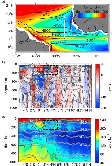
Figure 1.(a) Oxygen concentration in 𝜇mol∕kg (shaded colors) in the tropical Atlantic averaged between 100 and 200 m depth (depth range of North Equatorial Undercurrent [NEUC] core) obtained from MIMOC (Schmidtko et al., 2017). Superimposed are surface and thermocline (about upper 300 m) currents (black solid arrows; adapted from Hahn et al., 2017): the North Equatorial Current (NEC), Cape Verde Current (CVC), North Equatorial Countercurrent (NECC), northern branch of the NECC (nNECC), NEUC, northern branch of the South Equatorial Current (nSEC) and central branch of the South Equatorial Current (cSEC), Equatorial Undercurrent (EUC), South Equatorial
Undercurrent (SEUC), and Guinea Current (GC). The white bar denotes the 23◦W section between 0◦and 14◦N. The white dashed rectangle marks the model domain of the conceptual model. (b) Zonal velocity and (c) oxygen
observations along 23◦W obtained during Meteor cruise M145 from February to March 2018. The black dashed rectangles mark the region of a potential recirculation between the nSEC and NEUC.
Minimum Zone (OMZ) or oxygen-poor waters westward (Figure 1). Consequently, the zonal advection of oxygen-rich water masses from the western boundary by eastward-flowing ocean currents has been identi- fied as an important ventilation process for the ETNA OMZ, especially in the upper 130 to 300 m (Brandt et al., 2015; Hahn et al., 2014, 2017). The most important currents are the main wind-driven ones such as the Equatorial Undercurrent (EUC), the North Equatorial Undercurrent (NEUC), and the northern branch of the North Equatorial Countercurrent (nNECC; e.g., Bourlès et al., 2002; Peña-Izquierdo et al., 2015; Schott et al., 2004). Below the wind-driven ocean circulation, the flow field in the ETNA OMZ is characterized by eddy-driven, weak latitudinal alternating zonal jets (Ascani et al., 2010; Brandt et al., 2010; Maximenko et al., 2005; Ollitrault & Colin de Verdière, 2014; Qiu et al., 2013).
Oxygen levels in the ETNA OMZ are declining in accordance with global deoxygenation (Schmidtko et al., 2017; Stramma et al., 2008). Superimposed on this multidecadal trend are interannual to decadal variations.
The identification of the mechanisms of long-term oxygen changes is challenging because of large uncer- tainties in the observed oxygen budget terms (Hahn et al., 2017; Oschlies et al., 2018). Furthermore, large biases in the oxygen distribution in ocean models hamper the analysis of OMZ variability (e.g. Cabré et al., 2015; Dietze & Loeptien, 2013; Duteil et al., 2014; Oschlies et al., 2018, 2017; Stramma et al., 2012). One reason for an insufficient representation of eastern tropical OMZs in models is that state-of-the-art general circulation models have problems to realistically simulate the equatorial and off-equatorial zonal subsurface currents (Duteil et al., 2014).
Among the off-equatorial eastward subsurface current bands, the NEUC is associated with the highest oxy- gen levels in the eastern Tropical Atlantic basin (Figure 1). The NEUC is centered at 5◦N (Figures 1a and 1b) and is located at depth where zonal advection plays an important role in ventilating the ETNA OMZ (Hahn et al., 2014). The western boundary regime is ventilated by oxygen-rich water masses supplied by the North Brazil Current (NBC). The EUC, NEUC, and nNECC feed from the retroflection of the NBC (Bourlès et al., 1999; Hüttl-Kabus & Böning, 2008; Rosell-Fieschi et al., 2015; Stramma et al., 2005). The NEUC thus can supply oxygen-rich water masses from the western boundary toward the ETNA OMZ (Brandt et al., 2010;
Stramma et al., 2008). Although its mean velocity is comparable to that of the nNECC, its associated oxygen maxima along 23◦W has been observed to be several𝜇mol/kg higher (Figures 1b and 1c).
The underlying dynamics of the NEUC are still not fully understood. Several model studies show that the NEUC is mainly in geostrophic balance but they do not agree on its driving mechanism. Marin et al. (2000) studied the Pacific counterparts of the NEUC, the so called Tsuchiya jets or Subsurface Countercurrents, and compared their dynamics with the atmospheric zonal jets of the Hadley cell at around 30◦N. They suggest that the tropical cells are the oceanic dynamical equivalent to the Hadley cells, where the conservation of angular momentum plays a key role in explaining the zonal jets. Jochum and Malanotte-Rizzoli (2004) investigated the dynamics of the SEUC, the southern counterpart of the NEUC in the Atlantic. Their model results show that the Eliassen-Palm flux associated with the propagation of tropical instability waves (TIWs) can be one possible driver of such zonal currents. Other model studies in the Pacific suggest that the oceanic jets are pulled by the upwelling within domes in the eastern basin or by the eastern boundary upwelling (Furue et al., 2007, 2009; McCreary et al., 2002).
The NEUC is a weak and highly variable current. Its observed core velocity varies from below 0.1 m/s (Brandt et al., 2006) to over 0.3 m/s (Urbano et al., 2008). In ship sections the NEUC is likely to be biased by the high mesoscale activity present in the tropical Atlantic (e.g., Goes et al., 2013; Weisberg & Weingartner, 1988).
Furthermore, estimates of NEUC transport are difficult because a clear separation of the current cores of the NEUC, and North Equatorial Countercurrent (NECC) above is not possible (Figure 2a). Observational estimates range from 2.7 to 6.9 Sv in meridional ship sections taken between 38◦W and 35◦W (Bourlès et al., 1999, 2002; Schott et al., 2003, 1995; Urbano et al., 2008). Another problem is that some transport estimates from observations only cover part of the NEUC, as, for example, Brandt et al. (2006) calculated zonal current transports from a mean ship section along 26◦W. They found a transport of only 0.8 Sv for the eastward flow in the region of the NEUC along 26◦W but only covered the flow south of 5◦N.
Goes et al. (2013) used a synthetic method to estimate the NEUC transport between 30◦W and 23◦W. They combined expendable bathythermograph temperature with altimetric sea level anomalies to derive NEUC location, velocity, and transport. In the potential density layers of 24.5–26.8 kg/m3they found a NEUC trans-
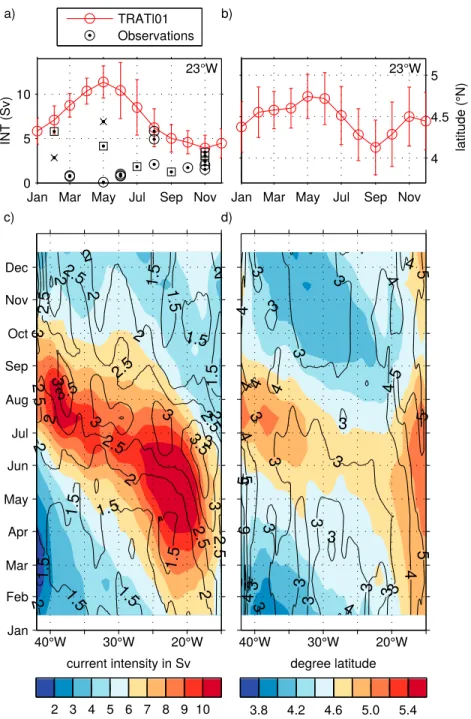
Figure 2.(a and b) Zonal velocity and (c and d) oxygen concentrations along 23◦W from (a and c) observations and (b and d) the output of TRATL01. The observed velocity field (a) is an averaged of 21 ship sections along 23◦W from 2002 to 2018, and the observed oxygen field (c) is an average of 11 ship section along 23◦W from 2006 to 2018. The TRATL01 output (b and d) is an averaged of the last 14 years of the model run (1994–2007) along 23◦W. (a and b) Eastward velocities are positive (red), and westward are negative (blue). Gray contours mark neutral density surfaces (kg/m3). Currents (in a) are the Equatorial Undercurrent (EUC), the northern branch of the South Equatorial Current (nSEC), the North Equatorial Countercurrent (NECC) and its northern branch (nNECC), the North Equatorial Undercurrent (NEUC), and the North Intermediate Countercurrent (NICC).
port varying from 2.3 Sv during August to October to up to 5.5 Sv during May and June. The core position of the NEUC in the synthesis product varies between 4.5◦N and 5.5◦N and exhibits a semiannual cycle with minima in April and September and maxima in August and December. Their estimated NEUC core veloc- ities were highest in June (above 0.3 m/s) and lowest during boreal fall (below 0.2 m/s). In a model study, Hüttl-Kabus and Böning (2008) found a clear seasonal cycle of the NEUC at 35◦W and 23◦W with maxi- mum NEUC transports (4.5–7.0 Sv) between May and June, and minimum transports (1.2–4.2 Sv) between September and October. They found a westward propagation of the seasonal cycle consistent with annual Rossby wave patterns (Böning & Kröger, 2005; Brandt & Eden, 2005; Thierry et al., 2004).
In ship sections the NEUC shows no clear seasonal cycle. Four transport estimates exist between 35◦W and 38◦W during boreal spring from 1993 to 1996 (Bourlès et al., 1999; Schott et al., 1995). In the same depth range as in Goes et al. (2013) and Hüttl-Kabus and Böning (2008), they vary from 1.6 to 3.6 Sv, and the NEUC position varies between 3.5◦N and 5.5◦N. For boreal fall there is one NEUC transport estimate of 2.5 Sv between 4◦N and 6◦N (Bourlès et al., 1999). Note that especially during boreal summer and fall as well as in the mean ship sections, the NEUC and the NECC are difficult to distinguish (Brandt et al., 2006; Bourlès et al., 1999, 2002; Schott et al., 2003; Urbano et al., 2008). As the NEUC is likely to be obscured by the high mesoscale activity (Goes et al., 2013; Weisberg & Weingartner, 1988) and interannual variability (Goes et al., 2013; Hüttl-Kabus & Böning, 2008), the mean is uncertain, and the seasonal cycle cannot be estimated reliably from ship sections.
Only few studies have investigated the interannual variability of the NEUC. In a model study Hüttl-Kabus and Böning (2008) estimated an interannual variability of the seasonal cycle of 2 Sv, which is almost as strong as the amplitude of the seasonal cycle (3 Sv). The results of Goes et al. (2013) indicate an anticorrelation between NEUC transport variability and the Atlantic meridional mode (AMM). The AMM is characterized by a meridional interhemispheric gradient of sea surface temperature (SST) in the tropical Atlantic centered around 5◦N (Nobre & Shukla, 1996). Important drivers of the AMM are wind-induced evaporation and the wind-evaporation-SST feedback (Carton et al., 1996; Chang et al., 2000). Initially high SSTs in the northern
tropical Atlantic lead to a low sea level pressure anomaly, which causes cross-equatorial sea surface wind anomalies blowing from the Southern toward the Northern Hemisphere. This strengthens the southeast trade winds, increases evaporation, and leads to a negative heat flux anomaly into the ocean in the Southern Hemisphere, that is, a reduction of SST here. In the Northern Hemisphere the trade winds are weakened by the anomalous atmosphere flow, and less evaporation associated with a positive heat flux anomaly into the ocean amplifies the initial warming here. This is referred to a positive AMM. The negative AMM is associated with a warming and a cooling in the Southern and Northern Hemisphere, respectively.
Goes et al. (2013) hypothesized that changes in the meridional density gradient driven by the AMM are a possible mechanism that can drive NEUC variability. They highlight the inverse SST anomalies in the Guinea Dome region and in the equatorial Atlantic associated with the AMM. This can alter the north-south density gradient in the NEUC region and strengthen (negative AMM, increased density gradient) or weaken (positive AMM, decreased density gradient) the NEUC core (Furue et al., 2007; Goes et al., 2013; McCreary et al., 2002).
In summary, the interannual variability of the NEUC and its potential drivers are still not fully understood.
As the NEUC is suggested to act as an important oxygen supply route toward the ETNA OMZ, it is crucial to understand possible mechanisms by which the NEUC variability impacts the oceanic oxygen distribution.
As observations are still too sparse, we will use a state-of-the-art ocean general circulation model (OGCM) in combination with a conceptual model to study these mechanisms.
In this study we investigate the interannual variability of the NEUC and the associated oxygen response in a state-of-the-art OGCM and a conceptual model. The study aims to improve (1) the understanding of oceanic processes that impact the mean distribution and interannual variability of dissolved oxygen in the NEUC region and (2) the understanding of discrepancies between simulated and observed NEUC variability and associated oxygen changes. For our analysis we are using the output of the high-resolution OGCM TRATL01 (Duteil et al., 2014) in combination with an unique data set of 21 ship section along 23◦W from 2002 to 2018. We utilize an algorithm developed by Hsin and Qiu (2012) to estimate the NEUC position and intensity in both the observational data and the output of TRATL01. To better understand the contradicting results between the observations and the TRATL01 output, we extend our analysis with a conceptual model simulating an eastward current and its westward return flow with an oxygen source at the western boundary following Brandt et al. (2010).
2. Data and Methods
2.1. Observations
Velocity data of 21 ship sections along 23◦W obtained from 2002 to 2018 are used. For 12 and 11 of these sections also hydrographic and oxygen data are available, respectively. A detailed overview of the cruises is shown in Table 1. All ship sections cover at least the upper 400 m between 0◦and 8◦N.
Velocity data are acquired by vessel-mounted and lowered acoustic Doppler current profilers (ADCPs).
Vessel-mounted ADCPs (vm-ADCPs) are continuously recording velocities throughout the section. The accuracy of 1-hr averaged vm-ADCP data is better than 2–4 cm/s (Fischer et al., 2003). Lowered ADCPs (l-ADCPs) are attached in pairs of upward and downward looking instruments to a CTD (conductivity-temperature-depth) rosette and record velocities during CTD casts typically performed on a uniform latitude grid with half-degree resolution. This enables velocity measurements throughout the whole water column. The accuracy of full-depth l-ADCP velocity profiles is better than 5 cm/s (Visbeck, 2002).
Hydrographic and oxygen data are obtained during CTD casts. The data accuracy for a single research cruise are generally assumed to be better than 0.002◦C, 0.002, and 2𝜇mol/kg for temperature, salinity, and dis- solved oxygen, respectively (Hahn et al., 2017). The final ship sections and mean sections along 23◦W are obtained from the observational data as described in Brandt et al. (2010). First all velocity data are merged accounting for their different accuracy and resolution. Then the velocity, hydrographic, and oxygen data are mapped on a regular grid (0.05◦latitude×10 m) using a Gaussian interpolation scheme. All data are aver- aged at each grid point to derive the mean sections, which are smoothed by a Gaussian filter (horizontal and vertical influence [cutoff] radii: 0.05◦[0.1◦] latitude, and 10 m [20 m], respectively). For the mean veloc- ity, temperature, salinity, and oxygen section, the standard error in the NEUC region (100 to 300 m depth, 3◦–6.5◦N) are 1.4 cm/s, 0.12◦C, 0.01, and 3.4𝜇mol/kg, respectively.
Table 1
Ship Sections Along 23◦W From 2002 to 2018
Cruise Expocode Date Longitude Latitude O2 CTD
Meteor 55 06MT20021013 2002 Oct 24◦W 010◦N No No
Ronald H. Brown 33RO20030619 2003 Aug 27◦W −6–10◦N No No
Ronald H. Brown 33RO20060527 2006 Jun 23◦W −5–13.5◦N Yes Yes
Meteor 68/2 06M320060606 2006 Jun 23◦W −4–14◦N Yes Yes
Ronald H. Brown 33RO20060622 2006 Jun 23◦W −5–14◦N Yes Yes
L'Atalante 35A320080223 2008 Mar 23◦W −2–14◦N Yes Yes
L'Atalante 35A320080223 2008 Mar 23◦W −2–14◦N No No
Ronald H. Brown PNE09 33RO20090711 2009 Jul 23◦W 0–14◦N No No
Meteor 80/1 06M320091026 2009 Nov 23◦W −6–14◦N Yes Yes
2009 Nov 23◦W −6–14◦N No No
Meteor 81/1 06M320100204 2010 Feb 22◦W −6–13◦N No No
Ronald H. Brown PNE10 33RO20100426 2010 May 23◦W 0–14◦N No Yes
Maria S. Merian 18/2 06MM20110511 2011 May 23◦W 0–14◦N No No
Ronald H. Brown PNE11 33RO20110721 2011 Aug 23◦W 0–14◦N No No
Maria S. Merian 22 06MM20121024 2012 Nov 23◦W −6–8◦N Yes Yes
2012 Nov 23◦W 0–14◦N No No
Meteor 106 06M320140419 2014 May 23◦W −6–14◦N Yes Yes
Polarstern PS88.2 06AQ20141102 2014 Nov 23◦W −2–14◦N Yes Yes
Meteor 119 06M320150908 2015 Sep 23◦W −5.5–14◦N Yes Yes
Meteor 130 06M320160828 2016 Aug 23◦W −6–14◦N Yes Yes
Meteor 145 06M320180213 2018 Feb 23◦W −6–14◦N Yes Yes
Note. CTD = conductivity-temperature-depth. All sections cover at least the upper 400 m from 0◦N to 8◦N. For all sections acoustic Doppler current profiler data are available. Sections including oxygen (O2) or hydrography (CTD) measurements are marked accordingly.
2.2. High-Resolution Global Ocean Circulation Model TRATL01
We are using the output of the global ocean circulation model TRATL01, in which a 1/10◦nest covering the tropical Atlantic from 30◦S to 30◦N is embedded into a global 1/2◦model (Duteil et al., 2014). TRATL01 reproduces the tropical zonal jets more realistically compared to a coarser resolution model, resulting in an improved representation of the low oxygenated regions in the ETNA (Duteil et al., 2014). The model is based on the Nucleus for European Modeling of the Ocean (NEMO) v3.1 code (Madec, 2008). The thickness of its 46 vertical levels increases from 6 m at the surface to 250 m at depth. The model is forced with momentum, heat, and freshwater fluxes from the Coordinated Ocean-Ice Reference Experiments (CORE) v2 data set for the time period from 1948 to 2007 (Griffies et al., 2009). A simple biogeochemical model is coupled with the global ocean circulation model. The biogeochemical model contains six compartments (dissolved oxygen, phosphate, phytoplankton, zooplankton, particulate, and dissolved organic matter). The parameter set (e.g., phytoplankton growth rate, mortality, and grazing) has been optimized to realistically reproduce the oxygen and phosphate distribution in a global model (Kriest et al., 2010).
We are analyzing the monthly mean model output from 1958 to 2007. In TRATL01, oxygen concentrations in the NEUC region (100 to 300 m depth, 3◦–6.5◦N, 45◦–15◦W) are drifting on average by−0.5𝜇mol·kg−1·year−1 from 1958 to 2007, reaching an equilibrium state would take several hundred years. The spurious drift is very strong in the first 30 years (144% of the averaged drift). Therefore, the analysis of the oxygen variability is restricted to the period 1990–2007 where the drift is only 11% of the averaged drift. For the mean velocity, temperature, salinity, and oxygen section along 23◦W from 1990 to 2007 in TRATL01, the standard errors in the NEUC region (100 to 300 m depth, 3◦–6.5◦N) are 1.02 cm/s, 0.09◦C, 0.01, and 0.81𝜇mol/kg, respectively.
2.3. NEUC Characterization
For both TRATL01 and the observational data, we calculate the central positionYCMand along-pathway intensityINTof the NEUC using the algorithm of Hsin and Qiu (2012).
YCM(x,t) = ∫ZZlu∫YYSN𝑦 u(x, 𝑦,z,t) d𝑦 dz
∫ZZlu∫YYSNu(x, 𝑦,z,t) d𝑦 dz , (1)
INT(x,t) =
∫
Zu Zl ∫
YCM+W YCM−W
u(x, 𝑦,z,t) d𝑦 dz, (2) whereyis latitude,xis longitude,uis zonal velocity,zis depth,tis time,Zu(Zl) is upper (lower) boundary of the flow,YN(YS) is northern (southern) limit of the flow, andWis the half mean width of the flow.
The advantage of this method is that the transport calculation follows the current core avoiding artifacts if the current is meridionally migrating. In TRATL01 we choose the depth of the 24.5 kg/m3neutral density surface as the upper boundaryZu. This density surface represents the upper boundary of the NEUC during boreal winter, the season when the NECC is weak or not present and the NEUC can clearly be separated from the near-surface flow. The lower boundaryZlis the depth of the 27.0 kg/m3neutral density surface. A half mean widthWof 2◦is chosen for the NEUC. The integration is performed between 42◦W and 15◦W. For the integration of the observational data, slightly different boundary conditions are chosen to be consistent with the hydrographical conditions of the region.Zuis the depth of the 24.5 kg/m3, andZlthe depth of the 26.9 kg/m3neutral density surface. The southern boundary is chosen asYCM −1.5◦, and the northern boundary isYCM + 1.0◦. Note if no hydrographic measurements are available for a single ship section, the neutral density field derived from the mean hydrographic section is used.
2.4. Conceptual Model
We are using a conceptual model to investigate the oxygen response to specific circulation processes within the NEUC. It is based on the advection-diffusion model described in Brandt et al. (2010), which simulates an eastward current and its westward return flows with an oxygen source at the western boundary. The model equation (equation (3)) used for all simulations throughout the study reads
𝜕C
𝜕t = −aOUR−u𝜕C
𝜕x −v𝜕C
𝜕𝑦 +kx𝜕2C
𝜕x2 +k𝑦𝜕2C
𝜕𝑦2 +k𝑦Fcorr𝜕2Cbg
𝜕𝑦2 +kzFcorr𝜕2Cbg
𝜕z2 , (3)
where Cis the dissolved oxygen concentration;aOURthe oxygen consumption; uandvthe zonal and meridional velocity components, respectively;kxandkythe zonal and meridional eddy diffusivities, respec- tively;kzthe vertical eddy diffusivity;Cbgthe constant large-scale background oxygen distribution; andFcorr a correction factor to the background oxygen curvature depending on the simulated oxygen concentration described below. The oxygen concentration at the western boundaryC0is held constant at 147𝜇mol/kg, which is the mean oxygen concentration at the western boundary of the NEUC (𝛾n = 26.5 kg/m3, 2.5◦–6.5◦N, 43◦–47◦W) derived from the MIMOC climatology (Schmidtko et al., 2017). In the model, the following seven terms on the right-hand side determine the oxygen tendency on the left-hand side (from left to right): (1) oxygen consumption, (2) zonal advection, (3) meridional advection, (4) zonal eddy diffu- sion, (5) meridional eddy diffusion associated with eastward and westward jets, and (6) meridional and (7) vertical eddy diffusion associated with the large-scale oxygen distribution in the upper 300 m between 0◦N and 10◦N.
The model parameters are tuned to fit a region covering an eastward current and its return flow between 2.5◦N (y = 0) and 6.5◦N (y = ly) from 45◦W (x = 0) to 10◦W (x = lx). For the idealized background flow field we use the same definition of the streamfunction as described in Brandt et al. (2010) and adjust it to fit the observations in the NEUC regions.
u=u0lx−x lx cos
(2𝜋 𝑦 l𝑦
)
, v= −u0 2𝜋
l𝑦 lxsin
(2𝜋 𝑦 l𝑦
)
, (4)
whereu0is the amplitude of the zonal jets at the western boundary. For steady state solutions,u0is held constant, whereas for some interannual variability simulationsu0is multiplied with a time varying sinusoid.
Two modifications of the Brandt et al. (2010) model are realized. (i) We are using a constant, depth-dependent oxygen consumption according to Karstensen et al. (2008); (ii) we modify the model parameters to correspond to the conditions of the NEUC region.
(i) The oxygen consumption used here is defined as the logarithmic function as given in Karstensen et al.
(2008):
aOUR=c1+c2·e−𝜆z (5)
(c1 = −0.5,c2 = 12,𝜆 = 0.0021). To avoid negative oxygen values, the consumption term is switched off when oxygen concentrations fall below 2𝜇mol/kg.
(ii) We fit our parameters to the 26.5 kg/m3neutral density surface, which corresponds to the core depth of the NEUC. A meridional and vertical eddy diffusion associated with the large-scale oxygen distribu- tion is derived from observations, as well as a correction factor for the background meridional diffusion as described below.
The NEUC is located in a region where oxygen concentrations are increasing equatorward and decreasing poleward. Also, in the vertical profile, oxygen concentrations are changing within the NEUC. To account for this background oxygen field, we estimate a meridional and vertical eddy diffusion associated with the meridional and vertical oxygen curvature in the observation at 23◦W. We obtain the meridional eddy diffusion associated with the meridional oxygen distribution (𝜕2𝜕𝑦C2bg = D𝑦) similar to Brandt et al. (2010).
We apply a second-order fit to the observed oxygen distribution along the 26.5 kg/m3neutral density sur- face at 23◦W between 0◦and 10◦N, which results inDy = 1.55·10−10𝜇mol·kg−1·m−2. The vertical eddy diffusion associated with the vertical background oxygen distribution (𝜕2Cbg
𝜕z2 = Dz) is estimated by cal- culating the curvature of the mean vertical oxygen profile between 2.5◦N and 6.5◦N at 23◦W. We obtain Dz = 0.0112𝜇mol·kg−1·m−2for 130 m, which corresponds to the depth of the 26.5 kg/m3neutral density surface.
The correction factor for the background meridional diffusion is given as follows:
Fcorr= C0−C23W
C0−C1 , (6)
whereC0is the oxygen concentration at the western boundary (147𝜇mol/kg),C1is the observed mean oxygen concentration along 23◦W between 2.5◦N and 6.5◦N (108𝜇mol/kg), andC23Wis the corresponding simulated value. This factor acts to damp changes of oxygen due to the background eddy diffusivity depend- ing on the meridional and vertical oxygen curvature. That means ifC23Wis higher (lower) thanC1the oxygen supply because of the background eddy diffusion decreases (increases).
The coefficients of the horizontal and the vertical eddy diffusion are chosen based on previous observational studies. We use a vertical diffusivity ofkz = 10−5m2/s (Banyte et al., 2012; Fischer et al., 2013; Köllner et al., 2016). Hahn et al. (2014) suggested a meridional diffusivitykyof 500–1,400 m2/s between 100 and 300 m depth. Globally, previous studies suggest an anisotropy between zonal and meridional diffusivities with zonal diffusivity larger than meridional (Banyte et al., 2012; Eden, 2007; Eden & Greatbatch, 2008;
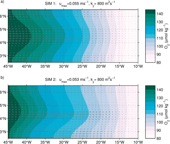
Kamenkovich et al., 2009). Brandt et al. (2010) found thatky = 200m2/s andkx = 2.5×ky(kxis the zonal diffusivity) best fits the observations in the ETNA OMZ (∼400 m depth). Here we calculate the equilibrium state for differentkyandkx. We found that a meridional eddy diffusivity ofky = 800m2/s with no anisotropy (i.e.,kx = ky) andu0 = 0.055m/s results in oxygen concentrations along 23◦W that best matches observa- tions (Figures S1a and S1c in the supporting information). In the following, we will refer to this simulation as SIM 1.
3. Results
The interannual variability of the NEUC and its impact on the oceanic oxygen distribution are investi- gated using ship observations along 23◦W and the output of TRATL01. First we briefly validate and discuss the zonal velocity and oxygen sections along 23◦W TRATL01. Then we present the results of the inter- annual variability of the NEUC in TRATL01 before we focus on the oxygen response associated with NEUC variability. Finally, we present the results of the conceptual model to understand the role of specific mechanisms.
Table 2
NEUC INT ( Sv), YCM(◦N) and Oxygen (𝜇mol/kg) Derived From Observations Along 23◦W From 2002 to 2018
Date YCM INT (i) O2 (ii) O2 AMM
2002 Oct 4.38 1.73 ◦
2003 Aug 4.79 4.93 ◦
2006 Jun 5.36 0.76 107.2 106.5 ◦
2006 Jun 5.22 1.02 108.5 108.9 ◦
2006 Jun 4.95 0.84 111.9 109.2 ◦
2008 Mar 5.41 0.83 105.2 104.8 ◦
2008 Mar 5.53 0.72 ◦
2009 Jul 5.25 1.83 −
2009 Nov 4.47 2.42 106.1 103.7 −
2009 Nov 4.63 3.07 −
2010 Feb 4.60 2.84 +
2010 May 5.02 6.91 +
2011 May 4.96 0.08 ◦
2011 Aug 5.24 5.83 ◦
2012 Nov 5.12 2.02 98.1 96.6 ◦
2012 Nov 4.83 1.51 ◦
2014 May 4.71 4.15 96.5 100.8 −
2014 Nov 4.76 3.45 104.7 104.5 −
2015 Sep 5.60 1.25 114.1 115.4 −
2016 Aug 4.49 2.10 110.0 108.1 ◦
2018 Feb 4.74 5.80 108.5 107.2 −
total mean single sections 4.96±0.08 2.58±0.42 107.1±1.8 106.0±1.5
mean section (2002-2018) 4.84 1.36 107.7 106.1
Note. NEUC = North Equatorial Undercurrent; AMM = Atlantic meridional mode. The oxygen values are derived in two ways. (i) The values are average in a meridionally varying frame (100- to 300-m depth,(YCM− 1.5)◦-(YCM +1)◦N). (ii) The values are averaged in a fixed box (100 to 300 m depth, 3◦–6.5◦N). The state of the AMM is marked for positive events (+), negative events (−), and neutral phases (◦). For the mean values derived from the single ship sections, the standard error is given.
3.1. Mean Velocity and Oxygen Section Along 23◦W
In the mean ship section along 23◦W, below the mixed layer, higher oxygen concentrations locally coincide with the eastward-flowing EUC, NEUC, and nNECC at 0◦N, 4.5◦N, and 8.5◦N, respectively, whereas the westward flows centered at 2.5◦N and 6.5◦N are associated with lower oxygen concentrations (Figures 2a and 2c). The core of the ETNA OMZ with oxygen concentrations of 40𝜇mol/kg is located between 400 and 500 m and between 9◦N and 13◦N. In the upper 250 m south of 6◦N, oxygen concentration are in general higher than north of 6◦N. This is associated with the more energetic zonal flow in the near-equatorial belt including the NEUC.
From the observed zonal velocity field the NEUC intensity (INT, equation (2)) and central position (YCM, equation (1)) are calculated and averaged in two different ways: (i) They are calculated using the mean ship section. Here the averaged NEUC intensity is 1.2 Sv, and the current is on average located at 4.9◦N. (ii) The estimates of the single ship sections are averaged. This results in an average intensity of 2.6 ± 0.4Sv and an averaged central position of 5.0± 0.1◦N (Table 2). Method (ii), which results in higher values, is more consistent with the method used for the model output.
Similar to the observations, oxygen concentrations along 23◦W in TRATL01 are increased in the presence of eastward flow and decreased in the presence of westward flow (Figures 2b and 2d). The NEUC in TRALT01 is on average more than twice as strong as in the observations, and its core is located a bit further south. The mean NEUC intensity at 23◦N (1990–2007) is 7.4±0.3Sv, and its mean central position is 4.44±0.03◦N. The model is overestimating the strength and depth range of the NEUC and the nSEC whereas weaker eastward current bands such as the NICC and the nNECC are not well represented by the model.
In TRATL01 oxygen concentrations below the mixed layer are generally lower, the OMZ is located shallower, and the difference between local oxygen maxima and minima is smaller compared to observations. The core of the OMZ in TRATL01 is 200 m shallower than in observations. Also, the deep oxygen maximum at the equator is not well represented in TRATL01. Although the NEUC is stronger, oxygen concentrations within the NEUC region at 23◦W (100 to 300 m depth, 3◦–6.5◦N) are lower in TRATL01 (93.4 ± 0.8𝜇mol/kg) compared to observations (106.0± 1.5𝜇mol/kg).
Different mechanisms seem to dominate the NEUC mean state in observations and in TRATL01. Not only the NEUC is very strong in TRALT01 but also the nSEC south of it. One explanation for that can be a too strong recirculation between nSEC and NEUC. In the ship section from February 2018, a temporary recircu- lation between the nSEC and NEUC seems to exist (black dashed rectangles in Figures 1b and 1c). Here the velocity maximum between 3◦N and 5◦N in the depth range of 50 to 300 m is associated with rather low oxy- gen, and it is located above and south of the NEUC associated oxygen maximum. It is likely that this eastward velocity maximum is a temporary recirculation of the nSEC, which overlaps with the actual NEUC flow.
This results in lower oxygen values associated with higher eastward NEUC velocities. An overestimation of this process by TRATL01 could result in the shown discrepancies between model and observations. Strong recirculation between EUC, NEUC, and nSEC are also shown in other model studies such as Hüttl-Kabus and Böning (2008).
In summary, distinct discrepancies exist between simulated and observed zonal velocities and oxygen con- centration in the mean sections along 23◦W. A potential cause for the differences in the mean state is an overestimation of the recirculation between nSEC and NEUC in TRATL01. Nevertheless, we want to emphasize here that the horizontal oxygen distribution is clearly improved in TRATL01 compared to coarser resolution models (Duteil et al., 2014). How the erroneous representation of the mean state in TRATL01 affects the NEUC and associated oxygen changes on interannual time scales will be investigated in section 3.4. Before we focus on the oxygen response to the NEUC we investigate the variability of NEUC transports and central position. In the next section we briefly study the seasonal cycle of the NEUC in observations and in TRATL01.
3.2. Seasonal Cycle of NEUC Intensity (INT) and Central Position (YCM)
In the previous section we found that on average the NEUC is too strong in TRATL01 but simultaneously shows a weaker oxygen maximum along 23◦W compared to observations. We hypothesize that this might be due to an overestimation of the recirculations between nSEC and NEUC in TRALT01. Here we focus on the seasonal cycle of the NEUC in observations and in TRATL01.
The NEUC transport estimates derived from the observational data are highly variable and show no clear seasonal signal (Table 2 and black dots in Figure 3a). This is in agreement with previous observational results (Bourlès et al., 2002, 1999; Brandt et al., 2006; Schott et al., 1995, 2003; Urbano et al., 2008). The current is weak and likely to be obscured by mesoscale activities (e.g., Goes et al., 2013; Weisberg & Weingartner, 1988) and interannual variability (Goes et al., 2013; Hüttl-Kabus & Böning, 2008). Even with this unique data set of 21 ship sections, observations are still too sparse to identify a seasonal variability of the NEUC.
In TRATL01, the NEUC shows a clear seasonal cycle. Along 23◦W, the NEUC reaches its maximum inten- sity of 11.4 Sv in May and its minimum intensity of 3.9 Sv in November (red line in Figure 3a). Its central position shows a semiannual cycle with southernmost positions in September and January and northern- most positions in May and November (Figure 3b). The semiannual cycle of NEUC central position is not visible at all longitudes (Figure 3d). The seasonal signal of NEUCINTandYCMis propagating from the east- ern boundary toward the west (Figures 3c and 3d). Highest standard deviations of NEUC transports occur during May and June in the eastern basin and during July and August in the western basin (black contours in Figure 3c). Maximum standard deviation of NEUC transports seems to be associated with the seasonal weakening of the NEUC.
The seasonal cycle of the NEUC in TRATL01 generelly agrees with previous studies. Hüttl-Kabus and Bön- ing (2008) also found a more northward position and higher transports between April and August and a more southward position and lower transports between September and March in their model simulation.
The seasonal cycle of NEUC transport estimates in TRATL01 is also consistent with the synthesis product of Goes et al. (2013). Similar to Goes et al. (2013), we found a semiannual cycle of the NEUC central position
Figure 3.Seasonal cycle of (a) North Equatorial Undercurrent (NEUC) intensity (INT) and (b) NEUC central position (YCM) at 23◦W derived from TRATL01 (red lines, 1958–2007) as well as NEUCINTderived from each ship section (black dots in a; circles, squares, and crosses mark years of neutral, negative, and positive Atlantic Meridional Mode phases, respectively). The red bars denote the standard deviations of NEUCINTandYCMin TRALT01 of the respective months from 1958 to 2007. Hovmöller diagram of the 1958–2007 seasonal cycle of (c)INTand (d)YCMin TRATL01 for each longitude. The black contours show the standard deviation of (c)INTin Sv and (d)YCMin degree latitude for each month from 1958 to 2007.
along 23◦W, although the timing of maxima and minima is shifted by up to 2 months. We found minima in September and January and maxima in May and November, whereas in Goes et al. (2013) minima occur in September and March and maxima in August and December. In general, the seasonal strengthening of the eastern NEUC in TRATL01 seems to coincide with the northward migration of the Intertrop- ical Convergence Zone (ITCZ) and the shoaling of the thermocline in the eastern equatorial Atlantic (Xie & Carton, 2004).
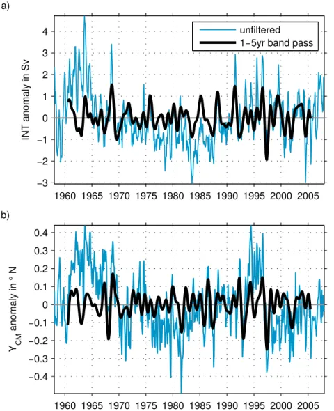
Figure 4.Zonally averaged (42◦–15◦W) monthly mean anomaly of (a) North Equatorial UndercurrentINT (equation (2)) and (b)YCM(equation (1)) with respect to the 1958–2007 seasonal cycle estimated from TRATL01. A 1- to 5-year band-pass (black line) Butterworth filter is applied to the zonally averaged time series (blue lines).
In summary, a seasonal and longer-term variability of the NEUC in observations cannot be identified. In TRATL01 the NEUC shows a clear seasonal cycle that is in general agreement with previous studies. This encourages us to study the interannual variability of the NEUC in the next section.
3.3. Interannual Variability of the NEUC
The NEUC transport and central position vary on interannual to multidecadal time scale in TRATL01 (Figure 4). However, TRATL01 is driven by CORE v2 wind forcing that is based on NCEP winds. The CORE forcing as well as the NCEP wind is known to exhibit spurious multidecadal wind variability (Fiorino, 2000;
He et al., 2016; Hurrell & Trenberth, 1998). We therefore focus on the interannual variability of the NEUC in TRATL01.
NEUC transport and central position show a positive correlation in TRATL01. To analyze the correlation, we zonally averaged NEUCINTandYCMfrom 42◦W to 15◦W and removed the seasonal cycle from 1958 to 2007 (blue lines in Figure 4). To better understand the role of interannual variability of the NEUC, we applied a 1- to 5-year band-pass Butterworth filter toINTandYCM(black lines in Figure 4). Higher NEUC transports are generally associated with a more northward position of the NEUC and vice versa with a significant positive correlation between the band-pass filtered time series ofR = 0.33.
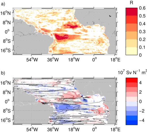
Figure 5.Linear regression of 1- to 5-year band-pass filtered North Equatorial UndercurrentINTonto wind stress curl from TRATL01. (a) Coefficient of correlation and (b) slope of the linear regression. Contours in (b) present the anomalous Sverdrup circulation forced by a wind stress curl anomaly that causes a North Equatorial Undercurrent transport anomaly of 1 Sv. The black solid lines mark the 0, 0.1, 0.4, and 1 Sv isoline and the black dashed lines mark the−0.1,−0.4, and−1 Sv isoline.
Previous studies suggest the upwelling in the Guinea Dome and along the Northwest African coast in the ETNA as a possible driver of the NEUC (Furue et al., 2007, 2009) and that changes in the wind field can impact the upwelling, which in turn leads to changes in the NEUC (Goes et al., 2013). To investigate this connection, we perform a linear regression of the band-pass filtered NEUCINTonto the wind stress curl using monthly time series regressed at lag 0 (Figure 5). On interannual time scales, the wind stress curl explains up to 40% of the NEUC variability. Maximum positive correlation (R = 0.6) is found in the eastern basin of the tropical North Atlantic between 2◦N and 8◦N and in the western basin of the tropical South Atlantic between 0◦and 8◦S. This large-scale wind pattern may not only impact the strength of the NEUC but also effect the basin-wide circulation. We therefore regressed the wind stress curl on the NEUC and calculate the anomalous Sverdrup streamfunction from the derived slopebtimes a unit transport of 1 Sv.
During a strong (weak) NEUC, the derived anomalous Sverdrup streamfunction is associated with a west- ward (eastward) velocity anomaly between 8◦N and 10◦N and an eastward (westward) velocity anomaly just south off the equator (Figure 5). At the western boundary the closure of the anomalous Sverdrup stream- function would result in a southward (northward) and northward (southward) velocity anomaly north and south of the equator, respectively. Between 40◦W and 10◦W just north of the equator the wind stress curl anomaly leads to an anomalous northward (southward) Sverdrup transport. To further investigate the rela- tionship between the NEUC and the large-scale wind field, we perform a composite analysis regarding the wind and SST field during strong and weak NEUC transports.
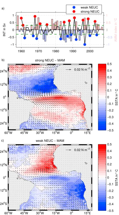
The band-pass filtered time series of NEUCINTis used to define years of strong and weak NEUC flow. As threshold 0.6 times its standard deviation is chosen (green line in Figure 6a). Then composites of SST and the wind field are calculated for years of strong and weak NEUC transports (Figures 6b and 6c). The composites show an interhemispheric SST gradient with opposite sign for strong and weak NEUC transports. Associated
Figure 6.(a) Annual mean of North Equatorial Undercurrent (NEUC)INTanomaly averaged between 42◦W and 14◦W. A 1- to 5-year band-pass filter is applied to the time series (lefty-axis). The green dashed line marked±0.6times the standard deviation of the time series. Red dots mark years of strong NEUCINT; blue dots mark years of weak NEUCINT. The bars show the March to May (MAM) averages of the Atlantic meridional mode (AMM) index after Servain (1991) (righty-axis). Composites of anomalous sea surface temperature (SST; color shading) and surface wind stress (arrows) for years of (b) strong and (c) weak NEUCINT.
are wind anomalies pointing from the colder hemisphere toward the warmer hemisphere. These are the characteristics of the AMM as described in the introduction. The interannual NEUC variability is negatively correlated with the AMM. A positive AMM is associated with a weaker and more southern NEUC, and the negative AMM is associated with a stronger and more northern NEUC.
The anomalous interhemispheric winds during an AMM event link the interannual variability of the NEUC to the AMM. Associated with a positive (negative) AMM event is a negative (positive) wind stress curl anomaly along the equator and just north of it east of 20◦W (Foltz & McPhaden, 2010b; Joyce et al., 2009).
We find a similar wind pattern for weak and strong NEUC, respectively (Figure 5). The large-scale wind pat- tern does not only affect the NEUC flow but also affects the basin-wide Sverdrup circulation in the tropical Atlantic (Figure 5). The anomalous northward Sverdrup transport between 40◦W and 10◦W just north of the equator might impact the recirculation between the NEUC and the nSEC. Furthermore, along the North- west African coast south of 15◦N, we find alongshore wind stress that act to weaken (strengthen) coastal upwelling during weak (strong) NEUC transports (Figure 6).
In summary, in TRATL01 the interannual variability of the NEUC is linked to the AMM, likely due to its asso- ciated large-scale wind anomalies. Consistent with the results of Goes et al. (2013), we find a strengthening and a more northward position of the NEUC during negative AMM events and vice versa. The anoma- lous wind stress curl additionally impacts the Sverdrup circulation between 10◦S and 10◦N. The response of oxygen to the interannual changes of the NEUC in TRATL01 is investigated in the next section.
3.4. NEUC Impact on Oxygen
On interannual time scales the NEUC variability is linked to the AMM in TRATL01. During positive AMM events, the NEUC transports are weaker, and the current core is displaced toward the south. During negative AMM events, the NEUC is stronger and displaced toward the north. In this section we investigate the impact of the interannual NEUC variability on oxygen. Brandt et al. (2010) suggest that weaker NEUC transports lead to lower oxygen concentrations at 23◦W due to a weaker advection of oxygen-rich water masses from the western boundary. Consequently, we expect lower oxygen concentrations after positive AMM events and vice versa. The observational data show no clear connection between oxygen concentration, NEUC transports, and the AMM (Figure S2). We will therefore focus on the interannual variability of oxygen in TRATL01.
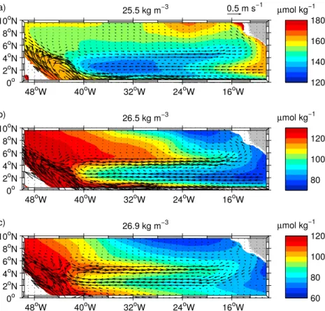
In TRATL01 the oxygen variability is analyzed along three characteristic neutral density (𝛾n) surfaces of the NEUC. We choose the 25.5 kg/m3surface for the upper part of the NEUC, the 26.5 kg/m3surface for the central part of the NEUC, and the 26.9 kg/m3surface for the lower part of the NEUC (Figure 2). The mean oxygen concentrations and horizontal velocities along all three𝛾nsurfaces of the period 1990 to 2007 are shown in Figure 7. Along the upper𝛾nsurface in the area of the nSEC and NEUC low oxygen concentrations exist (Figure 7a). Interestingly, minimum oxygen concentrations are found in the western basin in the area of the nSEC supplying the eastward flow within the NEUC. This suggests that the water masses in the upper NEUC in TRATL01 are only weakly connected to the oxygen-rich waters in the western boundary and are instead provided largely out of the recirculation between NEUC and nSEC. A possible mechanism causing the low-oxygen values along the 25.5 kg/m3surface close to the western boundary might be a too weak or inexistent intermediate current system in TRATL01. This would lead to a too low ventilation at depth, which again can result in an upward flux of low-oxygen waters toward the surface due to either diapycnal mixing or vertical advection within the subthermocline cells (Perez et al., 2014; Wang, 2005).
Along the 26.5 kg/m3surface oxygen concentrations are high in the western basin and low in the eastern basin (Figure 7b). At the northern flank of the NEUC and north of it a tongue of high oxygen concentrations spreads toward the east. At the southern flank of the NEUC and within the nSEC a tongue of low oxygen spreads toward the west. The mean horizontal current field in combination with the oxygen concentrations indicates that the NEUC in TRATL01 is partly supplied by water masses from the western boundary and partly by water masses from the nSEC. This supports our previous hypothesis that in TRATL01 a constant recirculation between nSEC and NEUC superimposed on a mean eastward current results in a strong NEUC flow that is associated with low oxygen levels, as it is supplied by the oxygen-poor water masses out of the nSEC.
At the lower part of the NEUC (26.9-kg/m3surface) a tongue of high oxygen concentration centered at the NEUC spreads from the western to the eastern basin (Figure 7c). Here the ventilation of the NEUC by the
Figure 7.Mean oxygen concentration (shading) and horizontal velocities (arrows) for the period 1990 to 2007 along three characteristic isopycnals (25.5, 26.5, and 26.9 kg/m3) of the North Equatorial Undercurrent in TRALT01.
western boundary seems to dominate the water supply of the NEUC with only weak recirculation occurring along the eastward path of the NEUC. Note that eastward flow of waters with higher oxygen concentrations associated with the NEUC reaches the eastern boundary north of 6◦N.
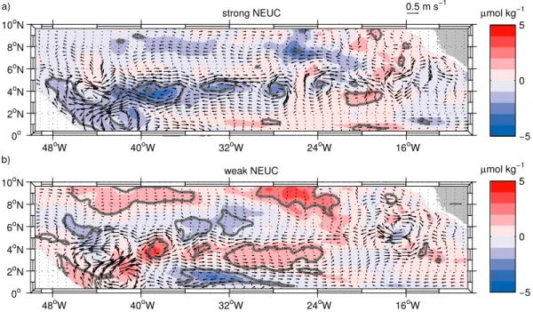
To investigate interannual variability of oxygen in TRATL01, the seasonal cycle is removed from the oxygen field, and a 5-year high-pass Butterworth filter is applied to the annual averaged oxygen anomalies. Similar to the SST and wind stress analysis, composites of oxygen and horizontal velocity for strong and weak NEUC transports are calculated (Figure 8). We now focus on the oxygen variability along the 26.5 kg/m3surface representing the core depth of the NEUC in TRATL01.
At a first glance, the oxygen anomalies associated with the NEUC variability in TRATL01 appear to be coun- terintuitive. Along the 26.5-isopycnal during years of weak NEUC, positive oxygen anomalies exist along the NEUC path with a connection to the southwestern boundary (Figure 8a). For years of strong NEUC flow, negative oxygen anomalies occur along the NEUC path instead (Figure 8b). This is the opposite of what we would have expected taken into account the mean velocity and oxygen fields along 23◦W.
Again, a too strong recirculation between the nSEC and NEUC might explain the oxygen pattern in TRALT01. The composite analysis shows that during weak (strong) NEUC flow, also, the nSEC is weak (strong) and is transporting less (more) oxygen-poor water to the western basin (Figure 8). Associated is a weaker (stronger) than normal recirculation between NEUC and nSEC, and the NEUC is supplied by less (more) oxygen-poor water from the nSEC. Additionally a weak (strong) nSEC is transporting less (more) oxygen-poor water to the western basin. Positive (negative) oxygen anomalies develop in the western basin, which may be then advected by the NEUC toward the east.
In the oxygen composites, anomalies occur in the entire tropical North Atlantic, which might be associ- ated with the detected large-scale wind anomalies during anomalous NEUC transports. For example, weak negative (positive) oxygen anomalies exist along the western boundary during strong (weak) NEUC phases and cover a depth range of 50 to 450 m depth. These oxygen anomalies are associated with weak merid- ional velocity anomalies that act to weaken (strengthen) the NBC and its return flow. This pattern could be
Figure 8.Anomalous oxygen concentrations (shading) and horizontal velocities (arrows) for years of strong (a) and weak (b) North Equatorial Undercurrent (NEUC) flow along the 26.5 kg/m3-isopycnal in TRATL01. The annual mean data were 5-year high-pass filtered. Areas within the gray contour lines mark oxygen anomalies that are significant at a 95% confidence level.
related to the closure of the Sverdrup circulation at the western boundary (Figure 5b). The wind field during strong (weak) NEUC and negative (positive) AMM events acts to weaken (strengthen) the NBC just north of the equator so that less (more) oxygen-rich water might be supplied there. Furthermore, negative (pos- itive) oxygen anomalies during strong (weak) NEUC flow exist also north of 7◦N. Here we find westward (eastward) velocity anomalies in the anomalous Sverdrup streamfunction at about 8◦N that are also visible in Figure 8. This westward (eastward) velocity anomaly act to weaken (strengthen) the nNECC, which again could explain the oxygen anomalies there.
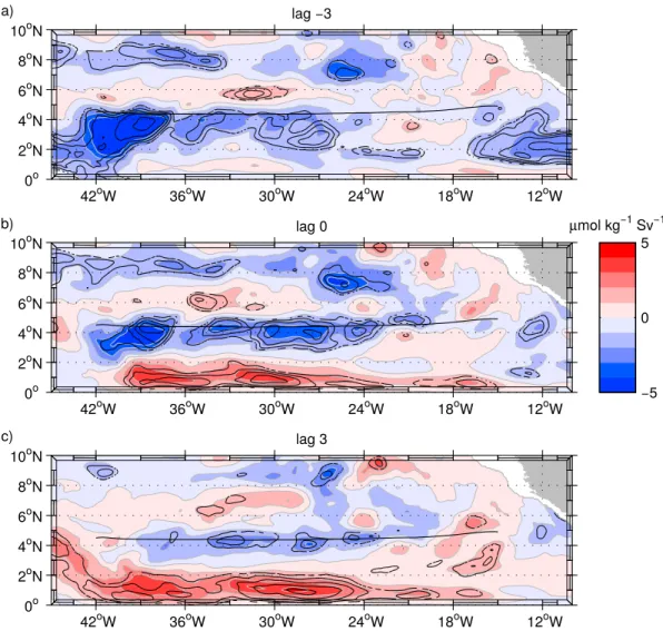
In contrast to our expectations, the NEUC strength and the oxygen concentrations along its flow path are negatively correlated on interannual time scales in TRATL01. To get a rough estimate of how much of the oxygen variability can be explained by the NEUC variability, we perform a lagged linear regression of oxygen on NEUC INT for the 1- to 5-year band-pass filtered time series (Figure 9). The linear regression supports the results from the composite analysis, that is, a negative correlation between oxygen and NEUC in TRATL01 (Figure 9). Highest values of R occur along and slightly south of the NEUC pathway mainly between 42◦W and 24◦W (Figures 9a–9d). Here on average the NEUC variability can explain between 20% and 40% of the oxygen variability. MaximumRvalues occur just south of the NEUC west of 36◦W when the NEUC leads the oxygen by 3 months. This hints again toward the relationship between nSEC and NEUC. If the nSEC is weak, less oxygen-poor water is transported toward the west, leading to a positive oxygen anomaly there that is maximum 3 months after nSEC is weakest. Striking is also the high correlation near the equator in Figure 9e, suggesting that the oxygen variability there leads the NEUC variability further north. A possible explanation might be that the variability of the near-equatorial flow is leading the variability of the NEUC.
A lead-lag correlation between NEUCINTand the zonal velocity shows eastward velocity anomalies along the equator leading an anomalous strong NEUC by 3 months, but the correlation is low.
We here want to briefly discuss the role of respiration for oxygen variability. Generally, respiration can be another mechanism changing the oxygen concentration. However, on interannual time scales the variability of respiration in TRATL01 is too small to have a significant effect on oxygen. This is consistent with other studies showing that circulation changes are the dominant mechanism setting the variability of oxygen levels on seasonal and multidecadal time scales (Montes et al., 2014; Pozo Buil & Di Lorenzo, 2017; Vergara et al., 2016; Yang et al., 2017).
Figure 9.Linear regression of TRATL01 oxygen concentrations along the 26.5 kg/m3-isopycnal on North Equatorial Undercurrent (NEUC)INT. Shading marks the slope of linear regression for a lag of−3 months (a; NEUC leads oxygen), zero lag (b), and a lag of +3 months (c; oxygen leads NEUC). Negative values of the slope indicate an anticorrelation between NEUC and oxygen; that is, oxygen is low when the NEUC transport is strong. Black contours mark the significant values of the coefficient of determination (0.1 interval starting at 0.4). Black line marks mean position of the NEUC.
In summary, NEUC transports and oxygen concentrations along its pathways are anticorrelated on interan- nual time scales in TRATL01. This is in contrast to the conclusion drawn from observations (Brandt et al., 2010), where a stronger NEUC is associated with higher oxygen concentrations. The results of this section motivates us to four experiments with a conceptual model that are described in the next section.
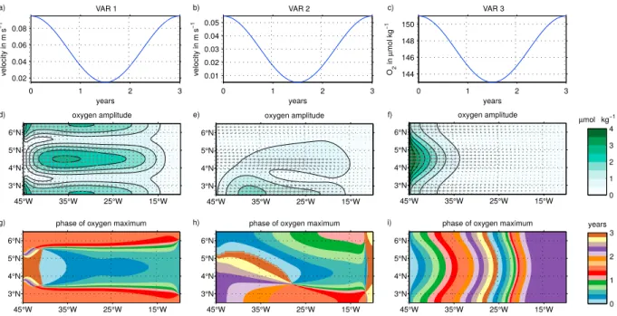
3.5. Conceptual Model
The conceptual model is used to investigated single processes that appear to be active in the observations and/or in TRATL01. These processes potentially impact the NEUC, its variability, and the associated oxygen distribution. In addition to our reference experiment SIM 1, we perform four experiments (SIM 2 and VAR 1-3) with the conceptual model. First, we want to test how a mean recirculation between NEUC and nSEC affect the oxygen concentrations (SIM 2). Furthermore, we calculate the oxygen response for three possible scenarios: (i) a stronger mean NEUC that is associated with enhanced ventilation from the western boundary and, hence, positive oxygen anomalies along the NEUC (VAR 1); (ii) a stronger NEUC due to a stronger recirculation with the nSEC, which is associated with negative oxygen anomalies in the NEUC (VAR 2); (iii) an oxygen variability of the source waters at the western boundary, which is then advected by the unchanged NEUC toward the east (VAR 3). The experiments are based on the conceptual model (equation (3)) with the horizontal eddy diffusivitieskx = ky = 800m2/s and the background flow field given by equation (4) with