Inès N. Otosaka1 , Andrew Shepherd1 , Tânia G. D. Casal2, Alex Coccia3, Malcolm Davidson2, Alessandro Di Bella4 , Xavier Fettweis5 , René Forsberg4 , Veit Helm6 , Anna E. Hogg7 , Sine M. Hvidegaard4 , Adriano Lemos1,8 , Karlus Macedo3, Peter Kuipers Munneke9 , Tommaso Parrinello10, Sebastian B. Simonsen4 , Henriette Skourup4 ,
and Louise Sandberg Sørensen4
1Centre for Polar Observation and Modelling, School of Earth and Environment, University of Leeds, Leeds, UK,
2ESA‐ESTEC, Noordwijk, The Netherlands,3Metasensing, Noordwijk, The Netherlands,4Technical University of Denmark, DTU Space, Lyngby, Denmark,5University of Liège, Liège, Belgium,6Alfred Wegener Institute, Helmholtz Centre for Polar and Marine Research, Bremerhaven, Germany,7School of Earth and Environment, University of Leeds, Leeds, UK,8Now at University of Gothenburg, Göteborg, Sweden,9Institute for Marine and Atmospheric Research Utrecht, Utrecht University, Utrecht, The Netherlands,10ESA‐ESRIN, Frascati, Italy
Abstract
Greenland Ice Sheet surface melting has increased since the 1990s, affecting the rheology and scattering properties of the near‐surfacefirn. We combinefirn cores and modeledfirn densities with 7 years of CryoVEx airborne Ku‐band (13.5 GHz) radar profiles to quantify the impact of melting on microwave radar penetration in West Central Greenland. Although annual layers are present in the Ku‐band radar profiles to depths up to 15 m below the ice sheet surface,fluctuations in summer melting strongly affect the degree of radar penetration. The extreme melting in 2012, for example, caused an abrupt 6.2 ± 2.4 m decrease in Ku‐band radar penetration. Nevertheless, retracking the radar echoes mitigates this effect, producing surface heights that agree to within 13.9 cm of coincident airborne laser measurements. We also examine 2 years of Ka‐band (34.5 GHz) airborne radar data and show that the degree of penetration is half that of coincident Ku‐band.Plain Language Summary
Radar waves emitted by satellites can be used to measure changes in surface elevation of the Greenland Ice Sheet. However, they do not reflect off the ice sheet surface itself but penetrate into the snow to a depth of about 15 m for radar wavelengths of 2.3 cm. When the snow melts, meltwater can percolate into the snow or refreeze at the surface. Layers of refrozen ice sharply reduce the degree of radar penetration and may be mistaken for an elevation increase in radar measurements. Here, we combinefirn cores and modeledfirn densities with 7 years of airborne radar data collected duringfield campaigns in West Central Greenland to quantify this effect. We identify internal layers corresponding to annual stratigraphy within the snowpack, and we show that more melt means less radar penetration into the firn. The unprecedented surface melting which occurred across Greenland in 2012 caused a sharp reduction in the degree of radar penetration, from 11.5 to 5.3 m. However, if the effects of penetration are corrected for, radar altimeters can accurately measure the surface elevation of the ice sheet.1. Introduction
In recent decades, increased melting at the surface of the Greenland Ice Sheet (van den Broeke et al., 2016) has had a marked impact on rates of runoff (Enderlin et al., 2014; van Angelen et al., 2014) and glacierflow (van de Wal et al., 2008), and has also affected the structure of the near‐surfacefirn owing to the redistribu- tion and refreezing of surface meltwater (de la Peña et al., 2015; Machguth et al., 2016). These processes, and the associated changes infirn properties, present challenges for satellite radar altimetry surveys of the ice sheet mass balance when converting observations of volume change to mass change (McMillan et al., 2016).
Surface melting has a large impact on thefirn stratigraphy and density as meltwater can refreeze at the sur- face, or percolate into the snowpack and refreeze to form ice lenses (Benson, 1996), or refreeze in between already existing ice layers and form thicker ice slabs (MacFerrin et al., 2019). Ice cores provide records of density and stratigraphy at point locations (Mosley‐Thompson et al., 2001) andfirn densification models provide estimates of densities across the ice sheet (e.g., Kuipers Munneke et al., 2015). Radars have also
©2020. The Authors.
This is an open access article under the terms of the Creative Commons Attribution License, which permits use, distribution and reproduction in any medium, provided the original work is properly cited.
Key Points:
• We use airborne radar,firn cores, andfirn models to confirm that summer melting is the principal source of radar penetration fluctuations
• The largestfluctuations are recorded after the extreme melt event of 2012, which caused a 6.2 ± 2.4 m reduction in radar penetration
• Echo retracking compensates for radar penetrationfluctuations, leading to surface heights that agree with laser data to within 13.9 cm
Supporting Information:
• Supporting Information S1
• Data Set S1
Correspondence to:
I. N. Otosaka, eeino@leeds.ac.uk
Citation:
Otosaka, I. N., Shepherd, A., Casal, T. G. D., Coccia, A.,
Davidson, M., Di Bella, A., et al. (2020).
Surface melting drivesfluctuations in airborne radar penetration in West Central Greenland.Geophysical Research Letters,47, e2020GL088293.
https://doi.org/10.1029/2020GL088293
Received 10 APR 2020 Accepted 7 AUG 2020
Accepted article online 21 AUG 2020
been widely used over glaciers and ice sheets to map their structure (MacGregor et al., 2015), calculate accu- mulation rates (Miège et al., 2017), and track changes in their elevation (Shepherd et al., 2019).
Radar systems transmit electromagnetic pulses and record the amplitude and time delay of the waves scat- tered back from discontinuities in the dielectric properties. Their echoes are sensitive to density variations in thefirn column, and thefirn structure can reveal continuous internal scattering horizons, corresponding to isochrones (Hawley et al., 2006). Both ground‐based (Brown et al., 2012) and airborne radar, such as the snow radar flown during NASA Operation IceBridge (Koenig et al., 2016; Medley et al., 2013;
Montgomery et al., 2020) or the European Space Agency's Airborne SAR/Interferometric Radar Altimeter System (ASIRAS) operating at Ku‐band (de la Peña et al., 2010; Helm et al., 2007; Overly et al., 2016;
Simonsen et al., 2013), have been used to track isochrones and derive accumulation rates. Unlike ground‐based and airborne radar, satellite radar measurements lack the vertical resolution to resolve the internal structure of thefirn column due to the smaller bandwidth and coarser spatial resolution of the radar footprint. Nonetheless, satellite radar altimeters are sensitive to variations in thefirn properties as the radar signal penetrates into the snowpack. Additionally, the radar signal penetration is frequency dependent. At present, two frequencies are used by satellite radar altimeters: Ku‐band (13.5 GHz) is used by CryoSat‐2 and Sentinel 3A/B, and Ka‐band (37 GHz) is used by AltiKa. Studies have shown that at Ku‐band, the radar signals can penetrate up to ~15 m intofirn, while the penetration depth of higher‐frequency Ka‐band radars is reduced to ~0.5 m (Rémy et al., 2015). The altimeter echo recorded is therefore a combination of surface and volume scattering (Ridley & Partington, 1988). The ratio between surface and volume scattering varies spatially and temporally according to changes in the surface and subsurface properties and may impact the height retrieval from radar altimeters (Simonsen & Sørensen, 2017).
In this study, we use airborne Ku‐band radar data acquired using the ASIRAS instrument, Ka‐band radar data acquired using the KAREN radar (the MetaSensing Ka‐band altimeter), airborne laser data, shallow firn cores (< 6 m), andfirn density models to characterize and assess the impact of spatial and temporalfluc- tuations in the properties of the near‐surfacefirn in West Central Greenland. This study is performed along the glaciological transect established during the Expéditions Glaciologiques Internationales au Groenland (EGIG) in 1958 (Renaud et al., 1963). The EGIG line extends from the ablation zone at the Western margin of the ice sheet, across the percolation and dry snow zones to the Summit, and further toward the Eastern margin and is therefore a representative location of density variations across the Greenland Ice Sheet (Parry et al., 2007).
2. Data and Methods
The EGIG line (Figure 1a) has been surveyed for more than a decade as part of ESA's Cryosat Validation Experiment (CryoVEx). According to previous in situ investigations of snow density and stratigraphy, EGIG line sites T3 to T21 lie in the percolation zone with site T21 marking the start of the dry snow zone (Morris & Wingham, 2011; Scott et al., 2006). In this study, we use data collected between 2006 and 2017 over a ~675 km transect of the EGIG line, starting about 14 km from Ilullissat airport at an elevation of 157 m above sea level (m.a.s.l.), 115 km before site T1, and ending 149 km beyond site T41 at an altitude of 2,956 m.a.s.l.
Shallowfirn cores were collected in October 2016 (T1, T4, and T5) and April 2017 (T5, T9, T12, T19, T30, and T41) (Table S1 in the supporting information). The stratigraphy was recorded by illuminating the cores to identify ice lenses. Firn density was measured by weighing the different stratigraphic layers (see Supporting Information S1). These in situ density measurements are used to evaluate twofirn densification models: (1) the stand‐alone Institute for Marine and Atmospheric Research Utrechtfirn densification model (IMAU‐FDM) (Ligtenberg et al., 2011, 2018), forced at the surface by RACMO (Noël et al., 2018).
IMAU‐FDM simulates the density and temperature in a vertical, one‐dimensionalfirn column through time at a vertical resolution of 5 cm and (2) the CROCUS snow model (Brun et al., 1992) embedded in the Modèle Atmosphérique Régional (MAR) (version 3.10, Fettweis et al., 2017, 2020) to derive the MARfirn densifica- tion model (MAR‐FDM). CROCUS simulates the transfer of mass and energy between afixed number of layers of snow,firn, or ice with a vertical resolution varying from 5 to 500 cm.
Airborne radar data were collected in 2004, 2006, 2008, 2011, 2012, 2014, 2016, and 2017, along segments of the EGIG line of varying length. For all CryoVEx airborne surveys, the same aircraft and instrumental setup
10.1029/2020GL088293
Geophysical Research Letters
were used, which includes an airborne laser scanner (ALS), the ASIRAS radar, and the KAREN radar in two surveys in 2016 and 2017. The ALS is a Riegl LMS‐Q140‐i60 laser scanner operating at 904 nm (red), which gives surface heights in 0.7 m intervals across a 300‐m‐wide swath with an accuracy of 0.1 m (Skourup et al., 2019). ASIRAS is a Ku‐band radar designed as a prototype for the SIRAL altimeter on board CryoSat‐2 operating at a central frequency of 13.5 GHz with a bandwidth of 1.0 GHz, range resolution of 0.109 m in air, and a nominal footprint size of 10 m across‐track and 3 m along‐track at aflight elevation of ~300 m a.g.l. (Cullen, 2010). KAREN is a Ka‐band radar altimeter operating at a central frequency of 34.5 GHz—the same frequency used by AltiKa—with a bandwidth of ~0.5 GHz, range resolution of 0.165 m in air, and a footprint size of 10 m across‐track and 5 m along‐track (version “levc”). Data acquired when the aircraft roll angle exceeded ±1.5° were discarded.
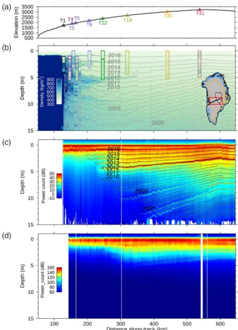
Figure 1.(a) Elevation profile along the EGIG line. (b) IMAU‐FDM density profile (31/03/2017) andfirn core densities.
The isochrones traced from IMAU‐FDM are indicated by gray lines. Thefirn cores from 2016 are offset by the net SMB relative to 2017. The inset shows the location of the study area. (c) ASIRAS Ku‐band radar profile. The traced layers are indicated by black lines. (d) KAREN Ka‐band radar profile. The two radar profiles were acquired on 31/03/2017 and 01/04/2017. Along‐track distance is relative to Ilulissat airport.
We applied three different retracking algorithms to locate the ice sheet surface in the radar echoes as differ- ent processing strategies have been shown to affect the elevation measurements when the radar penetration depth varies (Slater et al., 2019). We used (1) an offset center of gravity (OCOG) retracker (Wingham et al., 1986), (2) a 30% threshold center of gravity (TCOG) retracker (Davis, 1997) similar to the retracker implemented in CryoSat‐2 ground segment, and (3) a 50% thresholdfirst maximum retracking algorithm (TFMRA, Helm et al., 2014). Each retracker's performance was evaluated by comparing their elevations to those recorded by the ALS, after calibrating ASIRAS and KAREN relative to the ALS along runway over‐flights (Tables S2 and S3). We aligned each radar waveform to the ice sheet surface and took the mean radar waveforms in 1 km segments along‐track to reduce noise. We converted the radar two‐way travel time to depth using a depth‐density profile from the MAR output. Finally, internal layers present within each ASIRAS profile were traced in an automated way with their chronology resolved relative to the surface (de la Peña et al., 2010; Hawley et al., 2006) (see Supporting Information S1).
3. Results
We evaluated the modeledfirn densities by comparison to those measured in the shallow cores (Figure 1b).
The IMAU‐and MAR‐FDM densities are highly correlated with the cores (r¼0.93 and 0.89, respectively) and show good overall agreement, with root‐mean‐square differences (RMSD) of 64 and 104 kg/m3, respectively (Figure 2a). However, we note a spatial pattern in the difference between the in situ and modeled densities. At sites below 2,000 m (T1 to T5), IMAU‐FDM overestimatesfirn density by 10% on average and underestimates firn density by 11% at higher elevation sites. MAR‐FDM exhibits a similar bias, with an overestimation of 21%
on average at sites below 2,000 m, and an 11% underestimation offirn density at higher elevation sites. The largest departure from thefirn cores is recorded for both models at site T1, located at an elevation of 1,698 m in the low percolation zone. At this site, we measured a total of 40 cm of ice from thefirn core while IMAU‐ and MAR‐FDM simulated a total of 188 and 294 cm of ice in the correspondingfirn column, indicating that thefirn ice content is overestimated in the lower section of the EGIG line (Figure S1a).
The ASIRAS radar profiles across the EGIG line (Figure 1c) show a clear sequence of internal layers starting at an elevation of ~2,200 m, which we attribute to melt and refreezing in the percolation zone and to autumn hoar in the dry snow zone. We compare the distribution and sequence of internal layers present within the 2017 ASIRAS profile to isochrones derived from the 2017 IMAU‐FDMfirn density and chronology. We iden- tify annual isochrones in the IMAU‐FDM profile by locating the maximumfirn density in data of the same age. The ASIRAS internal layers and IMAU‐FDM chronology are highly correlated (r¼0.99, Figure 2b) with a robust dispersion estimate (RDE) of 71 cm. However, compared to the radar layers, IMAU‐FDM annual isochrones are consistently found deeper in thefirn column, with a systematic bias of 17.1%. The bias between the modeled isochrones and the observed layers accumulates with depth, shifting the distribution of annual layers compared to the radar observations. After adjusting the IMAU‐FDM isochrones for this sys- tematic bias, the radar layers and modeled isochrones are well‐aligned with an overall RDE of 26 cm and Figure 2.(a) Scatterplot offirn core densities versus model (IMAU‐and MAR‐FDM) densities. (b) Scatterplot of the IMAU‐FDM isochrones depths versus ASIRAS internal layers depths.
10.1029/2020GL088293
Geophysical Research Letters
RMSEs of 14 cm for the top 2016 isochrone and 21 cm for the 2012 isochrone (Figure S5). The close agreement between the sequence and depth of the ASIRAS internal layers with the IMAU‐FDM chronology leads us to conclude they are recording the same physical features.
The layers recorded in the ASIRAS profiles show marked interannual variability, with a clear transition after 2012 (Figure S2). Until 2012, the top two isochrones are the strongest peaks in the radar return. Afterwards in 2014, however, the strongest peaks correspond to the surface layer and the 2012 isochrone. In 2016 and 2017, even though the 2012 isochrone is located deeper in the snowpack, the associated waveform peak remains relatively high—at 33% and 29% of the maximum peak respectively. The strong dielectric contrast of the 2012 melt layer—reducing the energy transmitted to the deeperfirn column—is linked to the forma- tion of an ice lens following the intense melt event of that year (Nghiem et al., 2012). This attenuation of the radar backscatter is seen in both the percolation and the dry snow zone. In the percolation zone, we recorded a 1‐cm‐thick ice lens at a depth of 4.4 m in thefirn core collected at site T12 in 2017 (at an elevation of 2,352 m). This layer is aligned with the 2012 isochrone measured at a depth of 4.4 ± 0.2 m in ASIRAS data collected in the same year. At elevations above 2,500 m and prior to the melt event in 2012, the Ku‐band radar records significant power (above 1% of the maximum surface return) to a depth of 11.5 ± 1.3 m below the ice sheet surface (Figure 4a). After the melt event, the attenuation in thefirn column is mainly driven by the strong reflection at the 2012 melt layer, and as a result, the degree of radar penetration is reduced to 5.3 ± 2.0 m in 2014 and 7.5 ± 2.0 m in 2017. The strong reduction in radar penetration coincides with a peak in the density anomaly recorded by IMAU‐FDM of 32.9 kg/m3and by MAR‐FDM of 63.0 kg/m3, which demonstrates that the near‐surfacefirn densities and degree of the radar penetration are linked (Figure 4b).
We observe strong spatial variations in the degree of radar penetration into the near‐surfacefirn along the EGIG line (Figure 3). In all years, few or no internal layers are present in the ASIRAS data in the ablation and percolation zones below ~2,200 m, after which their abundance begins to increase with surface elevation as thefirn density falls. The number of layers with significant power (above 10% of the maximum surface Figure 3.(a) Number of layers above 10% of the maximum surface return. (b) OCOG width. (c) Depth at which power falls below 1% of the maximum surface return.
return) varies in a similar manner to the OCOG retracker width, indicating that strong near‐surface scattering has masked scattering at depth. In the ablation and percolation zones, water percolates into the winter snow and new ice lenses or layers are formed each year, preventing the radar sig- nal from penetrating deep into thefirn. This process leads to a reduction of the OCOG width, because the main scattered energy is concentrated nearer the ice sheet surface. In all years, the OCOG retracker width and the number of layers show a tendency to increase with elevation and reach maxima at the highest elevation of the transect. However, the maximum number of layers visible and the maximum OCOG retracker width vary from year to year; in 2014, for example, the maxima of both parameters above 2,500 m are more than three times lower than in 2012.
Furthermore, compared to 2012, the range of variations in OCOG width is reduced by 86% in 2014 over the same section, which shows that spatial variations in volume scattering are also less prominent after the 2012 melt event.
We evaluate the impact of volume scatteringfluctuations on the perfor- mance of three alternative radar retrackers—OCOG, TCOG, and TFMRA. Both the TCOG and TFMRA retrackers track the veryfirst peak recorded by the radar altimeter and identify the surface at similar loca- tions with a mean difference of 7.1 cm and standard deviation of 1.9 cm.
On the other hand, the OCOG retracker follows the center of gravity of the radar echoes. At elevations above 3,000 m, the scattering horizon is shifted toward the snow surface after the melt event in 2014 compared to 2012, resulting in a 73‐cm increase in the altimetry range measurement using the OCOG retracker. We compare the heights from each of the retrackers to the ALS heights (Table S4). Over a total of 2,496 km offlights acquired onfive different years, the mean difference between the ALS and OCOG heights was 107 cm, with a standard deviation of 55 cm. By comparison, the TCOG and TFMRA retracked heights are in far better agreement with the ALS data, with mean differences of 14 and 20 cm, and standard deviations of 20 and 21 cm, respectively. Despite the large fluctuations in volume scattering that have occurred along the EGIG line as a consequence of changes in the snowpack structure, the TCOG and TFMRA retracking of radar heights is stable, demonstrating that these algorithms are effective methods of mitigating the impact of radar penetration variations.
4. Discussion
The twofirn densification models we have tested at the EGIG line are able to reproduce the mean density of the shallowfirn column with typical differences of 10% (IMAU) and 15% (MAR‐FDM) by comparison to in situ measurements. At site T1 in particular, thefirn ice content is largely overestimated by the models with more than 59% and 92% of the total length of thefirn core simulated as ice by IMAU‐and MAR‐FDM, respec- tively, compared to only 13% from thefield observations. This indicates that surface melt and refreezing might not be quantified properly in the lower percolation zone of the EGIG line. However, using the density measured from thefirn cores or the density outputs from either of these models to convert the radar travel time to depth leads to mean differences within 13 cm. Nevertheless, small biases in modeledfirn density do accumulate with depth, offsetting the vertical distribution of annual ice layers (Figure 2b). We also investi- gate to which extentfirn densification models are able to capture the distribution of annual melt layers within thefirn column compared to radar‐derived layers. This requires afirn model with afine vertical reso- lution, such as the IMAU‐FDM, to resolve the different layers, which are typically spaced between 30 and 100 cm apart. Although the chronology and spatial distribution of isochrones derived from the IMAU‐FDM show good agreement with the internal layers detected by ASIRAS, there is a systematic bias of 17.1% between the two data sets, which we suspect is due to an underestimation of thefirn densification rate. This shows that capturing the density variability in thefirn column is more challenging than simulating the mean density of the column as suggested byfirn model intercomparison studies (Vandecrux et al., 2018;
Verjans et al., 2019).
Figure 4.(a) Temporal variations of the mean of three proxies for penetration depth derived from ASIRAS radar profiles presented on Figure 3 over the section 300–600 km along‐track. Error bars indicate the standard deviation. (b) Density anomaly from IMAU‐and MAR‐FDMs centered around the mean over the same section (see Supporting Information S1).
10.1029/2020GL088293
Geophysical Research Letters
We link the sharp reduction in the degree of radar penetration depth after 2012 to the 2012 melt event. Over elevations of 2,500 m, the 2012 isochrone is recorded in the Ku‐band altimetry echoes at a depth of 1.5 ± 0.2 m with a significant power of 82% of the maximum surface return and in 2014 at a depth of 3.7 ± 0.2 m with a significant power of 60% (Figure 4a). Over the same part of the transect, the melt layer is also captured by the IMAU‐and MAR‐FDM with a high density peak after the 2012 summer, which is dou- ble the density of the previous summer's peak. In general, when surface melting occurs, the degree of radar penetration into the near‐surfacefirn reduces sharply. The densityfluctuations recorded above 2,500 m in 2012 are the largest since 2006 (Figure 4b) and coincide with thefluctuations in radar penetration recorded in the same year. This is shown by the 63% decrease in the OCOG width, the 68% reduction in the number of layers with a high power return, and the 6.2 ± 2.4 m decrease in the radar penetration depth. Such density fluctuations lead to instantaneous upwards (toward the surface) shifts in the distribution of power within the radar echo, followed by gradual downwards (away from the surface) returns to pre‐melt conditions. These saw‐tooth variations in radar penetration lead to aliasedfluctuations in the elevation of the scattering sur- face, explaining effects that have been highlighted (and corrected for) in analyses of satellite radar altimetry (McMillan et al., 2016; Nilsson et al., 2015; Slater et al., 2019).
We explored two approaches to mitigate the impact of these densityfluctuations on surface elevation derived from radar altimetry. First, we found that the application of threshold waveform echo retracking is able to provide estimates that agreed to within 20 cm of coincident laser altimetry. We also examined the sensitivity of higher‐frequency Ka‐band radar data to volume scattering, as an alternative means of mitigatingfirn den- sityfluctuations. At higher frequencies, surface scattering is relatively stronger than volume scattering, and wefind that the penetration depth is smaller at Ka‐band than Ku‐band. For example, in 2016 and 2017, although significant power was recorded in ASIRAS Ku‐band radar at depths of up to 6.8 ± 0.3 m below the surface along the high altitude section of the EGIG line (300 to 600 km), the corresponding KAREN Ka‐band radar penetration was 3.4 ± 0.3 m. We also compared Ka‐band surface elevation estimates to those recorded by the ALS (Table S5). Over a total of 782 km of KARENflight tracks, the mean difference between the KAREN and laser data, when using OCOG, TCOG, and TFMRA retracking algorithms, was 16.0, 12.5, and 15.6 cm, respectively, with standard deviations of 10.8, 10.9, and 11.3 cm. A more detailed assessment of the Ka‐band penetration depth was not possible due to the reduced bandwidth of KAREN compared to ASIRAS, which prevents internal layering from being resolved (Figure 1d).
5. Conclusions
We present an extensive and coincident set of near‐surfacefirn density and airborne radar and laser mea- surements acquired between 2006 and 2017 along the EGIG line in West Central Greenland. Using these data, we examine the impacts offirn densityfluctuations on spatial and temporal variations in the scattering of airborne ASIRAS Ku‐band radar waveforms. The largestfluctuations in radar penetration over this period are recorded after 2012 with an abrupt decrease of 6.2 ± 2.4 m in the Ku‐band radar penetration. We link this decrease in radar penetration to the densityfluctuations associated with the 2012 extreme melt event. As the frequency and extent of extreme melt events is likely to increase in the coming decades (Hall et al., 2013), the effects offluctuations in radar penetration are an important consideration for satellite radar altimetry. We find that simple methods of threshold retracking are efficient at mitigating this effect on Ku‐band airborne radar data and the impact of such events are likely to last for a shorter period of time on Ka‐band data due to its reduced penetration depth.
Data Availability Statement
The ASIRAS, KAREN, and ALS raw data are freely available from the European Space Agency at https://
earth.esa.int/web/guest/campaigns. Ice core data, IMAU‐FDM, MAR‐FDM, ASIRAS, and KAREN profiles are available on PANGAEA at https://doi.pangaea.de/10.1594/PANGAEA.921673.
References
van Angelen, J. H., van den Broeke, M. R., Wouters, B., & Lenaerts, J. T. M. (2014). Contemporary (1960–2012) evolution of the climate and surface mass balance of the Greenland ice sheet.Surveys in Geophysics,35(5), 1155–1174. https://doi.org/10.1007/s10712-013-9261-z Benson, C. S. (1996).Stratigraphic studies in the snow andfirn of the Greenland ice sheet (No. SIPRE-RR-70). Wilmette, IL: U.S. Army Snow,
Ice and Permafrost Research Establishment.
Acknowledgments
We are grateful to the CryoVEx team members. We are grateful to the two anonymous reviewers for their helpful comments.
Brown, J., Bradford, J., Harper, J., Pfeffer, W. T., Humphrey, N., & Mosley‐Thompson, E. (2012). Georadar‐derived estimates offirn density in the percolation zone, western Greenland ice sheet.Journal of Geophysical Research,117, F01011. https://doi.org/10.1029/
2011JF002089
Brun, E., David, P., Sudul, M., & Brunot, G. (1992). A numerical model to simulate snow‐cover stratigraphy for operational avalanche forecasting.Journal of Glaciology,38(128), 13–22. https://doi.org/10.1017/S0022143000009552
Cullen, R. (2010).CryoVEx airborne data products description. Noordwijk, The Netherlands: European Space Agency, ESTEC.
Davis, C. H. (1997). A robust threshold retracking algorithm for measuring ice‐sheet surface elevation change from satellite radar alti- meters.IEEE Transactions on Geoscience and Remote Sensing,35(4), 974–979. https://doi.org/10.1109/36.602540
de la Peña, S., Howat, I. M., Nienow, P. W., van den Broeke, M. R., Mosley‐Thompson, E., Price, S. F., et al. (2015). Changes in thefirn structure of the western Greenland Ice Sheet caused by recent warming.The Cryosphere,9(3), 1203–1211. https://doi.org/10.5194/tc-9- 1203-2015
de la Peña, S., Nienow, P., Shepherd, A., Helm, V., Mair, D., Hanna, E., et al. (2010). Spatially extensive estimates of annual accumulation in the dry snow zone of the Greenland Ice Sheet determined from radar altimetry.The Cryosphere,4(4), 467–474. https://doi.org/10.5194/
tc-4-467-2010
Enderlin, E. M., Howat, I. M., Jeong, S., Noh, M.‐J., van Angelen, J. H., & van den Broeke, M. R. (2014). An improved mass budget for the Greenland ice sheet.Geophysical Research Letters,41(3), 866–872. https://doi.org/10.1002/2013gl059010
Fettweis, X., Box, J. E., Agosta, C., Amory, C., Kittel, C., Lang, C., et al. (2017). Reconstructions of the 1900–2015 Greenland Ice Sheet surface mass balance using the regional climate MAR model.The Cryosphere,11(2), 1015–1033. https://doi.org/10.5194/tc-11-1015-2017 Fettweis, X., Hofer, S., Krebs‐Kanzow, U., Amory, C., Aoki, T., Berends, C. J., et al. (2020). GrSMBMIP: Intercomparison of the mod- elled 1980–2012 surface mass balance over the Greenland Ice Sheet.The Cryosphere Discussions. https://doi.org/10.5194/tc-2019-321, in review
Hall, D. K., Comiso, J. C., Digirolamo, N. E., Shuman, C. A., Box, J. E., & Koenig, L. S. (2013). Variability in the surface temperature and melt extent of the Greenland Ice Sheet from MODIS.Geophysical Research Letters,40, 2114–2120. https://doi.org/10.1002/grl.50240 Hawley, R. L., Morris, E. M., Cullen, R., Nixdorf, U., Shepherd, A. P., & Wingham, D. J. (2006). ASIRAS airborne radar resolves internal
annual layers in the dry‐snow zone of Greenland.Geophysical Research Letters,33, L04502. https://doi.org/10.1029/2005GL025147 Helm, V., Humbert, A., & Miller, H. (2014). Elevation and elevation change of Greenland and Antarctica derived from CryoSat‐2.The
Cryosphere,8(4), 1539–1559. https://doi.org/10.5194/tc-8-1539-2014
Helm, V., Rack, W., Cullen, R., Nienow, P., Mair, D., Parry, V., & Wingham, D. J. (2007). Winter accumulation in the percolation zone of Greenland measured by airborne radar altimeter.Geophysical Research Letters,34, L06501. https://doi.org/10.1029/2006GL029185 Koenig, L. S., Ivanoff, A., Alexander, P. M., MacGregor, J. A., Fettweis, X., Panzer, B., et al. (2016). Annual Greenland accumulation rates
(2009–2012) from airborne snow radar.The Cryosphere,10(4), 1739–1752. https://doi.org/10.5194/tc-10-1739-2016
Kuipers Munneke, P., Ligtenberg, S. R. M., Noël, B. P. Y., Howat, I. M., Box, J. E., Mosley‐Thompson, E., et al. (2015). Elevation change of the Greenland Ice Sheet due to surface mass balance andfirn processes, 1960‐2014.The Cryosphere,9(6), 2009–2025. https://doi.org/
10.5194/tc-9-2009-2015
Ligtenberg, S., Helsen, M., & van den Broeke, M. (2011). An improved semi‐empirical model for the densification of Antarcticfirn.The Cryosphere,5(4), 809–819. https://doi.org/10.5194/tc-5-809-2011
Ligtenberg, S. R. M., Kuipers Munneke, P., Noël, B. P. Y., & van den Broeke, M. R. (2018). Brief communication: Improved simulation of the present‐day Greenlandfirn layer (1960–2016).The Cryosphere,12(5), 1643–1649. https://doi.org/10.5194/tc-12-1643-2018
MacFerrin, M., Machguth, H., As, D. V., Charalampidis, C., Stevens, C. M., Heilig, A., et al. (2019). Rapid expansion of Greenland's low‐permeability ice slabs.Nature,573(7774), 403–407. https://doi.org/10.1038/s41586-019-1550-3
MacGregor, J. A., Fahnestock, M. A., Catania, G. A., Paden, J. D., Prasad Gogineni, S., Young, S. K., et al. (2015). Radiostratigraphy and age structure of the Greenland Ice Sheet.Journal of Geophysical Research: Earth Surface,120, 212–241. https://doi.org/10.1002/
2014JF003215
Machguth, H., MacFerrin, M., van As, D., Box, J. E., Charalampidis, C., Colgan, W., et al. (2016). Greenland meltwater storage infirn limited by near‐surface ice formation.Nature Climate Change,6(4), 390–393. https://doi.org/10.1038/nclimate2899
McMillan, M., Leeson, A., Shepherd, A., Briggs, K., Armitage, T. W. K., Hogg, A., et al. (2016). A high‐resolution record of Greenland mass balance: High‐resolution Greenland mass balance.Geophysical Research Letters,43, 7002–7010. https://doi.org/10.1002/
2016GL069666
Medley, B., Joughin, I., Das, S. B., Steig, E. J., Conway, H., Gogineni, S., et al. (2013). Airborne‐radar and ice‐core observations of annual snow accumulation over Thwaites Glacier, West Antarctica confirm the spatiotemporal variability of global and regional atmospheric models.Geophysical Research Letters,40, 3649–3654. https://doi.org/10.1002/grl.50706
Miège, C., Forster, R. R., Box, J. E., Burgess, E. W., Mcconnell, J. R., Pasteris, D. R., & Spikes, V. B. (2017). Southeast Greenland high accumulation rates derived fromfirn cores and ground‐penetrating radar.Annals of Glaciology,54(63), 322–332.
Montgomery, L., Koenig, L., Lenaerts, J. T. M., & Kuipers Munneke, P. (2020). Accumulation rates (2009–2017) in Southeast Greenland derived from airborne snow radar and comparison with regional climate models.Annals of Glaciology, 1–9. https://doi.org/10.1017/
aog.2020.8
Morris, E. M., & Wingham, D. J. (2011). The effect offluctuations in surface density, accumulation and compaction on elevation change rates along the EGIG line, central Greenland.Journal of Glaciology,57(203), 416–430. https://doi.org/10.3189/002214311796905613 Mosley‐Thompson, E., Mcconnell, J., Bales, R., Lin, P. N., Steffen, K., Thompson, L., et al. (2001). Local to regional‐scale variability of annual net accumulation on the Greenland Ice Sheet from PARCA cores.Journal of Geophysical Research,106(D24), 33,839–33,851.
https://doi.org/10.1029/2001JD900067
Nghiem, S. V., Hall, D. K., Mote, T. L., Tedesco, M., Albert, M. R., Keegan, K., et al. (2012). The extreme melt across the Greenland Ice Sheet in 2012.Geophysical Research Letters,39, L20502. https://doi.org/10.1029/2012GL053611
Nilsson, J., Vallelonga, P., Simonsen, S. B., Sørensen, L. S., Forsberg, R., Dahl‐Jensen, D., et al. (2015). Greenland 2012 melt event effects on CryoSat‐2 radar altimetry: Effect of Greenland melt on Cryosat‐2.Geophysical Research Letters,42, 3919–3926. https://doi.org/10.1002/
2015GL063296
Noël, B., van de Berg, W. J., van Wessem, J. M., van Meijgaard, E., van As, D., Lenaerts, J. T. M., et al. (2018). Modelling the climate and surface mass balance of polar ice sheets using RACMO2—Part 1: Greenland (1958–2016).The Cryosphere,12(3), 811–831. https://doi.
org/10.5194/tc-12-811-2018
Overly, T. B., Hawley, R. L., Helm, V., Morris, E. M., & Chaudhary, R. N. (2016). Greenland annual accumulation along the EGIG line, 1959‐2004, from ASIRAS airborne radar and neutron‐probe density measurements.The Cryosphere,10(4), 1679–1694. https://doi.org/
10.5194/tc-10-1679-2016
10.1029/2020GL088293
Geophysical Research Letters
Parry, V., Nienow, P., Mair, D., Scott, J., Hubbard, B., Steffen, K., & Wingham, D. (2007). Investigations of meltwater refreezing and density variations in the snowpack andfirn within the percolation zone of the Greenland Ice Sheet.Annals of Glaciology,46, 61–68. https://doi.
org/10.3189/172756407782871332
Rémy, F., Flament, T., Michel, A., & Blumstein, D. (2015). Envisat and SARAL/AltiKa observations of the Antarctic ice sheet: A com- parison between the Ku‐band and Ka‐band.Marine Geodesy,38(sup1), 510–521. https://doi.org/10.1080/01490419.2014.985347 Renaud, A., Schumacher, E., Hughes, B., Oeschgerand, H., & Mühlemann, C. (1963). Tritium variations in Greenland ice.Journal of
Geophysical Research,68(13), 3783–3783. https://doi.org/10.1029/JZ068i013p03783
Ridley, J. K., & Partington, K. (1988). A model of satellite radar altimeter return from ice sheets.Remote Sensing,9(4), 601–624. https://doi.
org/10.1080/01431168808954881
Scott, J. B. T., Nienow, P., Mair, D., Parry, V., Morris, E., & Wingham, D. J. (2006). Importance of seasonal and annual layers in controlling backscatter to radar altimeters across the percolation zone of an ice sheet.Geophysical Research Letters,33, L24502. https://doi.org/
10.1029/2006GL027974
Shepherd, A., Gilbert, L., Muir, A. S., Konrad, H., Mcmillan, M., Slater, T., et al. (2019). Trends in Antarctic Ice Sheet elevation and mass.
Geophysical Research Letters,46, 8174–8183. https://doi.org/10.1029/2019GL082182
Simonsen, S. B., & Sørensen, L. S. (2017). Implications of changing scattering properties on Greenland Ice Sheet volume change from Cryosat‐2 altimetry.Remote Sensing of Environment,190, 207–216. https://doi.org/10.1016/j.rse.2016.12.012
Simonsen, S. B., Stenseng, L., Ađalgeirsdóttir, G., Fausto, R. S., Hvidberg, C. S., & Lucas‐Picher, P. (2013). Assessing a multilayered dynamic firn‐compaction model for Greenland with ASIRAS radar measurements.Journal of Glaciology,59(215), 545–558. https://doi.org/
10.3189/2013JoG12J158
Skourup, H., Olesen, A. V., Sandberg Sørensen, L., Simonsen, S., Hvidegaard, S. M., Hansen, N., et al. (2019). ESA CryoVEx/EU ICE-ARC 2017
Slater, T., Shepherd, A., Mcmillan, M., Armitage, T. W. K., Otosaka, I., & Arthern, R. J. (2019). Compensating changes in the penetration depth of pulse‐limited radar altimetry over the Greenland Ice Sheet.IEEE Transactions on Geoscience and Remote Sensing,57(12), 9633–9642. https://doi.org/10.1109/TGRS.2019.2928232
van de Wal, R. S. W., Boot, W., van den Broeke, M. R., Smeets, C. J. P. P., Reijmer, C. H., Donker, J. J. A., & Oerlemans, J. (2008). Large and rapid melt‐induced velocity changes in the ablation zone of the Greenland Ice Sheet.Science,321(5885), 111–113. https://doi.org/
10.1126/science.1158540
van den Broeke, M. R., Enderlin, E. M., Howat, I. M., Kuipers Munneke, P., Noel, B. P. Y., van de Berg, W. J., et al. (2016). On the recent contribution of the Greenland Ice Sheet to sea level change.The Cryosphere,10(5), 1933–1946. https://doi.org/10.5194/tc-10-1933-2016 Vandecrux, B., Fausto, R. S., Langen, P. L., As, D., MacFerrin, M., Colgan, W. T., et al. (2018). Drivers offirn density on the Greenland ice sheet revealed by weather station observations and modeling.Journal of Geophysical Research: Earth Surface,123, 2563–2576. https://
doi.org/10.1029/2017JF004597
Verjans, V., Leeson, A. A., Stevens, C. M., MacFerrin, M., Noël, B., & van den Broeke, M. R. (2019). Development of physically based liquid water schemes for Greenlandfirn‐densification models.The Cryosphere,13(7), 1819–1842. https://doi.org/10.5194/tc-13-1819-2019 Wingham, D., Rapley, C., & Griffiths, H. (1986). New techniques in satellite altimeter tracking systems.Proceedings of IEEE International
Geoscience & Remote Sensing Symposium, 1339–1344.