doi: 10.3389/fmars.2020.00235
Edited by:
Gilles Reverdin, Centre National de la Recherche Scientifique (CNRS), France Reviewed by:
Alison P. Chase, The University of Maine, United States Colleen Mouw, The University of Rhode Island, United States
*Correspondence:
Astrid Bracher astrid.bracher@awi.de
Specialty section:
This article was submitted to Ocean Observation, a section of the journal Frontiers in Marine Science
Received:14 December 2019 Accepted:25 March 2020 Published:21 April 2020
Citation:
Bracher A, Xi H, Dinter T, Mangin A, Strass V, von Appen W-J and Wiegmann S (2020) High Resolution Water Column Phytoplankton Composition Across the Atlantic Ocean From Ship-Towed Vertical Undulating Radiometry.
Front. Mar. Sci. 7:235.
doi: 10.3389/fmars.2020.00235
High Resolution Water Column
Phytoplankton Composition Across the Atlantic Ocean From Ship-Towed Vertical Undulating Radiometry
Astrid Bracher1,2* , Hongyan Xi1, Tilman Dinter3, Antoine Mangin4, Volker Strass5, Wilken-Jon von Appen5and Sonja Wiegmann1
1Phytooptics Group, Physical Oceanography of Polar Seas, Climate Sciences, Alfred Wegener Institute, Helmholtz Centre for Polar and Marine Research, Bremerhaven, Germany,2Department of Physics and Electrical Engineering, Institute of Environmental Physics, University of Bremen, Bremen, Germany,3Computing Centre, Infrastructure/Administration, Alfred Wegener Institute, Helmholtz Centre for Polar and Marine Research, Bremerhaven, Germany,4ACRI-ST, Sophia Antipolis, France,5Physical Oceanography of Polar Seas, Climate Sciences, Alfred Wegener Institute, Helmholtz Centre for Polar and Marine Research, Bremerhaven, Germany
Different phytoplankton groups dominate ocean biomes and they drive differently the marine food web and the biogeochemical cycles. However, their distribution over most parts of the global ocean remains uncertain due to limitations in the sampling resolution of currently available in situ and satellite data. Information below surface waters are especially limited because satellite sensors only provide information on the first optical depth. We present measurements obtained during Polarstern cruise PS113 (May–
June 2018) across the Atlantic Ocean from South America to Europe along numerous transects. We measured the hyperspectral underwater radiation field continuously over several hours from a vertical undulating platform towed behind the ship. Equivalent measurements were also taken at specific stations. The concentrations of phytoplankton pigments were determined on discrete water samples. Via diagnostic pigment analysis we derived the phytoplankton group chlorophyllaconcentration (Chla) from this pigment data set. We obtained high resolution phytoplankton group Chla data from depth resolved apparent optical properties derived from the underwater radiation data by applying an empirical orthogonal function (EOF) analysis to the spectral data set and subsequently developing regression models using the pigment based phytoplankton group Chla and selected EOF modes. To our knowledge, this is the first data set with high horizontal coverage (50–150 km) and resolution (∼1 km) that is also resolved vertically for the Chla of major taxonomic phytoplankton groups. Subsampling with 500 permutations for cross validation verified the high robustness of our estimates to enable predictions of seven different phytoplankton groups’ Chla and of total Chla (R2 and median percent differences of the cross validation are within 0.45–0.68 and 29–53%, respectively). Our depth resolved phytoplankton groups’ Chla data reflect well
the different biogeochemical provinces within the Atlantic Ocean transect and follow the distributions encountered by previous point observations. This verifies the high quality of our retrievals and provides the prospect to put similar radiometers on profiling floats or gliders which would enable the large-scale collection of vertically resolved phytoplankton data at much improved horizontal coverage relative to discrete sampling.
Keywords: phytoplankton functional types, apparent optical properties, ship-towed undulator, principal component analysis, Atlantic Ocean, Longhurst Provinces, high resolution
INTRODUCTION
Phytoplankton are essential in marine biogeochemical cycles and ecosystems since they contribute to about half of the global primary production (Field et al., 1998). The assessment of phytoplankton spatio-temporal distribution across the world’s ocean (e.g., Gregg et al., 2017) is thus very important for evaluating the effect of climate change on ocean biogeochemistry, the marine food web and feedbacks to ocean physics and atmospheric processes (Fennel et al., 2019). Methods have been developed for monitoring phytoplankton distribution at high resolution with increasing skills in coverage. Most of these rely on the estimation of chlorophyll a concentration (Chla) which is a universal proxy for phytoplankton biomass. It can be detected and quantified by various optical methods which permit continuous acquisition of data, thereby enabling much higher coverage than possible from chemical measurements in the laboratory, e.g., by high pressure liquid chromatography (HPLC) analysis of discrete water samples. Remote sensing of ocean color radiometry offers a unique way of obtaining high spatial and temporal coverage Chla in the global ocean surface water (e.g., McClain, 2009). With these data a wide range of applications have been developed leading to a better understanding of phytoplankton dynamics in the upper ocean (e.g.,Siegel et al., 2013). Further knowledge on the distribution and variation not only of the total biomass but also on its composition and its size structure is needed. These are major determinants of biogeochemical fluxes, especially by regulating the photosynthetic efficiency of carbon fixation or of carbon export, and the transfer of marine primary production to higher trophic levels (e.g.,Le Quéré et al., 2005). The ability to observe the spatial-temporal distribution and variability of different phytoplankton groups is a scientific priority for understanding the marine food web, and ultimately predicting the ocean’s role in regulating climate and responding to climate change on various time scales (Bracher et al., 2017). Phytoplankton functional types (PFTs) are mostly, but not necessarily, taxonomically affiliated and there is an alignment of functional roles of phytoplankton with size categories and the ecological niches (biogeochemical provinces) they occupy (IOCCG, 2014). In summary, observations of PFTs are urgently needed, since Chla alone does not provide a full description of the complex nature of phytoplankton community structure and functioning on either regional or global scale. Optical (size, morphology, pigmentation, and fluorescence) and non-optical (e.g., nutrient requirements and stoichiometry) properties of phytoplankton allow for distinctive groupings detected by certain types of
measurements which, however, mostly do not exactly match the definitions of PFTs (Bracher et al., 2017). For brevity in this study, we further define phytoplankton groups (PGs) based on taxonomic criteria while for a distinction by size, we refer to phytoplankton size classes (PSCs).
Efforts in the last two decades have focused on deriving from optical measurements information on phytoplankton composition (e.g.,IOCCG, 2014). Abundance-based approaches (e.g., Uitz et al., 2006; Hirata et al., 2011) use Chla as input to derive PSCs or PGs based on empirical relationships linking in situ marker pigments to Chla which are determined using HPLC. This simple calculation can be applied to any Chla data set, not only to satellite data but also to e.g., data derived from fluorescence sensors operated continuously on platforms in the water (Sauzede et al., 2015). However, abundance-based algorithms cannot predict atypical associations and may not hold in a future ocean. Spectral-based approaches are based on bio- optical properties (reflectance, absorption, and backscattering spectra) which are specific to phytoplankton size and/or pigment composition which enables detection of PSC and PG. These algorithms include spectral decomposition, derivative analysis and inversion modeling (e.g., Bracher et al., 2009; Mouw and Yoder, 2010; Bricaud et al., 2012; Moisan et al., 2013; Xi et al., 2015). Because they are based on physical principles (radiative transfer, see comprehensive overview Mouw et al., 2017), these algorithms rely to a much smaller degree on empirical relationships than the abundance based approaches.
Ocean color remote sensing is limited to obtain information only under sun-lit, cloud and ice free conditions and of surface waters only. The latter means that satellite information only covers approximately the upper 20% of the layer in which phytoplankton is present (the so-called first optical depth;
Gordon and McCluney, 1975; Morel and Berthon, 1989). For a complete assessment of the distribution and abundance of PGsin situ measurements with sufficient spatial and temporal resolution are also urgently required to complement ocean color remote sensing (Brotas et al., 2013).
The continuous operation of optical instruments could tremendously enhance the resolution of available PG data sets, both vertically and horizontally. A few examples have shown this potential which should be further explored. Chase et al.
(2013)andLiu et al. (2019)have derived high spatial resolution data on various pigments’ surface concentrations from underway flow-through hyperspectral spectrophotometric measurements combined with HPLC based phytoplankton pigment point measurements. In both studies Gaussian decomposition was used to retrieve different types of chlorophylls besides the pigment
groups of photosynthetic and photoprotective carotenoids. From their data sets only one specific PG Chla, chlorophytes, could be retrieved. Liu et al. (2019)have additionally applied the matrix inversion method byMoisan et al. (2011)and successfully derived different types of carotenoids, among them marker pigments for diatoms and haptophytes. However, the pigment data sets of the two studies are too limited to further allow the retrieval of all PG being relevant to explain the total Chla (TChla) in the investigated areas, thereby restricting their further application.
The continuous underwater operation of instruments which directly enable the derivation of hyperspectral inherent optical properties (IOPs) requires that independent data are easily attainable to ensure frequent calibration (IOCCG Protocol Series, 2019).
To date the development and validation of PG and PSC algorithms developed for optical data rely mostly on HPLC pigment-based proxies of taxonomic composition or size structure which require verification by additional analyses including flow cytometry, imaging, microscopy and others (Bracher et al., 2017). Some of these later methods, inline flow cytometer or imaging systems, have shown promising capabilities to retrieve horizontally highly resolved surface PG data. However, although they are much better descriptors of taxonomic phytoplankton groups, these methods cannot measure the entire size range of phytoplankton or some phytoplankton groups are only resolved coarsely (e.g., pico- and nano-eukaryotic phytoplankton in flow-cytometry techniques).
Moreover, it is currently not possible to run these systems within undulating sensor platforms, such as provided by profiling floats or gliders (for a detailed reviewseeLombard et al., 2019).
Other types of sensors need to be explored for their potential to obtain a high horizontally and vertically resolved complete description, including quantitative measures, of relevant PGs.
Sauzede et al. (2015) calibrated worldwide underwater profile chlorophyll fluorescence data with a large set of coincident HPLC data and developed a neural network based technique using the abundance based approach by Uitz et al. (2006) to predict the water column integrated TChla and its distribution among PSC. The method was developed generically, so other data of chlorophyll fluorimeter sensors linked to depth profiling platforms can be analyzed and TChla and PSC data sets can be produced. However, the abundance based retrieval only allows to retrieve the expected PSC based on global patterns. PG data derived by making the most out of their spectral signatures (see above) are preferred as observations to be linked to PFTs (Bracher et al., 2017). To employ spectral algorithms for quantitative PG retrieval, we require high spectrally resolved data sets. Measuring apparent optical properties (AOPs) with radiometers has the advantage over IOP measurements, that these measurements are less sensitive to absolute calibration. By calculating AOPs, which are gradients of measured irradiance between different depths when deriving the diffuse attenuation, or ratios for the reflectance and the transmission, most instrumental effects cancel out (Miller et al., 2005).
In this study we have exploited the potential of deriving a geospatial highly resolved (horizontally and vertically) data set on major PGs Chla and TChla from hyperspectral radiometric data.
We obtained these data continuously along specific transects within the Atlantic Ocean measured by a radiometer mounted on a large undulating system towed behind the ship. Previous studies by Taylor et al. (2013) and Bracher et al. (2015)have retrieved from underwater radiometric measurements, either upwelling radiance or remote sensing reflectance, concentrations of various phytoplankton pigments using empirical orthogonal function (EOF) analysis on the spectral data.Xi et al. (2020)have further utilized the method to directly retrieve the Chla of six PGs which explain most of the TChla. In the present study we further adapted this EOF based retrievals by using AOPs derived from downwelling underwater irradiance profile measurements.
We tested whether robust PG Chla retrievals are possible even under high profiling velocities (∼1 m/s). We investigated the quality of the PG Chla data by evaluating their potential to assess the phytoplankton composition dynamics within the different biogeochemical provinces crossed by our research cruise.
MATERIALS AND METHODS
Data were collected during expedition PS113 (10 May to 9 June 2018) on R/V Polarstern within the Atlantic Ocean on a transect from the Patagonian Shelf to the English Channel (Strass, 2018). We collected two types of data sets, phytoplankton pigments (see section “Phytoplankton Group Biomass From Phytoplankton Marker Pigment Measurements”) and hyperspectral underwater profile transmission (see section
“Hyperspectral AOP and Euphotic Depth Data”) data which were further processed to obtain Chla of major PG (detailed in sections “Phytoplankton Group Biomass From Phytoplankton Marker Pigment Measurements” and “EOF Based Prediction of Phytoplankton Groups From Hyperspectral Underwater Data”).
In Section “Statistical Assessment of Model Performance” we describe the statistical assessment of PG Chla predictions.
In Section “Temperature, Salinity, and Upper Mixed Layer”
additional data sets used for comparisons to our PG Chla data sets and in Section “Classification of the Biogeochemical Provinces” the clustering of data into different biogeochemical provinces are presented.
Phytoplankton Group Biomass From Phytoplankton Marker Pigment Measurements
We sampled throughout the cruise discrete water samples for determining phytoplankton pigments via HPLC technique (Figure 1A). Every 3 h samples were collected at roughly 11 m below the sea surface from the ship’s keel using a membrane pump transporting the water to the laboratory via Teflon tubing while the ship was moving 8 to 10 knots (4.1–5.1 m/s).
Additionally, samples were collected at 24 discrete stations where the ship stopped and a CTD together with a rosette water sampler was profiling the water column until 400 m depth. At these CTD stations, besides the surface sample at 10 m, we sampled five more depths. The latter were selected based on the CTD downcast profiles of temperature, salinity and chlorophyll fluorescence and four sampling depths were placed within the layer of the
FIGURE 1 | (A)Surface TChla determined from HPLC samples during PS113 and from satellite (Sentinel-3A OLCI GlobColour GSM-Chla level-3 daily 4 km products based on reduced resolution data version ESA PB2.3 products from the CMEMS GlobColour data archive, http://www.globcolour.info/).(B)Location of the radiometric profiles obtained at CTD stations (black dots) and at Triaxus casts (red dots) during PS113. The biogeochemical provinces according toLonghurst (2007) are marked and the provinces crossed by our cruise are named. SWAS for Southwest Atlantic Shelves, BRAZ for Brazilian Current Coast, SATL for South Atlantic Tropical Gyre, WTRA for Western Tropical Atlantic, NATR for North Atlantic Tropical Gyre, CNRY for Canary Current Coast, NASE North Atlantic Subtropical Gyre East, NASE-N for Northern NASE, NADR for North Atlantic Drift and NECS for Northeast Atlantic Shelves.(C)Distribution of HPLC surface stations into different clusters after applying hierarchical cluster analysis followingTaylor et al. (2011). Clusters I, III, V, and VI are associated with Longhurst provinces, as defined in(B).
Clusters II and IV were further differentiated after considering the significant differences for surface TChla, temperature and salinity within the two clusters which also reflect certain Longhurst Provinces. One outlier within CNRY province was identified which had been organized to cluster V (BRAZ).
productive euphotic zone, presumably resolving roughly the main features in terms of changes in phytoplankton biomass, and then one sampling depth was placed just below this layer.
The water samples were filtered on board through Whatman GF/F filters and the filters were thermally shocked in liquid nitrogen and stored in the −80◦C freezer. The filters were brought to the Alfred-Wegener-Institute after arrival in Bremerhaven within a dry-ice filled box. The soluble organic phytoplankton pigment concentrations were determined using HPLC according to the method ofBarlow et al. (1997)adjusted to our temperature-controlled instruments as detailed inTaylor et al. (2011). We determined the list of pigments shown in Table 2 ofTaylor et al. (2011)and applied the method byAiken et al. (2009) for quality control. Uncertainties of our HPLC measurements were assessed from triplicate samples taken at several prior cruises (data sets related to Taylor et al., 2011;
Zindler et al., 2013;Bracher et al., 2015). For the different cruises the average deviation for HPLC analyses ranged from 5 to 8%
with a standard deviation for triplicates between 1 and 11%.
The Chla of the main PGs [diatoms, dinoflagellates, haptophytes, prokaryotic phytoplankton excluding Prochlorococcus (for brevity now called cyanobacteria), chlorophytes, cryptophytes, and chrysophytes] were calculated based on diagnostic pigment analysis (DPA) developed by Vidussi et al. (2001)for PSCs Chla, further refined to calculate PGs Chla inHirata et al. (2011). We followedLosa et al.(2017,
Supplementary Material) for the pigment specific coefficients as applied inBooge et al. (2018): The fractions of seven main phytoplankton groups (as listed above) were calculated based on the weighted sum of specific diagnostic pigments. These weights were based on coefficients derived from a largein situ pigment database excluding the Southern Ocean to convert each diagnostic pigment concentration into a group specific Chla. The Chla of Prochlorococcus was directly given by the divinyl-Chla. The total Chla (TChla) was determined from the sum of monovinyl- and divinyl-Chla and chlorophyllide aconcentration.
Hyperspectral AOP and Euphotic Depth Data
Three types of AOPs and the euphotic depth,Zeu, were calculated from measurements of depth (z) resolved hyperspectral downwelling irradiance spectra, Ed(z, λ). Two identical irradiance radiometers (RAMSES ACC-2-VIS, TriOS GmbH, Germany) covering a wavelength range of 320–950 nm with an optical resolution of 3.3 nm and a spectral accuracy of 0.3 nm were installed on two different platforms:
The first radiometer was mounted to a steel frame system and then was lowered by a winch in about 5 m horizontal distance to the ship to measure the underwaterEd(z,λ) at 19 discrete stations at around 2 h before or after local noon and just before the CTD
stations (Figure 1B). We followed the procedure described in Taylor et al. (2011). This radiometer was also equipped with an inclination and a pressure sensor. To avoid ship shadow, the ship was oriented such that the sun was illuminating the side where the measurements were taking place. Radiometric profiles were collected down to the maximum where light could be recorded, except for one station with light below 135 m, at which point we had to stop the measurement at this depth due to the length of our cables. During each cast, the instrument was adapted to sea temperature for about 3 min at the subsurface and then lowered with 0.1 m/s to the maximum depth with waiting for about 1 min at each 5 m step until 40 m and then with 10 m steps until the maximum depth.
The second radiometer was mounted to a large undulating platform (Triaxus, extended version, MacArtney, Denmark) towed behind the ship at an average velocity of about 8 knots (4.1 m/s) for several transects within the cruise track. In the beginning of every transect the platform was hold for several minutes in the subsurface, then the platform was undulating between surface (varying with a minimum depth between 1 and 20 m) and about 250–300 m. The depth was recorded continuously by the pressure sensor of a Seabird CTD (Sea- Bird Electronics, United States) attached to the Triaxus and the inclination in either dimension was measured by the Triaxus hardware.Ed(z,λ) was measured by the RAMSES sensor and the average speed to lower or lift the platform was about 1 m/s. For more details on the operation of the Triaxus we refer to Strass (2018) andvon Appen et al. (2020). The sensor meta data is available at https://hdl.handle.net/10013/sensor.5c126f5b-86de- 469c-adf7-251789e54362 and the repository of the raw data is von Appen et al. (2019). Only profile data reachingZeuand with values of Ed(z= 15 m, λ= 490)>150 mW m−2 nm−1 were further used in the processing. In total, we used the RAMSES profile data from 11 Triaxus transects, each of them lasting between 2 and 48 h (Figure 1B).
Ed(z, λ) measurements were collected with sensor-specific automatically adjusted integration times (between 4 ms and 8 s).
For the station sensor data we used only the downcast data (since up and downcast were at the same geolocation), while for the Triaxus sensor data we used all available and suitable up- and downcast data since they were never at the same geolocation.
For valid Ed(z, λ) data, the inclination in either dimension was smaller than 14◦ (Matsuoka et al., 2007). Following the NASA protocols (Mueller et al., 2003), Ed(z, λ) data were corrected for incident sunlight variations using simultaneously obtained downwelling irradiance at the respective wavelength measured above the surface water [Ed(0+, λ)] with another hyperspectral RAMSES ACC-2-VIS sensor. Finally, these data were interpolated on discrete intervals of 1 m. As surface waves strongly affect measurements in the upper few meters, deeper measurements that are more reliable can be further extrapolated to the sea surface (Mueller et al., 2003). Following Stramski et al. (2008), each profile was checked and an appropriate depth intervalz0 was defined (for station data mostly 7–22 m and for the Triaxus casts mostly 7–30 m, sometimes even 7–60 m). This was used to calculate the mean diffuse attenuation coefficients for downwelling irradiance over this depth interval [Kˇd(λ)]. By using
Kˇd(λ), the subsurface irradianceEd(0−,λ) for each profile was extrapolated from the profiles ofEd(z,λ) within the respective depth interval. Then two other types of AOP were calculated:
• The hyperspectral transmission at each depth was calculated as in Eq. (1):
T(z, λ) = Ed(z, λ)/Ed(0+, λ) (1)
• The vertical attenuation coefficients for downwelling irradiance, [i.e., Kd(λ, z1 → z2)] from the surface to the maximum light depth were calculated followingLee et al.
(2005)for a 5 m interval between depthsz1andz2. In order to derive Zeu, the photosynthetic active radiation EdPAR(z) was calculated as the integral overEd(λ, z) forλ= 400 to 700 nm, respectively. For the depths above the upper limit of the respective depth interval theEdPAR(z) fitted results and for the depths below the originally measuredEdPAR(z) values were taken. FinallyZeu at each station was calculated from the EdPARprofiles as the 1% light depth whereEdPAR(z) equals 0.01 ofEdPAR(z = 0 m).
EOF Based Prediction of Phytoplankton Groups From Hyperspectral Underwater Data
We modified the method developed by Bracher et al. (2015) which is similar toXi et al. (2020)to derive continuous profile data of PG Chla and TChla. However, instead of using remote sensing reflectance we tested our three hyperspectral AOP data sets,T(z,λ),Kd(z1→ z2,λ), andKˇd(λ), as spectral input to the models. We briefly summarize here this procedure and just detail our applied changes to the method byBracher et al. (2015).
Step 1: We limited the spectral range of our AOP input data to 400–580 nm since the values at wavelengths above were often very noisy. We applied an EOF analysis to our standardized (subtracting the mean and then divided by the standard deviation) spectral AOPs. Standardized AOP spectra were matched for each PG separately with the HPLC based PG Chla data. Then the singular value decomposition was performed to the spectral AOP matrix X (with M observations × N wavelengths;Mmay vary among different PGs due to the number of matchups) to obtain the EOF modes by extracting the vectors of the scores associated with the EOF modes (U), the EOF loadings (V, i.e., spectral patterns) and the singular values ofX on the diagonal in decreasing order (3):
X=U6VT,xij= X
k=l,N
uikσkvkj (2)
Step 2: For each PG, we subsequently developed the corresponding multiple linear regression model using the collocated PG Chla data and the EOF modes extracted from the AOP data, in which the log-transformed PG Chla data derived from the HPLC measured pigment concentrations, ln(Ctraino ), are expressed as a function of a subset of the EOF scores (U).
As inXi et al. (2020), the EOF modes with standard deviations (singular values from 3) that are less than 0.0001 times the
standard deviation of the first EOF mode were considered insignificant and thus omitted. FollowingBracher et al. (2015) a stepwise routine was applied to search for smaller regression models (for each PG model) based on fewer prediction terms through minimization of the Akaike information criterion.
The regression model for PG Chla [ln(Cp)] predictions was expressed as:
ln(Cp)=a+b1u1+b2u2+...+bnun (3) Step 3: The robustness of the fitted model was estimated following Bracher et al. (2015) by a cross-validation of the model fitting using 500 permutations for splitting the collocated data into two subsets, in which 80% of the data was used for model fitting (training), while the rest of the data was used for prediction validation (details in Step 4). The pairs of observed and predicted PG Chla (Cvalo andCvalp , respectively) of the 500 permutations were recorded for later prediction error statistics.
Step 4: To predict PG Chla from theT(z,λ),Kd(z1 →z2,λ), andKˇd(λ) spectral data for which we do not have corresponding pigment based PG information, we projected these standardized spectral data onto the EOF loadings (V) to derive the new sets of EOF scores (U). The derivedU were subsequently used for the prediction with the fitted linear model [Eq. (3) in Step 2], where the regression coefficients were taken from the model developed with the full matchup data set of pigment and AOP [eitherT(z, λ),Kd(z1→z2,λ), orKˇd(λ)] data.
Step 5: We finally applied a strict data quality control since we encountered large deviations between the TChla directly predicted from its specific EOF model and the sum of the seven PG Chla predictions (SPG-Chla) for some data points.
Cryptophyte Chla was not included because of the failure of reliable predictions and their marginal contributions as derived from the HPLC PG data (details see section “Prediction of Phytoplankton Groups From Hyperspectral Underwater Measurements”). We removed all data points where the deviation between SPG-Chla to TChla was larger than 20%. For Kˇd(λ) related predictions 42 out of 425 data points had to be removed, for the T(z, λ) and Kd(z1 → z2, λ) related predictions only one entire profile and only very deep measurements of profiles had to be removed. For Kd(z1 → z2, λ) related predictions deepest quality controlled data were 20–30 m above the deepest quality controlledT(z,λ) related predictions. Visual inspection showed that flaggedKˇd(λ) data had resulted from profiles where only very few data points were available within the upper layer and therefore the fitting of Kd in the upper depth failed. The remaining data sets showed a correlation coefficient of 0.93, 0.92, and 0.95 for T(z, λ),Kd(z1 → z2,λ), and Kˇd(λ) related predictions of TChla versus SPG-Chla, respectively. Finally the PG Chla (PGi-Chla) was recalculated to agree consistently with TChla predictions, as follows. First, the fraction of each PG (f-PGi) was determined by Eq. (4):
f -PGi = PGi-Chla/SPG-Chla (4) Then the finalPGi-Chlawas determined by Eq. (5):
PGi-Chla = TChla.f -PGi (5)
Statistical Assessment of Model Performance
Since the Chla range varied greatly among the different PG, we calculated mainly relative error statistics. Considering the comparison between HPLC observations and AOP data based model predictions, error statistics were calculated for the full collocated data set incorporated into the training (full-fit results).
Here, the determination coefficient, R2, the root mean square difference (RMSD), the slope and the intercept of the linear regression were based on the log-scaled predicted as compared to the log-scaled observed PG Chla and TChla data, while the median percent difference (MPD), the median percent bias (MPB) were based on the non-log-transformed concentrations.
For the cross validation, theR2based on ln(Cvalp )versus ln(Cvalo ) was derived for each permutation, and the mean value of the cross-validated R2 (R2cv) for all permutations is calculated.
Similarly, and in accordance with the error statistics above, the average of RMSD and MPD for cross validation, named RMSDcv and MPDcv, were determined. For exact definitions and equations seeBracher et al. (2015).
Temperature, Salinity, and Upper Mixed Layer
For further interpretation of our surface phytoplankton data set and clustering into biogeochemical provinces (see section “Classification of the Biogeochemical Provinces”), we compared these to matchup data of surface temperature and salinity obtained continuously during PS113 by the ship’s thermosalinograph Seabird SBE 21 equipped with an external thermometer SBE 38 (both Sea-Bird Electronics, United States) installed at the keel of the ship. These data are published inStrass and Rohardt (2018). Temperature and salinity profiles were obtained using a Seabird SBE 911 CTD (Sea-Bird Electronics, United States) at the discrete CTD stations and another one on the Triaxus platform. The measurements from the two CTD systems agree very well (von Appen et al., 2020). The corresponding data are published in Strass (2019) and von Appen et al. (2019). Density was calculated from temperature and salinity profiles and the upper mixed layer depth (Zm) was derived from those density profiles as the depth at which the density first exceeds the shallowest measured density by 0.125 kg/m3.
Classification of the Biogeochemical Provinces
Water samples were grouped in clusters according to the results of an unsupervised hierarchical cluster analysis (HCA) using the Euclidian distance as the distance measure and linking clusters followingTaylor et al. (2011). The unsupervised HCA has been proven useful in Taylor et al. (2011) based on phytoplankton pigment composition for reflecting the measurements groupings into biogeochemical provinces according to Longhurst (Longhurst, 2007). As input data, we used the HPLC based fractions of PG Chla to TChla. As in Taylor et al. (2011), within clusters, differences in surface TChla, surface temperature and surface salinity were tested following an
initial Shapiro–Wilk’sWtest of normality. Normally distributed data were tested with the independentt-test and non-normally distributed data were tested with a Mann–Whitney-U-test. All tests were considered significant whenp<0.05.
RESULTS AND DISCUSSION
Prediction of Phytoplankton Groups From Hyperspectral Underwater Measurements
We obtained 227 valid surface data points for PG Chla and TChla derived from HPLC measurements. Twenty-four of these data were sampled at the CTD stations where we also obtained information at five more depths. Details on the range and distribution of TChla and PG fraction are discussed in Section
“Phytoplankton Composition Along the Atlantic Transect.”
Spectral input data sets were based on 424 valid irradiance profiles for T(z, λ) and Kd(z1 → z2, λ) and 383 valid Kˇd(λ) data points. The composition and range of the three AOP type input data, namely the depth resolved T(z,λ) andKd(z1 →z2, λ), and the upper surface layer mean Kˇd(λ) data, are shown as original and standardized spectra (Figure 2). Standardized spectra, that were used for the EOF analysis, look very much alike for the latter two AOP data sets, and show inverted spectral features between T(z, λ) and Kd(z1 → z2, λ) data. The EOF analyses identified the dominant modes of variance which can be interpreted as signatures in the optical properties of water constituents in the light lit water column. The first four modes of EOF already explain 99.29, 99.45, and 99.77% of the total variance for the T(z,λ),Kd(z1 → z2,λ), andKˇd(λ) based PG prediction models (Table 1), with the first mode explaining 68.83, 71.77, and 84.39%, respectively. Other studies (e.g.,Craig et al., 2012; Taylor et al., 2013; Bracher et al., 2015; Xi et al., 2020) have detailed the EOF modes selected for predictions of water constituents. They have investigated the underlying bio-optical signature that several EOF modes may carry. The distinct linkage between the EOF modes and the specific pigments or PGs was not identified, as the PG information cannot, to first-order, be reflected by these EOF modes (Craig et al., 2012). We followed Bracher et al. (2015)andXi et al. (2020)where not only TChla but also pigment concentrations and PG Chla were predicted, respectively, by including in the prediction models higher EOF modes. Though these contributed only a minute portion to the total AOP variance, they still might inherit the optical signatures of phytoplankton (partly group specific) pigments. Applying the Akaike information criterion (i.e., the significance of an EOF mode in terms of each term’s removal for each specific PG or TChla model, see Table 2), proved that for our models also higher EOFs still were significant for the predictions. All our models follow the EOF mode selections found for case-1 waters inBracher et al. (2015)andXi et al. (2020)where most of the variation in the spectral shape was caused by phytoplankton pigments (groups) absorption in addition to water absorption itself: E.g., the EOF-2 mode is the most important term for TChla and nearly all PG Chla models, except forProchlorococcusand
cyanobacteria where the other EOF modes take over and more EOF modes are included in these PG Chla models. This is because for these two groups their Chla does not co-vary with TChla.
The results of the statistical assessment of the model performance considering the full fit and cross-validation comparisons are presented in Table 3. Matchups to HPLC PG data sets of the three AOP-derived PG Chla and TChla varied (Table 3), because forKˇd(λ) only surface values, while for theT(z, λ) andKd(z1→z2,λ) data sets also matchups from CTD stations at five more depths could be considered. Different numbers of matchups for these two depth-resolved data sets resulted from the differences in valid PG data points due to the data quality procedure applied (see section “EOF Based Prediction of Phytoplankton Groups From Hyperspectral Underwater Data,”
Step 5). Numbers of matchup data for distinct PGs were also different because certain PGs may not always be present at all matchup points. This is especially seen for cryptophytes which only gave∼15% of matchups other groups gave. For theKˇd(λ) data set, no predictions of cryptophytes were possible and for the T(z,λ) based data set the RMSDcv value became nearly five times higher than the RMSD value, both due to too limited number of cryptophyte matchups. Although theKd(z1→z2,λ) predictions of cryptophytes showed reasonable results for RMSDcv, R2cv, and MPDcv, we exclude this group from the further discussion and from predictions for the cruise transect, since the analysis by Bracher et al. (2015)clearly showed that a minimum of 25 matchup points are necessary for reliable pigment predictions.
All other PG Chla and TChla were well predicted from our regression models based on the EOF scores derived from the three hyperspectral AOP data sets combined with the matchup HPLC PG Chla (Table 3). Full fit results are best (indicated as bold in Table 3) forKˇd(λ), closely followed by T(z,λ) and thenKd(z1 → z2, λ) based models (e.g.,R2 ≥0.71, ≥0.65 and
≥0.39, and MPD ≤46%, ≤47% and ≤56%, respectively). In addition, the results for the cross validation statistics based on 500 permutations using different sub-samples are similar for the three AOP data set based models. Full fit R2, RMSD, and MPD values show better results for all three AOP based PG data sets as compared to R2cv, RMSDcv, and MPDcv values, respectively. However, for the T(z, λ) based PG data sets, the difference between the statistics of the full fit and that of the mean of the cross validation is lowest (here R2cv ≥0.54 and MPDcv≤53%). Only its TChla prediction is a bit worse than for the two other AOP based models. For theKd(z1 →z2,λ) based models, results for all three cross validation parameters are only slightly worse thanT(z,λ) based models for most PGs, except forProchlorococcusand cyanobacteria where they show very low prediction capabilities (e.g.,R2cv of 0.13 and 0.23, respectively).
ForKˇd(λ) based PG Chla data, theR2cv and MPDcv results are very similar to the T(z, λ) based model results, however, the RMSDcv values highlight large deviations for TChla and most PGs (exceptProchlorococcusand cyanobacteria). As compared to RMSD, these values are increased mostly by a factor between 1.7 and 3, while the factor was only 1.2–1.4 and 1.1–1.7 for theT(z, λ) andKd(z1→z2,λ) based models, respectively. This indicates a lower stability forKd(λ) based PG Chla and TChla data. It also emphasizes the need to consider a fleet of statistical parameters
FIGURE 2 |All spectra of the three types of AOP input data [upper panel:Kd(z1→z2,λ), middle panel:T(z,λ), and lower panel:ˇKd(λ)] to EOF based PG and TChla prediction models. Spectra are provided as originals(left)and standardized by mean and standard deviation(right).
TABLE 1 |Percentage of total variance explained by the decomposed EOF modes derived from the three PS113 AOP data setsT(z,λ),Kd(z1→z2,λ) andˇKd(λ), as specified in Sections “Hyperspectral AOP and Euphotic Depth Data” and “EOF Based Prediction of Phytoplankton Groups From Hyperspectral Underwater Data.”
EOF1 EOF2 EOF3 EOF4 EOF5 EOF6 EOF7 EOF8 EOF9 EOF10 EOF11 EOF12 EOF13 EOF14
T(z,λ) 68.73 27.86 2.09 0.61 0.28 0.12 0.09 0.07 0.06 0.02 0.02 0.02 0.01 0.01
Kd(z1→z2,λ) 71.77 25.39 2.00 0.39 0.15 0.11 0.04 0.04 0.03 0.03 0.02 0.02 0.01
ˇKd(z,λ) 84.39 13.94 1.03 0.41 0.12 0.04 0.03 0.02 0.02 0.01
As example we provide the results from the TChla matchup data.
TABLE 2 |Change in the Akaike information criterion for the robust PG Chla and TChla predictions by the EOF models based on three different types of AOP data sets [upper panel:T(z,λ), middle panel:Kd(z1→z2,λ) and lower panel:Kd(λ)], as specified in Sections “Hyperspectral AOP and Euphotic Depth Data” and “EOF Based Prediction of Phytoplankton Groups From Hyperspectral Underwater Data.”
T(z,λ) EOF1 EOF2 EOF3 EF4 EOF5 EOF6 EOF7 EOF8 EOF9 EOF10 EOF11 EOF12 EOF13 EOF14
TChla 1 33 NA 1 2 1 NA 13 14 6 2 NA NA 2
Diatoms NA 96 NA NA 11 4 NA 1 NA NA NA 1 NA
Haptophytes NA 64 6 13 13 NA NA 16 3 10 NA NA NA NA
Cyanobacteria 5 NA 45 5 5 11 0.3 26 53 2 5 6 NA
Chlorophytes 11 65 1 7 NA NA NA 13 0.4 6 6 NA NA 5
Dinoflagellates NA 83 2 NA NA NA 3 6 NA NA NA
Chrysophytes NA 55 31 20 27 0.1 NA 20 3 4 NA NA NA NA
Prochlorococcus 40 2 2 11 24 20 4 16 NA 0.4 7
Cryptophytes NA 28 4 7 30 NA 1 21
Kd(z1→z2,λ) EOF1 EOF2 EOF3 EOF4 EOF5 EOF6 EOF7 EOF8 EOF9 EOF10 EOF11 EOF12 EOF13
TChla 7 53 28 10 NA NA NA NA NA NA NA NA NA
Diatoms 0.3 37 16 1 4 NA NA NA 0.2 5 1 NA
Haptophytes 9 50 2 2 1 NA 0 NA NA NA NA NA NA
Cyanobacteria 14 NA 24 1 13 1 1 3 1 1 9 12 NA
Chlorophytes 16 62 3 2 NA NA NA NA NA NA NA NA NA
Dinoflagellates 13 65 6 2 NA NA NA NA NA NA NA NA
Chrysophytes 7 46 NA 2 5 NA NA NA 0.3 NA NA NA NA
Prochlorococcus NA NA 5 6 3 NA 10 NA NA NA NA NA 0.54
Cryptophytes 17 4 26 21 22 NA 23 5 10 0.4 2
Kˇd(z,λ) EOF1 EOF2 EOF3 EOF4 EOF5 EOF6 EOF7 EOF8 EOF9 EOF10
TChla 12 33 3 15 1 11 NA 4 NA 1
Diatoms NA 55 3 4 0.3 9 NA NA NA NA
Haptophytes 7 44 2 NA 0.1 NA 4 NA NA NA
Cyanobacteria 26 32 8 20 0.1 0.2 NA 22 NA 5
Chlorophytes 2 31 NA NA NA NA 1 NA NA NA
Dinoflagellates 7 40 1 NA 0.1 NA NA NA NA NA
Chrysophytes 10 39 0.2 NA 1 NA 4 NA NA 0.3
Prochlorococcus 18 6 43 1 18 NA 6 19
Cryptophytes NA NA NA NA NA NA NA NA NA NA
The higher the Akaike information criterion, the more important the corresponding EOF mode for the prediction model. NA indicates that the corresponding EOF mode is not used in the prediction model. Bold highlights the EOF mode with the highest change in the Akaike information.
when assessing algorithm performance. Although the T(z, λ) data always bear spectral signatures caused by the scattering of light responding to the composition of water constituents from above layers to the respective depth (Lee et al., 2005), the retrieved PG Chla distributions from our model predictions based on this AOP data set also reveal realistic expectations of phytoplankton composition at deeper depths based on our cross validation results (The PG Chla and TChla predictions are further assessed and compared in sections “Phytoplankton Composition
Along the Atlantic Transect”3.2 and “Comparison to Other Atlantic Ocean Observations of Phytoplankton Composition”).
The shapes of standardized spectra of ourT(z,λ) andKd(z1→z2, λ) data are just inverted and give the impression to contain very similar information (Figure 2). This leads to the conclusion that the introduced uncertainty from layers above to the defined layer depths of T(z, λ) is very low. The T(z, λ) data appear to be less affected by noise at low light levels since valid PG Chla predictions could be obtained at larger depths than the
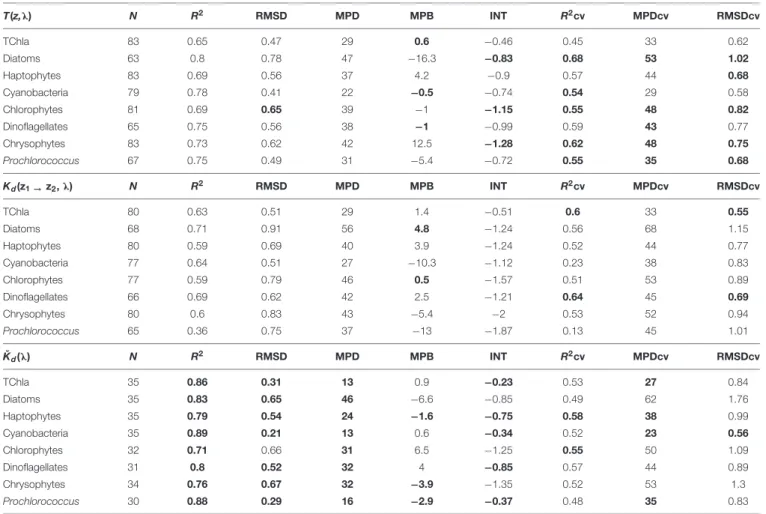
TABLE 3 |Full fit statistics of PS113 optical based TChla and PG Chla predictions against HPLC TChla and PG Chla data: number of the matchup points (N), determination coefficient (R2), intercept (INT), median percent bias (MPB), median percent difference (MPD), and root mean square difference (RMSD).
T(z,λ) N R2 RMSD MPD MPB INT R2cv MPDcv RMSDcv
TChla 83 0.65 0.47 29 0.6 −0.46 0.45 33 0.62
Diatoms 63 0.8 0.78 47 −16.3 −0.83 0.68 53 1.02
Haptophytes 83 0.69 0.56 37 4.2 −0.9 0.57 44 0.68
Cyanobacteria 79 0.78 0.41 22 −0.5 −0.74 0.54 29 0.58
Chlorophytes 81 0.69 0.65 39 −1 −1.15 0.55 48 0.82
Dinoflagellates 65 0.75 0.56 38 −1 −0.99 0.59 43 0.77
Chrysophytes 83 0.73 0.62 42 12.5 −1.28 0.62 48 0.75
Prochlorococcus 67 0.75 0.49 31 −5.4 −0.72 0.55 35 0.68
Kd(z1→z2,λ) N R2 RMSD MPD MPB INT R2cv MPDcv RMSDcv
TChla 80 0.63 0.51 29 1.4 −0.51 0.6 33 0.55
Diatoms 68 0.71 0.91 56 4.8 −1.24 0.56 68 1.15
Haptophytes 80 0.59 0.69 40 3.9 −1.24 0.52 44 0.77
Cyanobacteria 77 0.64 0.51 27 −10.3 −1.12 0.23 38 0.83
Chlorophytes 77 0.59 0.79 46 0.5 −1.57 0.51 53 0.89
Dinoflagellates 66 0.69 0.62 42 2.5 −1.21 0.64 45 0.69
Chrysophytes 80 0.6 0.83 43 −5.4 −2 0.53 52 0.94
Prochlorococcus 65 0.36 0.75 37 −13 −1.87 0.13 45 1.01
Kˇd(λ) N R2 RMSD MPD MPB INT R2cv MPDcv RMSDcv
TChla 35 0.86 0.31 13 0.9 −0.23 0.53 27 0.84
Diatoms 35 0.83 0.65 46 −6.6 −0.85 0.49 62 1.76
Haptophytes 35 0.79 0.54 24 −1.6 −0.75 0.58 38 0.99
Cyanobacteria 35 0.89 0.21 13 0.6 −0.34 0.52 23 0.56
Chlorophytes 32 0.71 0.66 31 6.5 −1.25 0.55 50 1.09
Dinoflagellates 31 0.8 0.52 32 4 −0.85 0.57 44 0.89
Chrysophytes 34 0.76 0.67 32 −3.9 −1.35 0.52 53 1.3
Prochlorococcus 30 0.88 0.29 16 −2.9 −0.37 0.48 35 0.83
Cross validation statistics (R2cv, MPDcv, and RMSDcv) are also presented. Models are differentiated among AOP input data set, T(z,λ), Kd(z1→z2,λ), and Kd(λ), as specified in Section “Hyperspectral AOP and Euphotic Depth Data” and “EOF Based Prediction of Phytoplankton Groups From Hyperspectral Underwater Data.” The correlations between predicted and HPLC PG Chla and TChla concentrations for these pigments were highly significant (p<0.0001). Bold highlights the best results among the three data sets.
Kd(z1→z2,λ) based model predictions. This is also supported by the recommendation of Lee et al. (2005) to rather choose a large depth interval for the calculation of Kd(z1 → z2, λ) in order to overcome the noise generated by wave introduced light fluctuations or high noise at low light levels. Therefore, given the fact that T(z, λ) data set provides overall the best cross validation statistics and that T(z, λ) based PG Chla and TChla data contain vertically resolved information reaching the deepest layers compared to those derived from the two other AOP variables, we selected this data set as being the most reliable data set. In the following we only use the predicted PG Chla and TChla data sets byT(z,λ) based models for comparison to similar data sets in other studies. Furtherone, we use this (now called ‘optical based prediction’) data set for demonstrating its applicability for obtaining highly resolved information on the phytoplankton abundance and composition in the water column of the Atlantic Ocean.
Our cross validation parameters obtained from the optical based PG and TChla predictions show comparable values (e.g., R2cv of 0.45–0.68, MPDcv of 29–53% and RMSDcv of 0.58–1.02)
to other studies that retrieve TChla and phytoplankton pigment concentrations from optical data sets. E.g.,Bracher et al. (2015), using in a similar region the same type of prediction models but based on field remote sensing reflectance data, obtained forR2cv, MPDcv and RMSDcv values ranging from 0.35 to 0.80, 28 to 43%, and 0.48 to 0.82.Chase et al. (2013)andLiu et al. (2019) derived phytoplankton pigments (different types of chlorophylls and the two major carotenoid groups) in the global and Arctic Ocean, respectively, by applying the Gaussian band method to hyperspectral IOP data from underway spectrophotometry; their validation results gave MPD values between 36–53% and 21–34%, respectively. Applying the matrix inversion technique inLiu et al.
(2019)to the same Arctic data set allowed for the quantification of more specific carotenoid pigments, however, with larger MDP values (37–65%).Sauzede et al. (2015)predicted fractions of PSC on TChla from fluorometric data using a neutral network based technique combined with the abundance based approach byUitz et al. (2006). Their validation results for the three PSC predictions against independent HPLC data gaveR2 values between 0.58–
0.72 and MPD values of 35–46%. Compared to Xi et al.
(2020) who employed the EOF based PG prediction models to satellite (multispectral) remote sensing reflectance data, our cross validation results based onT(z,λ) EOF models are for all PG groups and TChla better, except that theirR2cv value are slightly better for TChla and haptophytes (0.75 and 0.61, respectively).
In summary, our validation results indicate similar data quality as for the aforementioned methods predicting information on various phytoplankton pigment concentrations and fractions of PSC. We obtain even better quality for our models as compared to the PG Chla predictions byXi et al. (2020), which is especially the case for cyanobacteria andProchlorococcusChla. This may be caused by the higher regional consistency of our data sets, the hyperspectral data set giving more opportunities to find the best linear models for the predictions and that the HPLC data have been measured by only one laboratory which further reduces measurement uncertainty.
Phytoplankton Composition Along the Atlantic Transect
During our cruise in May–June 2018 transecting the Atlantic Ocean from the Patagonian Shelf to the English Channel, the surface water TChla from our HPLC data set ranged between 0.03 and 5.42 mg/m3. The HPLC TChla corresponded well to the satellite Chla derived from the Sentinel-3A OLCI within the same time frame (Figure 1A). To further characterize the phytoplankton composition and distribution along the cruise track, we discuss the results from our HPLC and optical based predictions PG data sets based on their clustering into the Longhurst provinces (Longhurst, 2007). In our study lowest (HPLC) TChla were 0.037 at the surface and 0.015 mg/m3 at depth which is above the values encountered in the clearest ocean waters (South Pacific Gyre) by Morel et al. (2007). The corresponding PG Chla can be smaller and since the detection limit of our HPLC system is 1µg/m3, we still kept all PG Chla above this value in the data set. However, following Xi et al.
(2020) we consider PG Chla below 0.005 mg/m3 to bear much larger uncertainty.
The hierarchical cluster analysis based on the HPLC PG data resulted in six clusters. The assignment of the HPLC surface stations into the clusters is depicted inFigure 1C. The location of the samples belonging to four of the six clusters reflected very well the geographic locations of specific Longhurst provinces from the Atlantic Ocean: Clusters I corresponded to the Southwest Atlantic Shelves (SWAS), Cluster III to the Canary Current Coast (CNRY), Cluster V to the Brazilian Current Coast (BRAZ), and Cluster VI to the Northeast Atlantic Shelves (NECS). Cluster IV stations fall into the North Atlantic Drift (NADR) and the Northern part of the North Atlantic Subtropical Gyre East (NASE-N). The remaining cluster contained all Atlantic Longhurst gyre regions crossed by our cruise, namely the South Atlantic Tropical Gyre (SATL), North Atlantic Tropical Gyre (NATR), the southern part of North Atlantic Subtropical Gyre East (here abbreviated as NASE), and the Western Tropical Atlantic (WTRA). By further testing within clusters II and IV the significance of the absolute values of the surface TChla, temperature and salinity, a clear
north-to-south structure could be distinguished and we finally could separate Cluster II into SATL, WTRA, NATR, and NASE, and Cluster IV into NASE-N and NADR stations.
As an outlier, one station within CNRY appeared within Cluster V (BRAZ).
Following the province assignment based on the HPLC derived surface PG data, our optical based predictions of PG Chla and TChla were classified into the aforementioned Longhurst provinces. PG data from HPLC and the optical based predictions show consistent patterns. This is also found for PG distributions at depths where they were observed (below this is detailed for the provinces SATL, WTRA, NATR, and CNRY). However, for a few of them (n= 7, all sampled on May 31, 2018) the upper part of each profile was following NATR PG composition, while the lower part was following CNRY PG composition, or vice versa.
This is consistent with the fact that in this region water from the open ocean North Atlantic intermixed on small horizontal and vertical scales with water from the Canary upwelling system (von Appen et al., 2020). Most optical stations (Table 4) were sampled in WTRA (>40%), closely followed by SATL (∼35%), and 10% were sampled each for the CNRY and NATR provinces.
Only very few optical profiles were available from NASE (n= 8) and only one each for SWAS and BRAZ. This diminishes the generality of the observed features in the vertical structure in these latter provinces. We obtained only surface HPLC based PG data and no optical measurements North of 36◦N (Table 4).
Therefore, NASE-N, NADR, and NECS can only be described briefly, while for the SATL, WTRA, CNRY, and NATR we can provide in-depth analysis.
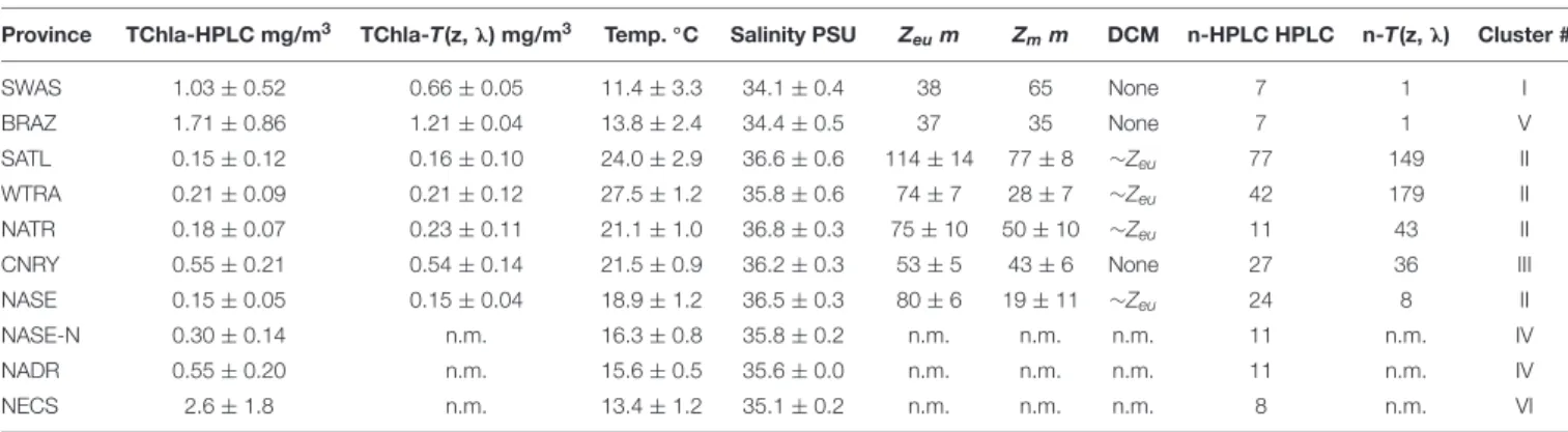
Mean and standard deviations (indicated as ±) for the fractions of PG Chla on TChla from the surface HPLC data are given inTable 5, and the surface HPLC-TChla, temperature and salinity measured from the thermosalinograph at all HPLC stations for each province are presented in Table 1. Figure 3 shows the depth resolved TChla along the whole cruise track from HPLC and optical based predictions. The latter match very well the values obtained from HPLC which is also supported by comparing the mean and standard deviation results in different Longhurst provinces for both data sets (Table 5).
The optical based TChla predictions always reach at least the Zeu (or even below), the depth where often the maximum biomass was obtained. Along our transect Zeu ranged from
∼25–120 m and Zm from 10 to 90 m. The surface PG Chla fraction predictions derived from the optical data set fall well within the standard deviation of fractions obtained from the HPLC data in all provinces (Figure 4). This is especially interesting as: (1) the optical data sampled two to three times more stations in the SATL, WTRA, CNRY, and NATR provinces (n = 149, n = 179, n = 43, and n = 36, respectively) than those by the HPLC data set (n= 77,n= 42, n = 13, and n = 13, respectively), and (2) the distribution of the sampled data was quite different for both data sets in these provinces. Mind that no robust predictions could be obtained for cryptophytes from the optical based data sets (see section “Prediction of Phytoplankton Groups From Hyperspectral Underwater Measurements”) while those were included in the calculation of the HPLC PG fractions. We
![FIGURE 2 | All spectra of the three types of AOP input data [upper panel: K d (z 1 → z 2 , λ), middle panel: T(z, λ), and lower panel: ˇK d (λ)] to EOF based PG and TChla prediction models](https://thumb-eu.123doks.com/thumbv2/1library_info/5209693.1668837/8.892.447.825.100.991/figure-spectra-types-input-middle-tchla-prediction-models.webp)
![TABLE 2 | Change in the Akaike information criterion for the robust PG Chla and TChla predictions by the EOF models based on three different types of AOP data sets [upper panel: T(z, λ), middle panel: K d (z 1 → z 2 , λ) and lower panel: K d (λ)], as speci](https://thumb-eu.123doks.com/thumbv2/1library_info/5209693.1668837/9.892.70.829.300.864/table-change-akaike-information-criterion-robust-predictions-different.webp)
![FIGURE 4 | Mean (bar) and standard deviation (line) of fraction of seven PG Chla on TChla as obtained from HPLC data (blue) and optical based [T(z,λ)] predictions (red) during PS113 for the five Longhurst provinces SATL, WTRA, NATR, CNRY, and NASE, as defi](https://thumb-eu.123doks.com/thumbv2/1library_info/5209693.1668837/13.892.70.829.94.458/figure-standard-deviation-fraction-obtained-predictions-longhurst-provinces.webp)
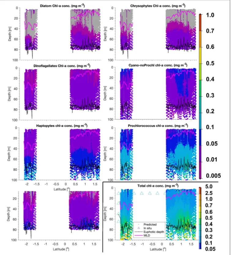
![FIGURE 5 | PG Chla and TChla from HPLC and optical based [T(z, λ )] predictions within the water column along a transect sampled with the Triaxus during PS113 on May 22, 2018 within the Longhurst province SATL](https://thumb-eu.123doks.com/thumbv2/1library_info/5209693.1668837/14.892.70.828.95.889/figure-optical-predictions-transect-sampled-triaxus-longhurst-province.webp)