Article
Retrieval of Phytoplankton Pigments from Underway Spectrophotometry in the Fram Strait
Yangyang Liu1,2,*, Emmanuel Boss3, Alison Chase3, Hongyan Xi1, Xiaodong Zhang4,5, Rüdiger Röttgers6, Yanqun Pan7,8and Astrid Bracher1,9
1 Alfred Wegener Institute Helmholtz Center for Polar and Marine Research, 27570 Bremerhaven, Germany;
hongyan.xi@awi.de (H.X.); astrid.bracher@awi.de (A.B.)
2 Faculty of Biology and Chemistry, University of Bremen, 28359 Bremen, Germany
3 School of Marine Sciences, University of Maine, Orono, ME 04469, USA; emmanuel.boss@maine.edu (E.B.);
alison.p.chase@maine.edu (A.C.)
4 Division of Marine Science, University of Southern Mississippi, Stennis Space Center, MS 39529, USA;
xiaodong.zhang@usm.edu
5 Department of Earth System Science and Policy, University of North Dakota, Grand Forks, ND 58202, USA
6 Helmholtz-Zentrum Geesthacht Center for Materials and Coastal Research, 21502 Geesthacht, Germany;
ruediger.roettgers@hzg.de
7 Department of Biology, Chemistry and Geography, Université du Québec à Rimouski, Rimouski, QC G5L 3A1, Canada; yanqun.pan@uqar.ca
8 State Key Laboratory of Estuarine and Coastal Research, East China Normal University, Shanghai 200241, China
9 Institute of Environmental Physics, University of Bremen, 28359 Bremen, Germany
* Correspondence: yangyang.liu@awi.de; Tel.: +49-471-4831-1785
Received: 21 December 2018; Accepted: 30 January 2019; Published: 6 February 2019 Abstract:Phytoplankton in the ocean are extremely diverse. The abundance of various intracellular pigments are often used to study phytoplankton physiology and ecology, and identify and quantify different phytoplankton groups. In this study, phytoplankton absorption spectra (aph(λ)) derived from underway flow-through AC-S measurements in the Fram Strait are combined with phytoplankton pigment measurements analyzed by high-performance liquid chromatography (HPLC) to evaluate the retrieval of various pigment concentrations at high spatial resolution.
The performances of two approaches, Gaussian decomposition and the matrix inversion technique are investigated and compared. Our study is the first to apply the matrix inversion technique to underway spectrophotometry data. We find that Gaussian decomposition provides good estimates (median absolute percentage error, MPE 21–34%) of total chlorophyll-a (TChl-a), total chlorophyll-b (TChl-b), the combination of chlorophyll-c1 and -c2 (Chl-c1/2), photoprotective (PPC) and photosynthetic carotenoids (PSC). This method outperformed one of the matrix inversion algorithms, i.e., singular value decomposition combined with non-negative least squares (SVD-NNLS), in retrieving TChl-b, Chl-c1/2, PSC, and PPC. However, SVD-NNLS enables robust retrievals of specific carotenoids (MPE 37–65%), i.e., fucoxanthin, diadinoxanthin and 190-hexanoyloxyfucoxanthin, which is currently not accomplished by Gaussian decomposition. More robust predictions are obtained using the Gaussian decomposition method when the observedaph(λ)is normalized by the package effect index at 675 nm. The latter is determined as a function of “packaged” aph(675) and TChl-a concentration, which shows potential for improving pigment retrieval accuracy by the combined use ofaph(λ)and TChl-a concentration data. To generate robust estimation statistics for the matrix inversion technique, we combine leave-one-out cross-validation with data perturbations. We find that both approaches provide useful information on pigment distributions, and hence, phytoplankton community composition indicators, at a spatial resolution much finer than that can be achieved with discrete samples.
Remote Sens.2019,11, 318; doi:10.3390/rs11030318 www.mdpi.com/journal/remotesensing
Keywords: phytoplankton pigments; phytoplankton absorption; underway AC-S flow-through system; Gaussian decomposition; matrix inversion; singular value decomposition; non-negative least squares
1. Introduction
Phytoplankton account for approximately half of global primary production via photosynthesis [1]
and form the base of the marine food web. Intracellular pigments of phytoplankton, composed of chlorophylls (a, b and c), carotenoids (carotenes and xanthophylls) and phycobiliproteins (phycoerythrin, phycocyanin and allophycocyanin) [2], play a vital role in photoprotection and the light-driven part of photosynthesis. Chlorophyll-b, -c and photosynthetic carotenoids (PSC), such as fucoxanthin (Fuco), act as antenna pigments that transfer the light energy to chlorophyll-a in the photosynthetic reaction centers of photosystems, assisting in light harvesting for photosynthesis.
In cyanobacteria, red algae, and cryptophytes, phycobiliproteins are the major light-harvesting pigments [3]. Chlorophyll-a is crucial in converting the received light energy to chemically bonded energy. The carotenoids not involved in photosynthesis are photoprotective (PPC). In particular, some xanthophylls such as violaxanthin (Viola), zeaxanthin (Zea), diadinoxanthin (Diadino) and diatoxanthin (Diato) are involved in the xanthophyll cycle, one of the most important photoprotective mechanisms that drives the non-radiative dissipation of the excess light energy to prevent photoinhibition [4,5]. Therefore, their relative abundance can be used as a tracer of photoacclimation processes [5].
In the context of global climate change, knowledge of the distributions of phytoplankton pigments is useful to understand the impacts of the changing environment on primary productivity [6], phytoplankton diversity and community composition through appropriate analysis, for example, CHEMTAX [7] and diagnostic pigment analysis [8]. In remote sensing applications, phytoplankton pigment databases have been extensively used to develop, validate, or refine bio-optical algorithms for estimating phytoplankton biomass (often estimated using total chlorophyll-a (TChl-a) concentration) and functional types (via diagnostic pigment analysis) based on both cell size (micro-, nano- and pico-phytoplankton) and biogeochemical functions (e.g., calcification, silicification, dimethyl sulphide production and nitrogen fixation) [9] and references therein. These data sets are mainly based on high-performance liquid chromatography (HPLC) analysis of discrete water samples. This technique enables the accurate quantification of 25–50 pigments in a single analysis [10]. However, it requires highly trained personnel, intensive labor and time, expensive and complex analysis, and is limited by the sampling frequency, spatial coverage and additional issues related to discrete sampling such as sample handling, storage and transportation. While HPLC pigment analysis remains indispensable, it is necessary to explore methods that enable easier access to pigment data at higher spatial-temporal resolution.
Because optical measurements are currently the only means of collecting synoptic scale information on upper ocean particles (e.g., operational open-ocean satellite ocean color provides data daily with pixel size down to 300 m by 300 m), attempts have been made to quantify the concentrations of various phytoplankton pigments from these measurements (e.g., absorption or reflectance spectra). Optical methods take advantage of the distinctive absorption characteristics of different pigments and various approaches are applied, such as the decomposition of spectra into Gaussian functions, e.g., [11], spectral reconstruction, e.g., [12], derivative analysis, e.g., [13], partial least squares regression, e.g., [14], multiple linear regression [15], reflectance band ratio, e.g., [16,17], principal component analysis, e.g., [18] and artificial neural networks [19,20].
The Gaussian decomposition method decomposes phytoplankton absorption spectra (aph(λ)) into Gaussian functions and correlates the amplitudes of the Gaussian functions with the concentrations of major pigment groups. The amplitude of each Gaussian function is assumed to represent the
magnitude of the absorption coefficient of a specific pigment or pigment group at the Gaussian peak wavelength, based on known pigment absorption properties determined in laboratory analyses.
This method simultaneously retrieves the concentrations of chlorophyll-a, chlorophyll-b, chlorophyll-c and carotenoids [11,21–23] or of chlorophyll-a and phycocyanin [24,25]. However, the retrieval accuracy is generally limited by the variations in pigment package effect of field samples. Nevertheless, the Gaussian absorption coefficients of specific pigment groups were recently incorporated into the reconstruction of hyper- and multi-spectral remote sensing reflectance, allowing the robust estimation of the concentrations of TChl-a, total chlorophyll-b (TChl-b), the combination of chlorophyll-c1 and -c2 (Chl-c1/2) and PPC globally [23] as well as of phycocyanin in cyanobacteria bloom waters [24,25]
from remote sensing reflectance data.
The spectral reconstruction method assumes thataph(λ)can be reconstructed from the linear combination of pigment-specific absorption coefficients multiplied by corresponding pigment concentrations [26]. Moisan et al. [27,28] applied matrix inversion analysis to the reconstruction model and successfully estimated the concentrations of a series of pigments directly from aph(λ). This technique involves a first inversion of the observed pigment concentrations that derives pigment-specific absorption spectra and a second inversion of these derived pigment-specific absorption spectra that solves for pigment concentrations. Four methods that solve least squares problems, i.e., singular value decomposition (SVD) [29], non-negative least squares (NNLS) [30]
and two nonlinear least squares minimization schemes based on the Levenberg–Marquardt algorithm [31,32] were compared for the two inversions. They found that when the first inversion was carried out with SVD and the second one with NNLS, the inverse modeling technique yielded the most accurate pigment estimates. However, the retrieval accuracy is affected by the level of correlation between pigment concentrations, the contribution of a specific pigment to the spectralaph(λ), pigment package effect, the missing absorption components by the pigments that exist in the samples but are not obtained by standard HPLC (e.g., mycosporine-like amino acids and phycobiliproteins) [27,28], and the number of spectral bands ofaph(λ)used in the inversion model [27,28,33]. Overall, the SVD-NNLS method achieved simultaneous statistically significant retrievals of TChl-a, total chlorophyll-c (TChl-c), β-carotene (β-Caro), Fuco, Viola, Diadino and peridinin (Peri) in U.S. east coast waters [27,28]. It was recently applied toaph(λ) modeled from MODIS-Aqua TChl-a data for northeastern U.S. waters, yielding maps of the concentrations of ten pigments [34]. Similar approaches were successful in infering phytoplankton size classes globally [35,36] and taxonomic groups in the Chukchi and Bering Seas [33]
from absorption data.
Derivative analysis of absorption spectra separates the secondary absorption peaks and shoulders contributed by phytoplankton pigments within the overlapping absorption regions [37].
Bidigare et al. [13] found that the fourth derivative maxima of particulate absorption spectra (ap(λ)) provided strong linear relationships with chlorophylls (a, b and c) concentrations in Sargasso Sea.
However, this method failed to estimate carotenoid concentrations because of the similarity of their spectral properties, the broad spectral absorption and relatively rounded absorption peaks that are less accessible to derivative analysis.
Principal component analysis (a.k.a. empirical orthogonal function analysis) derives several dominant modes (known as “principal components”) of the spectra that mainly account for the variability in spectral shape and relates them to pigment concentrations. Bracher et al. [18] performed this analysis on both hyperspectral and multispectral remote sensing reflectance data and retrieved the concentrations of TChl-a, monovinyl-chlorophyll-a, PPC, PSC, Chl-c1/2, 190-butanoyloxyfucoxanthin (But), 190-hexanoyloxyfucoxanthin (Hex), Zea, phycoerythrin and the sum ofα- andβ-Caro from the linear combinations of the principal components in the Atlantic Ocean. This method is, however, only applicable to the pigments that have been identified in most collocated samples. It failed to retrieve the pigments that are mostly absent or below detection limit. Similarly, Soja–Wo´zniak et al. [38] applied this analysis on both hyperspectral and multispectral remote sensing reflectance data and successfully retrieved TChl-a, phycocyanin and phycoerythrin in the Gulf of Gdansk.
An artificial neural network relates spectra to pigment data with a nonlinear model that self-adjusts the model parameters (i.e., weight matrix) for the best fit. Bricaud et al. [19] developed a multilayer perceptron using a global data set and obtained estimations of the concentrations of TChl-a, TChl-b, TChl-c, PSC and PPC, with TChl-a and TChl-b being the most accurate and poorest estimates, respectively. The main limitation of this method lies in the biological variability embedded in the training data set.
More recently, there has been an increased use of in situ hyperspectral optical sensors to obtain pigment data from continuous optical measurements, e.g., [22]. In-line and autonomous measurements by new miniature sensors deployed on various platforms (e.g., profiling floats, autonomous surface water vehicles) have substantially increased the sampling frequency and spatial coverage of measurements. The shipboard underway spectrophotometry considerably facilitates the acquisition ofap(λ) with unprecedented spatial resolution. It utilizes an AC-S hyperspectral spectrophotometer (or the 9-wavelength resolved AC-9) (Sea-Bird Scientific, Philomath, OR, USA) operated in flow-through mode and derives ap(λ) by differencing the bulk seawater absorption measurements from temporally adjacent 0.2-µm filtered water sample measurements, e.g., [22,39–48].
It has provided surface TChl-a data along cruise tracks via the empirical relationships between the spectrophotometry derived ap(λ) and HPLC measured TChl-a concentrations [39,40,45–48].
Furthermore, Gaussian decomposition has been performed by Chase et al. [22] to retrieve major pigment groups from a globally extensive underway AC-S derivedap(λ)data set. Here we use a data set obtained with a similar underway system to compare and contrast two different methods to obtain information on the underlying pigments.
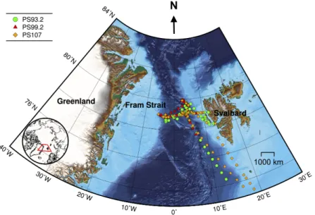
The Fram Strait, the region between Svalbard and Greenland, provides the only deep connection between the North Atlantic and Arctic Oceans (Figure1). It is of great importance to the climate in the Arctic region, as it accounts for 75% of the mass exchange and 90% of the heat exchange between the Arctic Ocean and the rest of the world’s ocean [49]. In recent decades, the Fram Strait has undergone a significant warming, high variability of Atlantic water inflow [50] and an overall increase of sea ice area export [51–55]. This impacts phytoplankton biomass, community composition and distribution by altering light and nutrient regimes. The seasonal cycle of phytoplankton biomass has been significantly enhanced in the shallow upper water layers since 2008 [56]. Phytoplankton distributions reflect the dominant local physical processes [56,57]. A significant increase in summertime chlorophyll-a concentration in the eastern Fram Strait was observed, whereas on the western side there were minor changes [56]. Furthermore, a shift of dominant phytoplankton assemblages from diatoms (mainlyThalassiosiraspp.,Chaetocerosspp. andFragilariopsisspp.) towards coccolithophores (mainlyEmiliania huxleyi) and more recently,Phaeocystisspp. (mainlyPhaeocystis pouchetii) and other small pico- and nanoflagellates during summer months was suggested [56,58,59], which can strongly affect the functioning and stability of marine food webs [60,61]. The studies of phytoplankton community composition in this region are mainly based on discrete water samples or moored sediment traps. Because of the inherent limitations of these methods, the observations are scarce.
Furthermore, it remains difficult to obtain information on phytoplankton community composition via satellite due to the poor spatial-temporal coverage of ocean color data in this region, e.g., [57]
and the lack of assessment of the applicability of satellite algorithms determining the phytoplankton community structure for this region. Additionally, algorithms applicable to other waters for quantifying phytoplankton community structure or pigment composition from in situ optical measurements have not been assessed yet in this region.
The Fram Strait cruises PS93.2, PS99.2 and PS107 on R/V Polarstern collected a comprehensive in situ bio-optical data set and offer a unique opportunity for bio-optical modeling. In particular, underway spectrophotometry was applied during all three cruises. To obtain the information of individual phytoplankton pigments or pigment groups (e.g., PSC and PPC) from underway spectrophotometry, here, we compare and optimize the performances of two pigment retrieval approaches, Gaussian decomposition [22] and the matrix inversion technique [27,28], find the potential
number and types of pigments that can be retrieved, and assess the applicability of the two approaches to the Fram Strait and its vicinity.
N
Figure 1.Cruise tracks for PS93.2 (July–August 2015), PS99.2 (June–July 2016) and PS107 (July–August 2017). Symbols denote locations where both AC-S and HPLC data were collected. Bathymetric grid data are extracted from the International Bathymetric Chart of the Arctic Ocean Version 3.0 [62].
Lambert azimuthal equal-area projection was used for mapping.
2. Data and Methods
2.1. Data Collection
Data were collected during three expeditions on R/V Polarstern: PS93.2 (July to August 2015), PS99.2 (June to July 2016) and PS107 (July to August 2017). These cruises have repeated survey design.
Sampling sites were located in the Fram Strait and its vicinity, ranging from approximately latitudes 72◦to 80◦N and longitudes 10◦W to 15◦E (Figure1).
The underwayap(λ)and discrete pigment concentration measurements of the surface water were collected for each expedition. The average velocity of the ship while moving is ~10 knots (5.1 m s−1).
Sampling methods and data analysis are detailed in Liu et al. [45]. Briefly, a 25-cm-pathlength AC-S spectrophotometer (spectral range: 400–740 nm, full width half maximum (FWHM): 10 nm, wavelength resolution: ~3.5 nm) was integrated into the shipboard flow-through system following the setup of Slade et al. [46]. Seawater was sampled at roughly 11 m below the sea surface from the ship’s keel using a membrane pump. The flow rate of seawater is 1–2 L min−1. Theap(λ)spectra were derived by subtracting the absorption coefficients of 0.2-µm filtered seawater from those of seawater materials measured by AC-S. Subsequently, they were corrected for temperature and salinity dependency of pure water absorption [63], scatter errors [64] and residual temperature effect [46]. Additionally, the effect of AC-S filter factors resulting in a smoothing of the measuredap(λ)spectra was corrected [22].
Discrete seawater samples were collected from the unfiltered AC-S outflow approximately every three hours. Seawater (1–3 L) was filtered with GF/F glass fiber filters (nominal pore size 0.7µm) for HPLC phytoplankton pigment analysis (see Table1for the names and abbreviations of the pigments and pigment groups used in this study). Pigments were grouped following Hooker et al. [65].
Divinyl-chlorophyll-a and divinyl-chlorophyll-b were not found in our data set. For convenience, in the following context, the term “pigment” stands for either a specific type of pigment or a pigment group such as PSC and PPC. In addition, the spectral absorption coefficient of non-algal particles (aN AP(λ)) in discrete water samples was measured for the determination of its spectral exponent. Seawater (0.2–1 L) was filtered to concentrate particulate materials on the GF/F filters. ap(λ)from discrete samples was
determined using Quantitative Filter Technique [66–68]. Measurements for samples from PS93.2 were carried out on a dual-beam UV/VIS spectrophotometer (Cary 4000, Varian Inc., Palo Alto, CA, USA) (spectral range: 300–850 nm, FWHM: 2 nm, wavelength resolution: 1 nm) equipped with a 150 mm integrating sphere following Simis et al. [69], whereas filters collected during PS99.2 and PS107 were measured using a small portable integrating cavity absorption meter (spectral range: 300–850 nm, FWHM: 2 nm, wavelength resolution: 0.3 nm) [70], as detailed in Liu et al. [45]. aN AP(λ)was then obtained by measuring the sample filters bleached with 10% NaClO solution [69] following the same procedure as ap(λ) measurements. aN AP(λ) was approximated using an exponentially decaying function [71,72]:
aN AP(λ) =aN AP(400)e−S(λ−400) (1) where S is the spectral exponent of aN AP(λ). Equation (1) was fit to aN AP(λ) for data between 380–620 nm excluding the 400–480 nm range (to eliminate residual chlorophyll-a absorption peak) using non-linear least squares method [72]. The median value ofSfor all three expeditions is 0.016 nm−1 (standard deviation with respect to the median value is 0.006 nm−1), which was subsequently used in the decomposition of the AC-S derivedap(λ)to obtainaph(λ)(see Section2.2.1).
AC-S derivedap(λ) were averaged within the period of ten minutes before and after HPLC sampling time and were matched with HPLC pigments data. aph(λ) (400–700 nm, wavelength resolution: ~3.5 nm) was obtained by numerical decomposition (see Section 2.2.1). In total, 298ap(λ)-pigments match-ups were obtained, which were subsequently used as the pigment retrieval data set. The link to the data used in this study is shared in the supplementary materials.
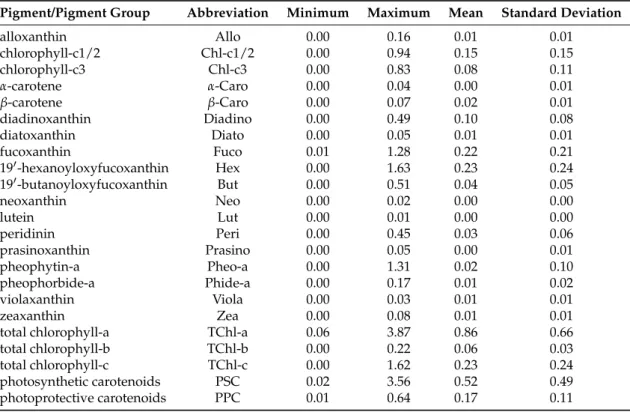
Table 1.Names and abbreviations of phytoplankton pigments and pigment groups analyzed in this study, and the minimum, maximum, mean and standard deviation of the pigment concentrations (mg m−3).
Pigment/Pigment Group Abbreviation Minimum Maximum Mean Standard Deviation
alloxanthin Allo 0.00 0.16 0.01 0.01
chlorophyll-c1/2 Chl-c1/2 0.00 0.94 0.15 0.15
chlorophyll-c3 Chl-c3 0.00 0.83 0.08 0.11
α-carotene α-Caro 0.00 0.04 0.00 0.01
β-carotene β-Caro 0.00 0.07 0.02 0.01
diadinoxanthin Diadino 0.00 0.49 0.10 0.08
diatoxanthin Diato 0.00 0.05 0.01 0.01
fucoxanthin Fuco 0.01 1.28 0.22 0.21
190-hexanoyloxyfucoxanthin Hex 0.00 1.63 0.23 0.24
190-butanoyloxyfucoxanthin But 0.00 0.51 0.04 0.05
neoxanthin Neo 0.00 0.02 0.00 0.00
lutein Lut 0.00 0.01 0.00 0.00
peridinin Peri 0.00 0.45 0.03 0.06
prasinoxanthin Prasino 0.00 0.05 0.00 0.01
pheophytin-a Pheo-a 0.00 1.31 0.02 0.10
pheophorbide-a Phide-a 0.00 0.17 0.01 0.02
violaxanthin Viola 0.00 0.03 0.01 0.01
zeaxanthin Zea 0.00 0.08 0.01 0.01
total chlorophyll-a TChl-a 0.06 3.87 0.86 0.66
total chlorophyll-b TChl-b 0.00 0.22 0.06 0.03
total chlorophyll-c TChl-c 0.00 1.62 0.23 0.24
photosynthetic carotenoids PSC 0.02 3.56 0.52 0.49
photoprotective carotenoids PPC 0.01 0.64 0.17 0.11
Note: TChl-a = monovinyl-chlorophyll-a + chlorophyllide-a; TChl-b = monovinyl-chlorophyll-b; TChl-c = Chl-c1/2 + Chl-c3; PSC = Fuco + But + Hex + Peri [65], PPC = Allo + Diadino + Diato + Zea +α- +β-Caro [65].
2.2. Retrieval of Phytoplankton Pigments
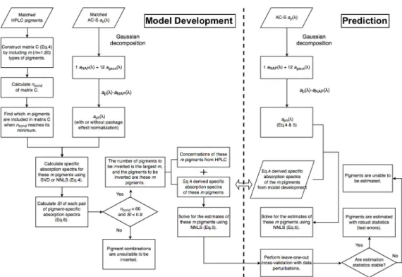
Figures2and3illustrate the steps of applying Gaussian decomposition and the matrix inversion technique, respectively, to retrieve phytoplankton pigment concentrations, which are described in detail
in the following subsections. The link to the codes for data processing is shared in the supplementary materials.
Figure 2.Schematic overview of the steps of applying Gaussian decomposition for phytoplankton pigment retrieval.
Figure 3.Schematic overview of the steps of applying the matrix inversion technique for phytoplankton pigment retrieval.
2.2.1. Gaussian Decomposition
Following Chase et al. [22], AC-S derivedap(λ)was decomposed to twelve Gaussian functions and one aN AP(λ) exponential function expressed by Equation (1) in the range of 400–700 nm.
Each Gaussian function represents the absorption by a certain phytoplankton pigment. The absorption by the water-soluble photosynthetic pigment phycoerythrin was also represented as a Gaussian function though its concentration could not be validated with HPLC. The peak location and width of each Gaussian function shown in Table2were defined with fixed values based on known pigment absorption shapes [73]. The decomposition is optimized by minimizing the cost function using a weighted least squares method [22]:
χ2=
700
∑
λ=400
[ap(λ)− 12∑
i=1
agaus,i(λ)−aN AP(λ)]2
σSD2 (λ) (2)
whereagaus,i(λ)denotes theith Gaussian function, andσSD(λ)is the standard deviation of the 20-min averaged matchedap(λ)spectra.
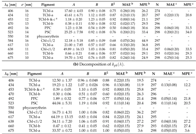
Table 2. The peak wavelengths (λ0) and widths (σ) of the Gaussian functions for phytoplankton pigments, the statistics for the power function regression ofagaus(λ0)-pigment pairs in the training set (regression coefficientsAandBof Equation (3) were calculated with 95% confidence bounds), and the statistics based on leave-one-out cross-validation. MAE is in mg m−3(values outside the parentheses were calculated with linear-scale values, while inside the parentheses with log10-scale values), MPE in
%, and N is the number of data points for the regressions.
(a)Decomposition ofaph(λ)
λ0[nm] σ[nm] Pigment A B R2 MAEb MPEb N MAEc MPEc
406 16 TChl-a 17.60±4.03 0.90±0.08 0.75 0.28(0.18) 26.2 274 - -
434 12 TChl-a 41.61±6.71 1.12±0.05 0.87 0.21(0.13) 20.7 297 0.22(0.13) 20.8
453 12 TChl-b & ca 1.18±0.20 1.23±0.05 0.92 0.00(0.14) 21.1 297 - -
470 13 TChl-b 0.38±0.11 0.50±0.08 0.52 0.02(0.17) 29.5 296 - -
492 16 PPC 1.23±0.38 0.54±0.09 0.50 0.06(0.18) 30.6 298 0.06(0.18) 31.5
523 14 PSC 25.25±7.58 0.92±0.08 0.76 0.20(0.21) 33.4 298 0.20(0.21) 34.0
550 14 phycoerythrin - - - - - - - -
584 16 Chl-c1/2 12.18±5.18 0.85±0.09 0.68 0.07(0.26) 44.9 297 - -
617 13 TChl-a 21.00±7.85 0.57±0.07 0.66 0.33(0.20) 36.8 295 - -
638 11 Chl-c1/2 49.89±16.13 1.03±0.06 0.81 0.05(0.20) 33.4 297 0.06(0.20) 33.5
660 11 TChl-b 0.66±0.21 0.44±0.06 0.57 0.02(0.16) 29.1 293 0.02(0.16) 29.3
675 10 TChl-a 19.70±3.92 0.76±0.05 0.82 0.24(0.14) 24.9 298 0.25(0.14) 25.3
(b)Decomposition of ˆaph(λ).
λ0[nm] Pigment A B R2 MAEb MPEb N MAEc MPEc
406 TChl-a 12.50±1.37 0.96±0.048 0.88 0.22(0.15) 19.5 274 - - 434 TChl-a 19.23±1.22 1.07±0.026 0.96 0.13(0.08) 11.9 297 0.13(0.08) 12.2 453 TChl-b & ca 0.39±0.05 1.10±0.05 0.92 0.00(0.15) 25.8 297 - -
470 TChl-b 0.30±0.06 0.51±0.07 0.60 0.02(0.15) 26.3 296 - -
492 PPC 1.89±0.32 0.77±0.06 0.77 0.05(0.14) 21.4 298 0.05(0.14) 21.8 523 PSC 44.04±5.31 1.19±0.04 0.92 0.11(0.14) 20.4 298 0.11(0.14) 20.5
550 phycoerythrin - - - - - - - -
584 Chl-c1/2 16.73±4.31 1.00±0.06 0.82 0.06(0.22) 36.2 297 - - 617 TChl-a 64.19±13.15 0.83±0.04 0.84 0.22(0.15) 24.1 295 - - 638 Chl-c1/2 34.11±7.20 1.06±0.05 0.91 0.04(0.17) 27.2 297 0.04(0.18) 27.2 660 TChl-b 0.47±0.12 0.41±0.05 0.62 0.02(0.15) 27.9 293 0.02(0.15) 27.4 675 TChl-a 33.57±0.72 1.00±0.01 1.00 0.05(0.03) 3.6 298 0.05(0.03) 3.6
a0.03(TChl-b) + 0.07(Chl-c1/2) [22,73];btraining errors;ctest errors based on cross-validation.
The amplitude ofaN AP(400)was derived by minimizing Equation (2) sample by sample and used to reconstructaN AP(λ) for each sample according to Equation (1). aph(λ) was obtained by
differencing ap(λ) and aN AP(λ). The amplitude of each Gaussian function agaus(λ0) [m−1] was derived by minimizing Equation (2) and related to the concentration of the corresponding pigment measured by HPLC (c[mg m−3]) by fitting the following equation using Bisquare robust non-linear least squares method (data pairs with eitheragaus(λ0)orcbeing 0 were excluded) (Table2):
c=A agaus(λ0)B (3)
For convenience, we denote the five pigments that can be retrieved using Gaussian decomposition (Table2), i.e., TChl-a, TChl-b, Chl-c1/2, PSC and PPC as “Gauss-5 pigments”.
2.2.2. Matrix Inversion Technique
Theaph(λ)spectra can be reconstructed as the linear combination of the absorption spectra of individual pigments that equal to the pigment-specific absorption coefficients (a∗j(λ)) multiplied by pigment concentrations (cj) [26], i.e.,aph(λ) =∑mj=1 cja∗j(λ). When there is more than one sample in the observed collocated pigment concentrations andaph(λ)data set, the reconstruction model can be written in matrix multiplication form as:
ci=1,j=1 · · · ci=1,j=m ... . .. ... ci=n,j=1 · · · ci=n,j=m
ea∗j=1(λ) ... ea∗j=m(λ)
=
aph,i=1(λ) ... aph,i=n(λ)
⇐⇒C·Ae =Aph (4)
wherecis the observed pigment concentration (e.g., from HPLC),ea∗(λ)is the derived pigment-specific absorption coefficient,nis the number of samples,iis the sample index,mis the number of pigments measured in each sample, and j is the pigment index. The c and aph(λ)are known (the former from HPLC and the latter from spectrophotometry) while ea∗(λ)is unknown. To solve for ea∗(λ), the elements of matrixA, the inverse of matrix C is computed. Once this is done, the derivede ea∗(λ)is used with the observedaph(λ)(lin Equation (5) is the number of wavelengths) to solve for the pigment concentrations (ecin Equation (5)). Likewise, the computation of the inverse of matrixA is necessary.e
ea∗j=1(λ1) · · · ea∗j=m(λ1) ... . .. ... ea∗j=1(λl) · · · ea∗j=m(λl)
eci=1,j=1...m
... cei=n,j=1...m
=
aph,i=1...n(λ1) ... aph,i=1...n(λl)
⇐⇒Ae·Ce=Aph (5)
Hence, this is a two step approach. First, where HPLC is available, Equation (4) is used to obtain the pigment-specific absorption spectra. Once those are available, Equation (5) is used to derive pigment concentrations directly fromaph(λ)(a step that does not require HPLC data). The SVD-NNLS approach proposed by Moisan et al. [27,28], i.e., solving Equation (4) with SVD least squares method on each wavelength and Equation (5) with NNLS method, was proved to give the best pigment estimates.
Singular Value Decomposition—Non-Negative Least Squares (SVD-NNLS)
The SVD-NNLS approach was adapted and tested using our data set. The matrix C in Equation (4) (the concentrations of the pigments listed in Table1) was inverted using SVD. The least-squares solution of the overdetermined Equation (4) (in this studyn>m) is derived byAe =C+·Aph, where C+ is the Moore-Penrose pseudoinverse of matrix C computed by SVD (MATLAB functionpinv).
A provides the specific absorption spectra of each pigment and is then used in Equation (5) to solve fore pigment concentrations via NNLS (MATLAB functionlsqnonneg), i.e., by inverting Equation (5) using least squares method with the constraintci,j ≥0.
To ensure robust solutions of the overdetermined systems, matrix C in Equation (4) and matrixAe in Equation (5) should be constructed to avoid ill-conditioning, requiring that the columns and rows of matrix C have sufficient linear independence, and that the shapes of any twoea∗(λ)be sufficiently
different from each other [36]. Here, we used the condition number (ncond) (MATLAB functioncond) as a diagnostic for the degree of the well-conditioning of matrix C (a matrix with a highncondis ill-conditioned, and vice versa). In addition, a similarity index (SIi,j) [74,75] was used to represent the similarity between the absolute values of two specific spectraaei∗
(λ)andaej∗
(λ)(denoted asea∗+(λ)).
TheSIi,jis a number ranging from 0 (no similarity) to 1 (perfect similarity).
SIi,j =1− 2
πarccos( aei
∗+(λ)·aej∗+(λ)
||aei∗(λ)|| ||aej∗(λ)||) (6) where||ea∗(λ)||is the norm of the vectorea∗(λ)(MATLAB functionnorm). To maximize the number of pigment types to be determined (m) while reducing the degree of the ill-conditioning, we tested all the possibilities of combining pigments composed of matrix C (number of combinations m!(20−m)!20! , 20 types of pigments measured in total) and examinedncondandSIi,jfor all cases. For example, when m= 20, matrix C includes all the pigments listed in Table1excluding TChl-c, PSC and PPC (denoted as “Fram-20 pigments”) in 298 samples . When 1≤m< 20, matrix C includes the concentrations ofm types of pigments and a summed contribution of other pigments included in the Fram-20 pigments.
mwas then determined as the biggest number withncondsmaller than 60 andSIi,jsmaller than 0.9.
For convenience, we denote the retrieval of thesempigments using SVD-NNLS as SVD-NNLS-m.
To compare with the results from Gaussian decomposition, the SVD-NNLS method was also applied to only retrieve Gauss-5 pigments (denoted as SVD-NNLS-50), i.e., matrix C in Equation (4) only includes the concentrations of these five pigments and a summed contribution of other pigments.
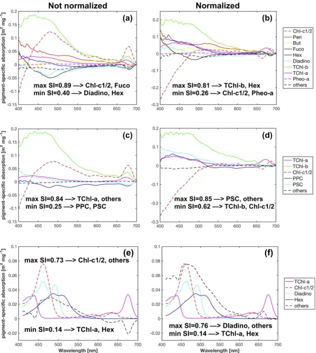
The SVD derived specific absorption spectra are purely mathematical solutions. Therefore, they are expected to be different from those obtained through laboratory measurements performed on the extracted individual pigments in solution (a∗(λ)) [27]. For comparison, we tested the validity of NNLS in estimating pigment concentrations usinga∗(λ)from Bricaud et al. [73] in Equation (5). In this case,a∗(λ)is available for 12 types of pigments (Divinyl-chlorophyll-a and divinyl-chlorophyll-b not considered), i.e., TChl-a, TChl-b, alloxanthin (Allo), But, Chl-c1/2, Diadino, Fuco, Hex, Peri, Zea, α- andβ-Caro (denoted as “Bricaud-12 pigments”). The same criteria ofncond andSIi,j were used for all pigment combinations (number of combinations m!(12−m)!12! ). For each combination, thea∗(λ) for the pigments which are missing in the Fram-20 pigments was solved using SVD (Equation (4), a∗j(λ)replacesea∗j(λ)). We denote this case as Bricaud-SVD-NNLS, and the retrieval ofmpigments as Bricaud-SVD-NNLS-m.
Non-Negative Least Squares—Non-Negative Least Squares (NNLS-NNLS)
Though SVD provides a powerful tool for matrix inversion, one concern is that the SVD derived specific absorption spectra can be negative, which are physically unsound and not intuitively understood. To cope with this issue, NNLS was used twice (denoted as NNLS-NNLS), i.e., to invert Equation (4) to solve for the non-negetive matrixA, as well as to invert Equation (5) to derive thee non-negative matrixC. Similarly, NNLS-NNLS-5e 0was tested for comparison with the results from Gaussian decomposition and SVD-NNLS-50. Bricaud-NNLS-NNLS were also tested using the same way as Bricaud-SVD-NNLS with the exception that thea∗(λ)for the missing pigments was solved using NNLS. The NNLS-NNLS approach was also performed by Moisan et al. [27,28]. The pigment estimation results from NNLS-NNLS are provided in AppendixA.
Sensitivity Analysis
The solution of matrix inversion can be sensitive to input errors depending on the degree of well-conditioning of the input matrices, which can affect the pigment estimation accuracy. To ensure the stability of the matrix inversion model and obtain reliable pigment estimation statistics, perturbations were introduced to the input data for 300 iterations, and the related parameters, i.e.,ncond,SI,ea∗(λ) and cross-validation statistics (see Section2.2.4) were calculated as the median values of the 300 sets.
Assuming an uncertainty of 15% for HPLC pigment data, matrix C was perturbed with random values within±15% of the measurements. Matrix Aphwas also perturbed by adding the random values within±σSD(λ)(see Equation (2)) to the measurements. The results for three cases, i.e., with perturbed C, with perturbed Aphand with both matrices perturbed were considered for both SVD-NNLS and NNLS-NNLS.
2.2.3. Normalization ofaph(λ)by Pigment Package Effect
The pigment package effect indexQ∗a(λ)can be calculated as the ratio of the measuredaph(λ) to the absorption coefficient of the same pigments which would be dispersed into solution [73,76].
To partially account for the package effect, Moisan et al. [27,28,34] normalized the measuredaph(λ) by dividing it withQ∗a(675) and found improved capability of the matrix inversion technique in retrieving pigment concentrations. To test the performances of both Gaussian decomposition and the matrix inversion technique with the normalization strategy,Q∗a(675)was calculated, andaph(λ)was normalized following
ˆ
aph(λ) =aph(λ) 0.033cTChl-a
aph(675) (7)
where cTChl-a is TChl-a concentration (in mg m−3), 0.033 (in m2 mg−1) is the “unpackaged”
Chl-a-specific absorption coefficient at 675 nm measured by Bricaud et al. [73], and the fraction is the inverse ofQ∗a(675). Note that chlorophyll-a, divinyl-chlorophyll-a, chlorophyll-b, divinyl-chlorophyll-b and Chl-c1/2 absorb light at 675 nm, e.g., [12,73]. For simplicity, we assume thatQ∗a(675)is only contributed by TChl-a, not only because TChl-a contributes most toaph(675), but also due to the weaker dependence on pigment data forQ∗a(675)calculation. In theory,Q∗a(675)ranges from 0 (fully
“packed”) to 1 (“unpackaged”). Due to uncertainties, samples with calculatedQ∗a(675)greater than 1 are unavoidable in practise and included in the calculation of ˆaph(λ).
The ˆaph(λ)was subsequently used to retrieve pigment concentrations via Gaussian decomposition, SVD-NNLS and NNLS-NNLS methods. Results were compared with those usingaph(λ). To avoid confusion, in the following context, unless otherwise stated, the results are based onaph(λ).
2.2.4. Statistics
For the development of pigment retrieval models, all the match-up points were used as training data, allowing the models to best account for the biological variations in the data set. Statistics for applying the model to the training data include the slope and the intercept of Model-1 Bisquare robust linear regression, the determination coefficient (R2), the mean absolute error (MAE) and the median absolute percentage error (MPE). The equations for the statistical metrics are given below:
MAE= 1 n
∑
n i=1|eci,j−ci,j| (8)
MPE=median o f |eci,j−ci,j|
ci,j ×100% (9)
wherenis the number of samples,ci,jis the concentration of thejth pigment in theith sample measured by HPLC, andeci,jis the estimated pigment concentration. Considering phytoplankton pigments are approximately log-normally distributed in the ocean, the slope, intercept andR2were computed in log10 space. Additionally, MAE is also calculated using log10(ci,j). To avoid confusion, in the following context, unless otherwise stated, MAE values are calculated usingci,j.
For model evaluation, leave-one-out cross-validation was performed (MATLAB function crossvalind) to estimate likely performance of each model on out-of-sample data. The pigment retrieval data set withNdata points was split into two partitions: one partition is the testing set with one data point, and the other partition is the training set with the union of the other data points. Statistics were
iteratively calculatedNtimes, using a different data point as the testing set each time. The model prediction errors for out-of-sample data were defined as the average values of the statistics (mean value for MAE and median value for MPE, respectively) for theNsets. Cross-validation is an effective way of estimating model test errors when the number of data available is relatively small [18,77]. Compared to the random train/test split method andk-fold cross-validation, leave-one-out cross-validation has the advantage that the training set highly resembles the whole data set (the former has only one data point less than the latter), thus avoids the bias introduced to the estimation of the test errors due to less training data than data available.
For clarity, statistics (errors) obtained from running the trained model back on the training data are denoted as “training statistics (errors)”, while those obtained when applying the trained model to the test data are called “test (or estimation or prediction) statistics (errors)”.
3. Results
3.1. Characteristics of the Pigment Retrieval Data Set
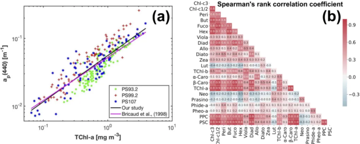
The magnitudes ofap(440)andap(675)vary in the range of 0.007–0.258 m−1(median: 0.043 m−1) and 0.001–0.086 m−1(median: 0.013 m−1), respectively. Overall,ap(440)varies as a power function of TChl-a concentration (Bisquare robust regression): ap(440) = 0.056 (cTChl-a)0.682 (R2= 0.82, MAE = 0.01 m−1). This relationship is close to the one derived by Bricaud et al. [71] for Case-1 waters (Figure4a). TChl-a can also be related toaph(675)via the cruise-specific power functions (Bisquare robust regression):cTChl-a =56.46aph(675)0.984(R2= 0.96, MAE = 0.12 mg m−3) (PS93.2), cTChl-a=26.3aph(675)0.935(R2= 0.96, MAE = 0.14 mg m−3) (PS99.2), andcTChl-a=119.1aph(675)1.217 (R2= 0.95, MAE = 0.17 mg m−3) (PS107).
The composition and data range of pigments (minimum, maximum, mean and standard deviation) are shown in Table1. TChl-a concentration spans the range 0.06–3.87 mg m−3. Only TChl-a, TChl-c, Fuco, Hex and PSC have a mean concentration greater than 0.2 mg m−3. Other than that, the pigments with mean concentrations greater than 0.05 mg m−3are Chl-c1/2, Diadino, TChl-b, and PPC. Large standard deviations were observed within individual pigments, and the ratios of standard deviation to mean value are in the range of 0.58–4.35. The correlation between the concentrations of phytoplankton pigments was represented by the Spearman0s rank correlation coefficient (Spearman’sρ) (Figure4b).
High level of the correlation (e.g., Spearman’sρ > 0.7 or <−0.7) is a concern as it can cause the ill-conditioning of Equation (4), influencing the accuracy of pigment estimation using the matrix inversion technique.
Figure 4. (a) Variations of the AC-S derived ap(440)as a power function of TChl-a concentration;
(b) the Spearman0s rank correlation coefficients between the concentrations of phytoplankton pigments in our data set (linear color bar scale).
3.2. Gaussian Decomposition
Strong correlations were found between the Gaussian function amplitudes and the corresponding pigment concentrations (R2 > 0.5) (Table2(a)). Among all the Gaussian functions representing TChl-a absorption, the amplitude at 434 nm has the strongest relationship to TChl-a concentration (R2= 0.87, MAE = 0.21 mg m−3), closely followed by that at 675 nm. agaus(638) is much better correlated with Chl-c1/2 thanagaus(584), whileagaus(660)provides slightly better correlation with TChl-b thanagaus(470). That theR2for TChl-b and PPC is smaller than 0.6 is likely due to the reduced dynamic range of TChl-b and PPC compared to TChl-a, Chl-c1/2 and PSC (Table1). Considering the relationships for PSC and PPC as well as the strongest correlations for TChl-a, TChl-b and Chl-c1/2, the MPE ranges from 20.7% to 33.4%. The training errors for the five pigments increase in the order of:
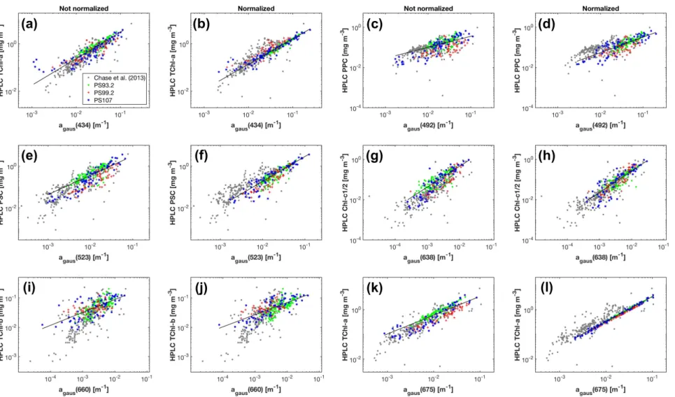
TChl-a, TChl-b, PPC, Chl-c1/2 and PSC. The strongest correlations for all five pigments are shown in Figure5a,c,e,g,i. For comparison, TChl-a is also plotted againstagaus(675)in Figure5k.
As a result of the above,agaus(434),agaus(660),agaus(638),agaus(523)andagaus(492)were used to predict the concentrations of TChl-a, TChl-b, Chl-c1/2, PSC and PPC, respectively. Statistics based on leave-one-out cross-validation (Table2(a)) show that overall, all five pigments were reasonably well retrieved (MPE 20.8–34.0%). TChl-a and TChl-b have the least and the second least prediction errors, respectively, while PSC is most poorly estimated.
When using ˆaph(λ), the performance of the Gaussian decomposition significantly improved.
Strong contrast was observed in the relationships between the Gaussian function amplitudes and pigment concentrations before and after applying the package effect normalization according to Equation (7) (Figure5, Table2(b)). All statistical parameters for the eleven relationships between Gaussian absorption and pigment concentrations are improved (Table2(b)). TheR2foragaus(434)to TChl-a correlation is 0.96 (0.87 before the normalization) and the regression coefficientB(Equation (3)) is close to one. Similarly, the R2 for agaus(638) to Chl-c1/2 correlation is 0.91 (0.81 before the normalization) and the regression coefficientB(Equation (3)) is also close to one. The relationships for PSC and PPC also improved in terms of increasedR2and decreased MAE and MPE for both pigments, and of a much closer shift ofB(Equation (3)) to one for PPC. In contrast, the relationship for TChl-b is least affected by the package effect normalization ofaph(λ), with still increasedR2, but only slightly decreased MAE and MPE, and a relatively large deviation ofB(Equation (3)) to the unity (0.35–0.60 for both 470 nm and 660 nm regardless of the normalization). Cross-validation results (Table2(b)) further confirm the improved performance of Gaussian decompostion in estimating TChl-b, Chlc1/2, PPC and PSC after taking the package effect into account (MPE 29.3–34.0% before the normalization and 20.5–27.4% afterwards). The pigment with the lowest estimated accuracy is now Chl-c1/2, but still with an improved accuracy following normalization. Similarly, TChl-b retrievals have slightly reduced MAE and MPE than those before the normalization.
Figure 5.Concentrations of phytoplankton pigments measured by HPLC versus the magnitudes of the corresponding Gaussian functions obtained from the Gaussian decomposition of bothaph(λ)(a,c,e,g,i) and ˆaph(λ)(b,d,f,h,j,l). The results of Chase et al. [22] are based onaph(λ).
3.3. Matrix Inversion Technique
3.3.1. The Number of Pigment Types to Be Estimated
To apply the matrix inversion technique to estimate phytoplankton pigments, a key issue is to determine the number of pigmentsmincluded in matrix C in Equation (4). Table3summarizes the final selections ofmthat fulfilled the criteria mentioned in Section2.2.2and the correspondingncond
andSIfor all cases of the matrix inversion technique. Thencondand maximum values ofSIdid not significantly change after data perturbations were introduced, regardless of the application of the package effect normalization.
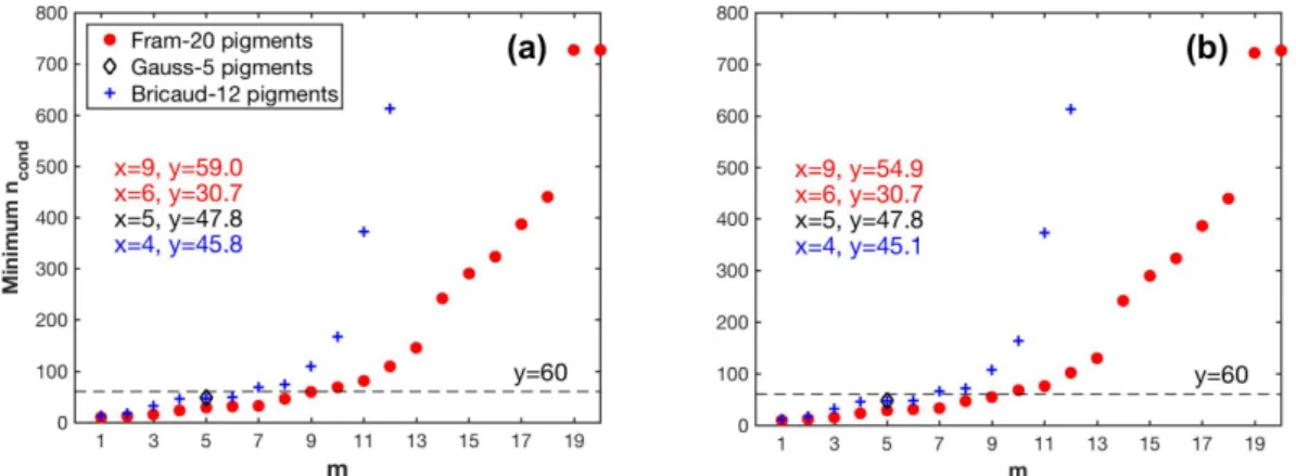
As shown in Figure6, the minimum values ofncondfor all pigment combinations increase with increasingm, indicating that the larger the number of pigment types to be estimated, the more sensitive the matrix inversion is to input errors. The largest value ofmis nine and six for all combinations of Fram-20 and Bricaud-12 pigments, respectively, with the minimum value ofncondsmaller than the threshold 60. When composed of Gauss-5 pigments, matrix C has ancondof 47.8.
Based on the results fulfilling thencondcriterion, whenea∗(λ)is derived by SVD, theSIcriterion allowedmto reach nine out of the Fram-20 pigments, and was satisfied by the Gauss-5 pigments.
However,mfor the NNLS-NNLS method decreased to six for of the Fram-20 pigments when package effect normalization was not performed, because the NNLS algorithm set some of the derivedea∗(λ) in the pigment combinations (m> 6) to zero to avoid negative values [30]. When the package effect normalization was applied, the number of pigment combinations valid forSIcalculation increased to nine, possibly because this normalization increases the inner differences of the set of the derivedea∗(λ). However, the maximumSI value exceeded 0.9 for Gauss-5 pigments. Therefore, NNLS-NNLS-50 method based on ˆaph(λ)was not considered in the estimation of pigments. As for the Bricaud-12 pigments, the choice of SVD and NNLS influences the derived specific absorption of the missing pigments, as indicated by the differentSIvalues. In this case,mreaches four. The specific pigments to be inverted for all cases are shown in Tables4and5and TableA1.
Figure 6.Variations in the minimum values of the condition number (ncond) of matrix C in Equation (4) with different pigment combination (mpigment types to be estimated): (a) pigment data unperturbed;
(b) pigment data perturbed.
Table 3. Them types of pigments to be estimated using the matrix inversion technique and the correspondingncondand maximumSIvalues.
(a)Pigment data perturbed
Method Pigments aph(λ)Based aˆph(λ)Based ncond MaximumSI m ncond MaximumSI m
SVD-NNLS Fram-20 54.9 0.86 9 54.9 0.85 9
NNLS-NNLS Fram-20 30.7 0.79 6 54.9 0.86 9
SVD-NNLS-50 Gauss-5 47.8 0.81 5 47.8 0.84 5
NNLS-NNLS-50 Gauss-5 47.8 0.79 5 47.8 - 5
Bricaud-SVD-NNLS Bricaud-12 45.1 0.72 4 45.1 0.76 4
Bricaud-NNLS-NNLS Bricaud-12 45.1 0.83 4 45.1 0.76 4
(b)aph(λ)data perturbed
Method Pigments aph(λ)Based aˆph(λ)Based ncond MaximumSI m ncond MaximumSI m
SVD-NNLS Fram-20 59.0 0.86 9 59.0 0.81 9
NNLS-NNLS Fram-20 30.7 0.75 6 59.0 0.85 9
SVD-NNLS-50 Gauss-5 47.8 0.74 5 47.8 0.82 5
NNLS-NNLS-50 Gauss-5 47.8 0.78 5 47.8 - 5
Bricaud-SVD-NNLS Bricaud-12 45.8 0.72 4 45.8 0.76 4
Bricaud-NNLS-NNLS Bricaud-12 45.8 0.83 4 45.8 0.76 4
(c)Both pigment andaph(λ)data perturbed
Method Pigments aph(λ)Based aˆph(λ)Based ncond MaximumSI m ncond MaximumSI m
SVD-NNLS Fram-20 54.9 0.84 9 54.9 0.81 9
NNLS-NNLS Fram-20 30.7 0.81 6 54.9 0.86 9
SVD-NNLS-50 Gauss-5 47.8 0.79 5 47.8 0.82 5
NNLS-NNLS-50 Gauss-5 47.8 0.80 5 47.8 - 5
Bricaud-SVD-NNLS Bricaud-12 45.1 0.72 4 45.1 0.76 4
Bricaud-NNLS-NNLS Bricaud-12 45.1 0.83 4 45.1 0.76 4
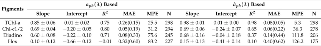
Table 4. Statistics for the Model-1 linear regressions between SVD-NNLS retrieved and measured pigment concentrations (regression coefficients were calculated with 95% confidence bounds). MAE is in mg m−3(values outside the parentheses were calculated with linear-scale values, while inside the parentheses with log10-scale values), MPE in %, and N is the number of data points for the regressions.
Unperturbed training data set was used.
(a)SVD-NNLS-9
Pigments aph(λ)Based aˆph(λ)Based
Slope Intercept R2 MAE MPE N Slope Intercept R2 MAE MPE N
TChl-a 0.97±0.04 0.00±0.01 0.92 0.15(0.10) 12.8 295 1.00±0.00 −0.00±0.00 1.00 0.01(0.01) 0.74 298 TChl-b 0.31±0.15 −0.81±0.20 0.31 0.04(0.32) 58.3 268 0.41±0.15 −0.70±0.20 0.25 0.04(0.30) 52.6 269 Chl-c1/2 0.65±0.06 −0.21±0.06 0.72 0.06(0.25) 42.6 286 0.60±0.06 −0.27±0.07 0.63 0.06(0.26) 37.1 275 But 0.43±0.10 −0.53±0.17 0.38 0.04(0.43) 100.0 209 0.54±0.08 −0.45±0.14 0.62 0.03(0.35) 62.6 206 Diadino 0.39±0.07 −0.45±0.08 0.40 0.06(0.30) 57.8 283 0.38±0.08 −0.52±0.09 0.46 0.06(0.30) 49.2 284 Fuco 0.84±0.06 −0.03±0.06 0.82 0.08(0.23) 33.7 276 0.85±0.06 −0.07±0.06 0.79 0.07(0.22) 31.6 286 Hex 0.62±0.05 −0.16±0.05 0.69 0.09(0.24) 37.3 266 0.72±0.04 −0.13±0.04 0.83 0.07(0.20) 32.0 270 Peri 0.74±0.15 −0.30±0.23 0.54 0.04(0.36) 57.5 134 0.67±0.17 −0.37±0.26 0.43 0.05(0.40) 66.6 128 Pheo-a 0.06±0.87 −0.31±0.65 -0.16 0.59(0.53) 166.0 22 −0.04±1.02 −0.39±0.77 −0.34 0.64(0.58) 132.0 22