High-Resolution Snow Depth on Arctic Sea Ice From Low-Altitude Airborne Microwave Radar Data

(1)

This article has been accepted for inclusion in a future issue of this journal. Content is final as presented, with the exception of pagination.

IEEE TRANSACTIONS ON GEOSCIENCE AND REMOTE SENSING 1

High-Resolution Snow Depth on Arctic Sea Ice From Low-Altitude Airborne Microwave Radar Data

Arttu Jutila , Joshua King , John Paden , Senior Member, IEEE, Robert Ricker , Stefan Hendricks , Chris Polashenski , Veit Helm , Tobias Binder , and Christian Haas

Abstract— We present new high-resolution snow depth data on Arctic sea ice derived from airborne microwave radar mea- surements from the IceBird campaigns of the Alfred Wegener Institute (AWI) together with a new retrieval method using signal peakiness based on an intercomparison exercise of colocated data at different altitudes. We aim to demonstrate the capabilities and potential improvements of radar data, which were acquired at a lower altitude (200 ft) and slower speed (110 kn) and had a smaller radar footprint size (2-m diameter) than previous airborne snow radar data. So far, AWI Snow Radar data have been derived using a 2–18-GHz ultrawideband frequency- modulated continuous-wave (FMCW) radar in 2017–2019. Our results show that our method in combination with thorough calibration through coherent noise removal and system response deconvolution significantly improves the quality of the radar- derived snow depth data. The validation against a 2-D grid of in situ snow depth measurements on level landfast first-

Manuscript received October 1, 2020; revised December 24, 2020 and February 19, 2021; accepted February 24, 2021. The authors acknowledge support by the Open Access Publication Funds of Alfred-Wegener-Institut Helmholtz-Zentrum für Polar- und Meeresforschung. The CReSIS toolbox used in this work was generated with support from the University of Kansas, NASA Operation IceBridge grant NNX16AH54G, and NSF grants ACI-1443054, OPP-1739003, and IIS-1838230. Development and aircraft integration of the AWI Snow Radar system was made possible with support from Bundesministeriums für Bildung und Forschung (BMBF) grant 03F0700A. The work of Arttu Jutila was supported by the Helmholtz Graduate School for Polar and Marine Research (POLMAR) Short-Term Research Grant for visiting the ECCC Climate Processes Section in Toronto, ON, Canada.

The work of Chris Polashenski was supported by the U.S. National Science Foundation under Grant ARC-1603361.(Corresponding author: Arttu Jutila.) Arttu Jutila, Robert Ricker, Stefan Hendricks, and Christian Haas are with the Sea Ice Physics Section, Alfred-Wegener-Institut Helmholtz-Zentrum für Polar-und Meeresforschung (AWI), 27570 Bremerhaven, Germany (e-mail:

arttu.jutila@awi.de; robert.ricker@awi.de; stefan.hendricks@awi.de; christian.

haas@awi.de).

Joshua King is with the Climate Research Division, Environment and Climate Change Canada (ECCC), Toronto, ON M3H 5T4, Canada (e-mail:

joshua.king@canada.ca).

John Paden is with the Center for Remote Sensing of Ice Sheets (CReSIS), University of Kansas, Lawrence, KS 66045 USA (e-mail: paden@ku.edu).

Chris Polashenski is with the U.S. Army Corps of Engineers, Cold Regions Research and Engineering Laboratory (USACE-CRREL) Alaska Projects Office, Fort Wainwright, AK 99703 USA, and also with the Thayer School of Engineering, Dartmouth College, Hanover, NH 03755 USA (e-mail:

chris.polashenski@gmail.com).

Veit Helm is with the Glaciology Section, Alfred-Wegener-Institut Helmholtz-Zentrum für Polar- und Meeresforschung (AWI), 27570 Bremerhaven, Germany (e-mail: veit.helm@awi.de).

Tobias Binder was with the Glaciology Section, Alfred-Wegener-Institut Helmholtz-Zentrum für Polar- und Meeresforschung (AWI), 27570 Bremer- haven, Germany. He is now with Ibeo Automotive Systems GmbH, 22143 Hamburg, Germany (e-mail: tobias.binder@ibeo-as.com).

Color versions of one or more figures in this article are available at https://doi.org/10.1109/TGRS.2021.3063756.

Digital Object Identifier 10.1109/TGRS.2021.3063756

year ice indicates a mean bias of only 0.86 cm between radar and ground truth. Comparison between the radar-derived snow depth estimates from different altitudes shows good consistency.

We conclude that the AWI Snow Radar aboard the IceBird campaigns is able to measure the snow depth on Arctic sea ice accurately at higher spatial resolution than but consistent with the existing airborne snow radar data of NASA Operation IceBridge. Together with the simultaneous measurements of the total ice thickness and surface freeboard, the IceBird campaign data will be able to describe the whole sea-ice column on regional scales.

Index Terms— Airborne, microwave, radar, sea ice, snow.

I. INTRODUCTION

A

KEY FACTOR contributing to our current limited knowledge of snow on sea ice and its importance to polar climate is the lack of representative snow observations. As a layer separating dynamic sea ice and atmosphere, snow exhibits heterogeneity that evolves over time and varies in space through different scales. Characterizing the spatial and temporal variability of snow with point scale in situmeasurements in a harsh and dynamic sea-ice environment is logistically challenging [1]. Satellite remote sensing of snow depth offers a practical solution through two main approaches. Brightness temperatures from multifrequency passive microwave sensors [2], their gradient ratios [3]–[5], or combined with emission modeling [6] are found to correlate with snow depth. A dual- altimetry method uses radars of two different frequencies, of which one is assumed to penetrate the snow, while the other is used to retrieve the air–snow interface [7], [8]. Recently, Kwok and Markus [9] and Kwoket al.[10] presented a combination of radar and laser satellite altimeters to estimate snow depth. However, data from satellite systems are constrained by spatiotemporal coverage, spatial resolution and differences in footprint size, surface roughness, ice type, and availability of ground measurements for validation [1]. Airborne observations are often used to validate satellite measurements even though they share many of the same constraints. In addition, measurements from different platforms need intercomparison to minimize uncertainty if the blended analysis is required.

Snow on Arctic sea ice modulates the thickness of the underlying ice [11]: in winter, it retards ice growth due to its low thermal conductivity [12]; in spring and summer, the high albedo of snow delays surface melt and melt pond formation [13], [14]. Moreover, snow contributes significantly to sea-ice mass balance through snow–ice formation [15]–[17].

This work is licensed under a Creative Commons Attribution 4.0 License. For more information, see https://creativecommons.org/licenses/by/4.0/

(2)

In addition, snow loading is a critical parameter to estimate sea-ice thickness from satellite radar and laser altimeter measurements through the assumption of hydrostatic equilibrium [18], [19]. Studies have shown that the widely used snow depth climatology in [20], derived from in situ measurements on multiyear ice (MYI) during 1951–1991, requires adjustments for applications on Arctic sea ice due to large interannual variability and basin-wide thinner, younger ice [1], [21]–[23].

Despite the high importance of snow on sea ice to polar climate, “snow depth on sea ice is essentially unmeasured” as expressed by the Intergovernmental Panel on Climate Change (IPCC) Special Report on the Ocean and Cryosphere in a Changing Climate (SROCC) [24].

Frequency-modulated continuous-wave (FMCW) radars have been used for snow research for more than 40 years and on airborne platforms since the 2000s [25]. Since 2009, NASA’s Operation IceBridge (OIB) campaigns have included an airborne ultrawideband FMCW radar, known as the Snow Radar, developed by the Center for Remote Sensing of Ice Sheets (CReSIS) at the University of Kansas [26]. Through the duration of OIB, several algorithms have been developed to estimate snow depth from the Snow Radar echograms [21], [27]–[33]. For descriptions of the algorithms, we ask the reader to refer to the brief summaries in [33]. The number of radar returns, and therefore potential snow depth estimates, collected in a full season of Western Arctic OIB surveys is in the order of 10⁶, clearly surpassing the number and spatial coverage of current seasonal in situ measurements of snow depth on sea ice.

Despite the recent efforts of the science community in the past decade to overcome the sampling deficiency with manual measurements of snow depth from dedicated field campaigns with limited spatial and temporal coverage, point measurements from drifting autonomous measuring platforms, such as ice mass-balance buoys (IMBs) [34]–[37], and snow buoys, or extensive airborne campaign programs, such as OIB, the current observations still are not enough to monitor the state of snow on sea ice at the high spatial resolution, therefore introducing a key knowledge gap and uncertainty [24]. More- over, single ground transects are not sufficient for validation of snow depth estimates from snow radars since they are not suitable for capturing the variability within the radar footprint [32]. Therefore, we require ground surveys with a true 2-D grid layout. The 2-D validation can improve accuracy and decrease the uncertainty of radar-derived snow depth estimates while also limiting the necessity for spatial averaging. In addition, accurate estimates of snow depth on sea ice combined with simultaneously acquired information from other airborne instruments measuring the sea ice would allow describing the whole layer of sea ice and snow.

In this article, we present new data of snow depth on sea ice derived from airborne ultrawideband FMCW microwave radar measurements collected during the Alfred Wegener Institute’s (AWI) IceBird campaigns between 2017 and 2019.

We evaluate the performance of the AWI Snow Radar at low altitude (200 ft) and demonstrate improvements associated with a decrease in radar footprint size over previous acquisitions. We validate the data with multiple passes

over a 2-D grid of in situ snow depth measurements on level landfast first-year ice (FYI). To retrieve the snow depth, we apply multiple retrieval algorithms, of which one is based on signal peakiness and developed by us, using the open- source pySnowRadar package as a framework for processing echogram data from CReSIS snow radar systems.

II. DATA ANDMETHODS

We start by giving a short description of the radar system (see Section II-A) and introducing the campaigns where we used the radar (see Section II-B). We then continue by describing the calibration workflow of raw data (see Section II-C), snow depth retrieval (see Section II-D1), and postprocessing (see Section II-D2).

A. Snow Radar Description

The ultrawideband microwave radar, which we from now on refer to as Snow Radar, is a 2–18-GHz airborne FMCW radar developed by CReSIS at the University of Kansas.

Since 2009, different versions of the Snow Radar have been operated as part of OIB to measure snow depth on sea ice [26], [38], [39]. After a testing phase in 2015–2016, a similar radar was deployed on the AWI IceBird airborne sea-ice campaigns between 2017 and 2019. The radar system consists of a chirp generator based on a direct digital synthesizer (DDS) with a frequency multiplier and a downconverter, dual-polarized transmitter and receiver antennae, intermediate frequency section, and a digital acquisition unit. The radar has the full polarimetric capability with four channels VV, HH (co-polarized), VH, and HV (cross-polarized), which can be used to acquire further information about the snowpack properties. A detailed technical description of the radar is given in [38], and the key parameters are summarized in Table I.

Following [40], the theoretical range resolution of the radar in free space is 0.94 cm, determined by:

R= c

2B (1)

wherecis the speed of light in a vacuum and B is the radar bandwidth. The propagation speed of the wave in snow, c_s, is lower than in free space by a factor of approximately 0.81 assuming a snow density of 0.3 g·cm⁻³and results in a range resolution of 1.14 cm

R= kc_s

2B, wherecs= c

ε_ds =c(1+0.51ρds)⁻³² (2) including the effect of windowing to reduce sidelobes (k=1.5, Hanning).εdsis the relative permittivity of dry snow determined by the density of dry snow,ρds, in g·cm⁻³ [41].

For a smooth surface, the cross-track resolution equals the diameter of the pulse-limited nadir-looking footprint

r_pl=2

kch

B (3)

whereh is the radar altitude above ground level. For a rough surface, the footprint size increases depending on the topographic height of the surface features illuminated in the radar

(3)

JUTILAet al.: HIGH-RESOLUTION SNOW DEPTH ON ARCTIC SEA ICE 3

TABLE I

SNOWRADARPARAMETERS FORAWI ICEBIRDMISSIONS AND FORNASA’SOIBFORCOMPARISON

beam and their location off-nadir. The along-track resolution r_at=2htanβ

2 (4)

depends on the half-power beamwidth for the synthetic aperture,β, in addition to the altitude. The half-power beamwidth is defined in [42] as

β = λ

2L (5)

where λ is the wavelength at the center frequency and L is the unfocused synthetic aperture length. The latter is defined as

L = nv

PRF (6)

where n = 8·4 = 32 is the product of the presums made in hardware and software, v is the velocity of the platform, and PRF is the pulse repetition frequency. The AWI Snow Radar switches between vertically and horizontally polarized transmit modes; thus, the effective PRF is halved relative to the OIB Snow Radar to approximately 2 kHz. Using the radar parameters from Table I, the footprint sizes of 2.6 and 1.0 m in the cross- and along-track directions for the low (200 ft) altitude surveys of the AWI Snow Radar are much smaller than those of the OIB Snow Radar and allow for more accurate retrievals due to reduced clutter from off-nadir snow and ice.

Assuming elliptical footprints with along- and cross-track radii as the semimajor and semiminor axes, respectively, the low- altitude (200 ft) footprint is only 3%–7% in size relative to the ones from high altitude (1500 ft). Also, the nominal along- track sample spacing of the AWI Snow Radar at the low survey altitude is improved compared to the high-altitude acquisitions.

B. Deployments

The operational platforms for the AWI Snow Radar have been the Basler BT-67 research aircraft, Polar 5 and Polar 6 of the AWI [43]. The nadir-looking transmitter and receiver antennae were located side by side under the floor toward the aft of the aircraft (see Fig. 1). In addition to the Snow

Fig. 1. (a) AWI research aircraft Polar 5 with complete IceBird sea-ice survey instrumentation. (b) AWI Snow Radar instrument rack. (c) AWI Snow Radar horn antennae (gray cuboids) installed under the floor panels above the rolling doors (red cylinders).

Radar, scientific instrumentation included an airborne laser scanner (ALS) for surface topography and snow freeboard measurements, an electromagnetic induction sounding instrument (EM-Bird) to measure total ice thickness (i.e., snow +ice thickness), an infrared radiation pyrometer for surface temperature, and a nadir-looking camera for surface type identification.

The IceBird survey pattern over sea ice included surveys at two different altitudes. The outward leg of each mission was flown in our primary low-altitude survey mode of 200 ft with a slow surveying velocity of 110 kn. At this altitude, we were able to use all instruments mentioned above and collect high- resolution data. We prevented signal saturation at low altitudes by adding 10-dB attenuators to the Snow Radar transmitter. Approximately, every 15–20 min, the aircraft needed to ascend to 500 ft to monitor the EM-Bird sensor drift for postprocessing. This caused a transition in the Nyquist zone for the Snow Radar, thus introducing short data gaps. During the multipurpose return leg, the aircraft surveyed at higher altitude and speed to maximize operational range. Particularly, in 2019, the return leg was flown in a comparable configuration to most OIB surveys, at 1500 ft and 160 kn, with continuous measurements of the Snow Radar and ALS.

(4)

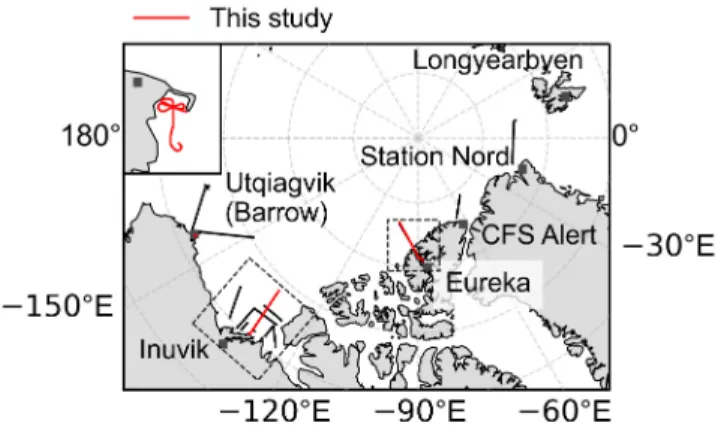
Fig. 2. Airborne surveys with the AWI Snow Radar between 2017 and 2019 (see Table II). The flight segments with the main focus in this article are highlighted in red, and the dashed squares indicate the extent of Figs. 9(a) and 10(a). The inset in the top-left corner shows a close-up of the short validation flight over the Elson Lagoon near Utqiagvik (Barrow) on April 10, 2017.

We have operated the AWI Snow Radar on three airborne campaigns over the Arctic sea ice in the Greenland, Lincoln, Beaufort, and Chukchi Seas and the Central Arctic Ocean (see Fig. 2 and Table II). In 2017, the Snow Radar was operated during six sea-ice survey flights as part of the Polar Airborne Measurements and Arctic Regional Climate Model Simulation Project (PAMARCMiP) [44], [45] from Eureka, Inuvik, and Utqiagvik (Barrow) between March 30 and April 10, 2017.

In the following year, we operated the Snow Radar over sea ice in the Fram Strait during a flight from Longyearbyen to Station Nord on April 10, 2018, as part of the campaign RESURV79 focused on surveying Nioghalvfjerdsbrae (79 N) Glacier in Greenland. Between April 1 and April 10, 2019, we did a total of seven survey flights with the Snow Radar from Eureka and Inuvik during the campaign IceBird Winter 2019, including areas in the Beaufort Sea not covered by OIB in that year.

During these deployments, we recorded over 980 000 radar returns.

Our analysis focuses on three individual flights on April 10, 2017, April 2, 2019, and April 10, 2019 (see Fig. 2 and Table II). The first flight has coincided within situsnow depth measurements carried out on landfast ice, which we used for validation. The surveys on April 2 and 10, 2019, contain long segments where flight tracks at two different survey altitudes overlapped. We used them for comparison to assess the effect of the survey altitude on the AWI Snow Radar measurements with the objective to quantify potential improvements of the low-altitude mode and evaluate the consistency with earlier OIB surveys.

C. Calibration

For calibration of the raw data, we used the MATLAB-based cresis-toolbox software provided by CReSIS [46], [47]. Fig. 3 illustrates the workflow that followed the same principle steps of methods applied previously to retrieve snow depth from Snow Radar waveforms [33], [40], [46], [48]. The first major step was the removal of altitude-independent coherent noise [visible in Fig. 5(a) below as undulating lines above the sea- ice surface]. Using a low-pass boxcar filter with a sampling frequency of 1/7.5 Hz and a cutoff frequency of 1/30 Hz,

TABLE II

AIRBORNESURVEYSWITH THEAWI SNOWRADAR(SEEFIG. 2)

we subtracted low-frequency along-track noise from the data resulting in only the high-frequency signal left in the data.

The next step was to analyze each data segment to detect specular targets by using an along-track discrete Fourier transform (DFT) over 512 range lines to extract the system response. Over the polar ocean and in calm wind conditions, we could use open water leads that were large enough (at least one Fresnel zone) as targets [48]. We detected sea-ice leads by comparing the coherent signal power in the 32 lowest frequency bins of the DFT with the incoherent power in the 425 highest frequency bins. When the power in the lowest frequency bins exceeded the power in the highest frequency bins by 25 dB, we further process that block of 512 range lines to extract a waveform representing the system impulse response. This is done by motion compensating each range line followed by taking an average over all of them to achieve a high signal-to-noise ratio impulse response estimate.

After collecting all the impulse responses from the blocks that satisfied the threshold, we tested the peak sidelobe ratio of each impulse response by deconvolving a sample range line from each block. We used the waveform with the lowest sidelobes for each segment to deconvolve that corresponding segment. If a data segment did not have any good waveforms

(5)

Fig. 3. Principal steps of the AWI Snow Radar data calibration and processing.

(e.g., segments were flown over MYI with few leads), then we manually chose impulse responses from another segment with corresponding nominal survey altitude. Usually, there were only a few sufficiently good impulse responses found for each segment, and some segments had no impulse responses extracted that improved the sidelobes.

To apply deconvolution, we convolved the radar data with the inverse of the extracted system response, which we limited to 400 range bins before and 150 range bins after the mainlobe with a Tukey window. We limited the range bin extent to reduce the amount of noise included in the impulse response and because this lowered the sidelobes in a large enough region around the mainlobe to prevent sidelobes from disrupting snow thickness tracking. Good system response deconvolution will suppress the range sidelobes [visible in Fig. 5(b)] and improve the 3-dB range resolution, which, in turn, will enhance the clarity of air–snow and snow–ice interfaces.

As part of deconvolution, we radiometrically calibrated the data so that the peak power was scaled to 1/R², whereRis the range. We used the impulse response with the lowest sidelobes as the calibration target. We assumed that the power reflection coefficient from this target (specular sea water surface) should be 0 dB. We scaled all the data products by the amount required to scale this calibration target to 0 dB. In addition, we narrowed the frequency window from 2–18 GHz to roughly half, 4–11.5 GHz, to avoid amplifying high-frequency noise.

As the final step, we applied elevation compensation to correct for changes in platform altitude and truncated the radar data frames to the default CReSIS radar sea-ice mission depth range of 8 m above and 5 m below the surface. We used the output of these two main steps, an unfocused synthetic aperture radar (SAR) quick look product of the vertically co-polarized channel (VV), as an intermediate product for our further analysis.

D. Processing

1) pySnowRadar: We identified air–snow and snow–ice interfaces from the calibrated Snow Radar echograms using the open-source pySnowRadar package [49]. Python-based pySnowRadar provides a modular framework to extract, transform, and load Snow Radar data. The generalized structure of the package allows for rapid development and validation of retrieval algorithms with parallel processing capabilities to scale with compute infrastructure. Originally developed to use the Haar wavelet interface detection method introduced in [32], pySnowRadar produces along-track snow depth estimates, which are largely insensitive to variations in mission-specific transmission power or receiver noise. However, methods described in [32] have not previously been validated for the 2–18-GHz bandwidth radar version of the Snow Radar used by the AWI. Early investigations with the Haar wavelet method revealed incorrect interface detection especially when

(6)

TABLE III

WAVEFORMPEAKDETECTIONPARAMETERS: POWERTHRESHOLDS(TH) IN THELOGARITHMIC(LOG)ANDLINEAR(LIN) SCALES,ANDLEFT-

HAND(L)ANDRIGHT-HAND(R) PEAKINESS(PP) THRESHOLDVALUES

the air–snow interface was the dominant scattering surface.

Therefore, to assess the suitability of this method, we developed a new interface picker module for comparison.

a) Peakiness method: Adapting an approach from satellite radar altimetry in [50], we used the concepts of left- and right-hand peakiness, PPl and PPr, respectively, to determine correct interface locations and disregard ambiguous waveforms. To detect the air–snow interface, we first identified all local maxima (peaks) that were above the mean noise level of the first 100 range bins by a user-defined peak detection power threshold in the normalized, logarithmic-scale waveform, whereas, for the snow–ice interface, we did the same but using normalized, linear-scale data to decrease the number of possible interface locations. In general, maximum return power was assumed to correspond to the snow–ice interface, i.e., the largest change in the dielectric properties. If more than five peaks above the peak detection power threshold were found in the linear data at this stage, the algorithm does not return any interface locations for the waveform in question because reliable interface signal cannot be retrieved but regards it as ambiguous. For each peak identified from the logarithmic (linear) data, we calculated the left-hand (right-hand) peakiness value using the mean of N preceding (succeeding) range bins in the linear normalized data as defined by [50]

PPl = s˜peak 1 N

N

i=1s˜_peak−i

·N (7)

PPr = s˜peak 1 N

N

i=1s˜peak+i

·N (8)

where ˜si =si/smaxis the normalized waveform in linear scale, i is the range bin index, and N is the number of range bins.

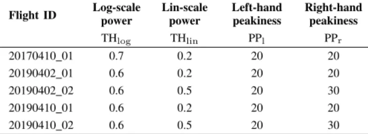
We chose N =10 for the calculations as it equaled two times the 3-dB range resolution (see Section III-A). We assigned the air–snow (snow–ice) interface to the first (last) peak identified from the logarithmic (linear) data that exceeded a user- defined left-hand (right-hand) peakiness value. An example of applying the method to a waveform is shown in Fig. 4. The four user-definable parameters described here were determined semiempirically through validation (see Section III-B) and random test frames from each segment to ensure consistency (see Table III).

2) Snow Depth Postprocessing: Following [32], we characterized the variability of the sea-ice surface within the radar footprint with the nonparametric surface topography estimate

htopo, which is defined as the difference of the 95th percentile and the 5th percentile of the surface elevation height:

htopo=h95−h05. (9) Here, we approximated the radar footprint to be circular with a radius corresponding to the theoretical smooth surface and cross-track footprint size. For the estimation ofhtopo, we used data acquired with the onboard near-infrared (1064 nm), fast line-scanning ALS (Riegl VQ-580), which has an accuracy and precision of 25 mm. Resulting WGS84 surface elevation point clouds were gridded into 0.25- or 0.50-m lateral resolution for the low and high survey altitudes, respectively [see Fig. 4(a)].

Following again the approach of [32], we set an upper limit of 0.5 m forhtopo where surface elevation data from the ALS were available. This was to include surface features on level ice, such as sastrugi, but to exclude potentially false snow depth estimates in the heavily deformed sea-ice environment.

We filtered out snow depth estimates that were acquired during the EM-Bird calibration maneuvers using a simple elevation threshold and when the absolute roll or pitch of the aircraft exceeded 5^◦. In addition, we regarded snow depths larger than 1.5 m as outliers and discarded them from further analysis.

E. Auxiliary Sea-Ice Data

To assist in the analysis and evaluate the results, we con- nected the snow depth estimates with coinciding multiyear ice fraction (MYIf) information using the 12.5-km resolution MYI concentration product from the University of Bremen [51], [52].

III. RESULTS

A. Calibration

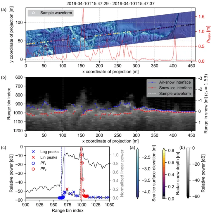
Fig. 5 shows how the radar data improved during the calibration process through coherent noise removal and system response deconvolution, which take place between the figure panels. Due to the lack of open water leads during some survey flights, not all segments could be deconvolved using specular targets from the same flight. However, in those cases, we used a deconvolution waveform from another segment with the same survey altitude, which may lead to reduced deconvolution quality due to drifts in the system response over time. Fig. 6 shows the system impulse deconvolution for the flight segments on April 10, 2019, which crossed several leads.

The reduction in bandwidth from 2–18 to 4–11.5 GHz during deconvolution [see Fig. 6 (Right)] prohibited amplifying high- frequency noise but caused an increase in the range resolution, which was evident also in the 3-dB range resolution that had a value of approximately 4.2 cm after deconvolution. While the deconvolution did not sharpen the main lobe significantly, the side lobes were suppressed to about −30 dB or less [see Fig. 6 (Left)].

To further investigate the effect of the system response deconvolution, we considered the system sidelobe strength dependence for our data both before and after deconvolution following [31], [33], and [53]. While they calculated the curves for the whole campaign (over 10⁶ waveforms), we restricted our analysis to individual flight segments due to the differing

(7)

Fig. 4. Example from the low-altitude survey flight 20190410_01 at approximately 71.36^◦N,−131.15^◦E. (a) Snow Radar derived snow depth estimates with the peakiness method (colored dots, footprint diameter has been exaggerated by a factor of 2) overlaid on ALS-derived WGS84 surface elevation (bluish swath). The red solid line is the corresponding along-track topographic variability (htopo), and the dashed line is its 0.5-m threshold (right-hand side vertical axis). (b) Corresponding section of the Snow Radar echogram with air–snow (blue) and snow–ice (red) interfaces identified with the peakiness method.

(c) Sample waveform [white circle in (a) and white dashed line in (b)] in logarithmic scale (black) and in linear scale (gray, right-hand side vertical axis) together with the air–snow (blue) and snow–ice (red) interfaces identified using the peakiness (solid line) and Haar wavelet (dashed line) methods. The blue (red) crosses and circles illustrate the left-hand (right-hand) peakiness calculation.

survey altitudes, thus limiting the total number of waveforms (in the order of 10⁴) in the resulting group of curves. The curves in Fig. 7 show radar returns that were oversampled by a factor of 16, averaged with a rolling window of the same size, and normalized with respect to the peak (maximum) return, ˜s(i)=s(i)/speak. We averaged them over 2-dB intervals of the peak signal-to-noise ratio, PSNR = speak/n,¯ where ¯n is the noise calculated from the first 100 range bins of the waveform. The figure shows the desired effect of reduced side lobes after deconvolution and also generally

higher SNR levels with lower altitude and for deconvolved data.

B. Validation

The last flight of the 2017 campaign on April 10 took place over a site with high-resolution and 2-D in situ snow measurements in the Elson Lagoon close to Point Barrow, Alaska. The ground-truth snow depth data were collected in a 650 × 450-m area surveyed using a terrestrial laser

(8)

Fig. 5. Example frame of the low survey altitude AWI Snow Radar data during different steps of the calibration process (a) before coherent noise removal, (b) after coherent noise removal, and (c) after system response deconvolution. Brighter colors indicate higher return power of the radar signal. The range axis is calculated assuming a snow density of 0.3 g·cm⁻³.

Fig. 6. (Left) Deconvolution waveforms and (Right) transfer functions for flight segments (a) 20190410_01 (low altitude) and (b) 20190410_02 (high altitude). The positive range axis is away from the radar.

scanner (TLS) to establish snow surface position relative to an array of 15 reference reflectors frozen to the ice on level landfast FYI on March 30–April 1, 2017. Snow depth was determined from the surface position by subtracting an ice surface that was presumed to be planar. The planar ice surface assumption, in this case, is well supported by scans of the snow-free ice surface in autumn, which showed less than 2 cm of surface height variation, a lack of vertical deformation in the

Fig. 7. Investigating system side lobes (a) before and (b) after the system response deconvolution for flight segments 20190410_01 (low altitude, left) and 20190410_02 (high altitude, right). Gray histograms show the probability distribution functions (pdf) of the snow depth estimates retrieved with the peakiness method with a bin size of 4 cm (right-hand side vertical axis). The range in snow is calculated assuming a snow density of 0.3 g·cm⁻³.

reference reflector array during the course of the winter, and cross comparison of the derived snow depths with probe-based measurements. The horizontal resolution of the resulting TLS field was 25 cm, and the vertical accuracy was determined to be approximately 1 cm by cross-comparison with manually measured snow depths collected with automatic snow depth probes (magnaprobe) within the survey area. The snow depth

(9)

in the entire area ranged from 1 to 71 cm with a mean value of 23 cm and a standard deviation of 6 cm. There was no precipitation and very little redistribution between the TLS and Snow Radar surveys. Prevailing winds from east to northeast affected the morphology of the dunes [see Fig. 8(i)].

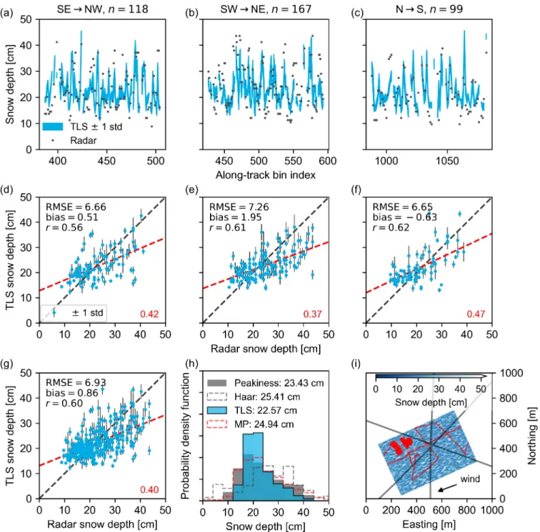
We surveyed the field site with the aircraft at the low survey altitude mode (200 ft) in three different directions: 1) from southeast to northwest; 2) from southwest to northeast; and 3) from north to south (see Fig. 8). For each radar return, we calculated the snow depth estimate using a snow density of 0.3 g·cm⁻³ derived from four snow pit profiles, which agreed also with the climatological value [20]. We determined the corresponding TLS snow depth as the mean value within a radius that we assumed to equal the theoretical smooth surface and cross-track radar footprint radius. To evaluate the validation, we calculated root mean square errors (RMSEs), mean biases, and correlation coefficients (r) for each crossing flight line separately and all overlapping points together.

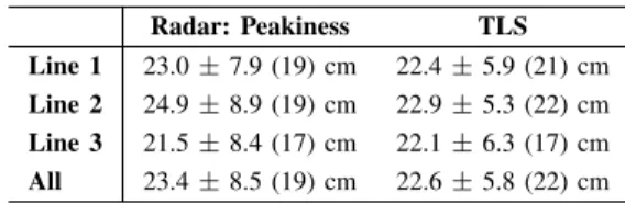
The validation results from the TLS comparison with the peakiness method are shown in Fig. 8 and Table IV. Bias in the comparison was minimized with peak detection power thresholds of 0.7 and 0.2 to detect the air–snow and snow–ice interfaces, respectively, and setting the threshold value to 20 for both peakiness parameters (see Table III), which retained 90% of the collected waveforms. Line 1 had the lowest correlation coefficient of 0.56, the shared-lowest RMSE of 6.66 cm, and a mean bias of 0.51 cm. Line 2 ran against the dominant orientation of the snow dunes and had the most values for comparison across the validation field. However, the results showed the largest values for RMSE and mean bias of 7.26 and 1.95 cm, respectively. Line 3 revealed a slightly negative bias (−0.63 cm), the best correlation coefficient out of the three crossing lines (0.62), and shared-lowest RMSE (6.65 cm). Considering all overlapping radar and TLS snow depth estimates together, we found a correlation coefficient of 0.60, an RMSE of 6.93 cm, and a mean bias of 0.86 cm, which was still well within the assumed TLS accuracy of 1 cm. The peakiness method well captures the snow depth distribution indicated by both the TLS and magnaprobe [see Fig. 8(h)].

On average, the validation of snow data picked with the Haar wavelet method showed worse results compared to the new picker method, despite retaining all waveforms, resulting in a correlation of 0.42 (ranging from 0.36 to 0.51 between the crossing lines), a mean bias of 2.57 cm (1.62–4.59 cm), and an RMSE of 10.26 cm (9.57–10.90 cm). The Haar wavelet method overestimated the mean snow depth by approximately 10% [see Fig. 8(h)].

We estimate the uncertainty by following the approach of [32] where the mean bias between the Snow Radar (SR) and TLS snow depths (δSR−TLS), the precision of the radar snow depths (εSR), and the precision of the TLS snow depths (εTLS) are added in quadrature:

σ_SR² =δ²_SR₋_TLS+ε_SR² +ε_TLS² . (10) Taking the 3-dB range resolution of 4.2 cm as the Snow Radar precision, the uncertainty results inσSR=4.4 cm (18% of the overall snow depth). This uncertainty value is lower than the

TABLE IV

MEAN± STANDARD DEVIATION(MODE)OF THEPEAKINESSMETHOD AND THETLS DERIVEDSNOWDEPTHESTIMATES INCENTIMETERS

FOR THEVALIDATIONSITE(SEEFIG. 8)

simplistic error estimate of 5.7 cm in [28] still being used for the current OIB snow depth on sea ice products [54], [55].

To this date, no further colocated AWI Snow Radar data and ground-truth measurements were available to us, neither were there flight tracks with colocated AWI and OIB Snow Radar data.

C. Intercomparison at Different Altitudes

Because of the differences in the nominal along-track spacing of the AWI Snow Radar data points between the two survey altitudes, the total number of high-altitude waveforms was 59% and 57% of the low-altitude waveforms for April 2 and 10, 2019, respectively. Therefore, we present the snow depth estimates averaged to 40-m and 1-km along- track bins. In Table V, the percentages show the fraction of valid waveforms after postprocessing (see Section II-D2) included in averaging. Due to the filtering according to the user-defined waveform parameter thresholds, the percentages for the peakiness method were consistently smaller than for the Haar wavelet method. In addition, due to the data gaps that resulted from the EM-Bird calibration maneuvers, we limited the snow depth comparison to those sections where estimates from both altitudes were available. We did not apply any drift correction nor adjust the flight track of the return segment.

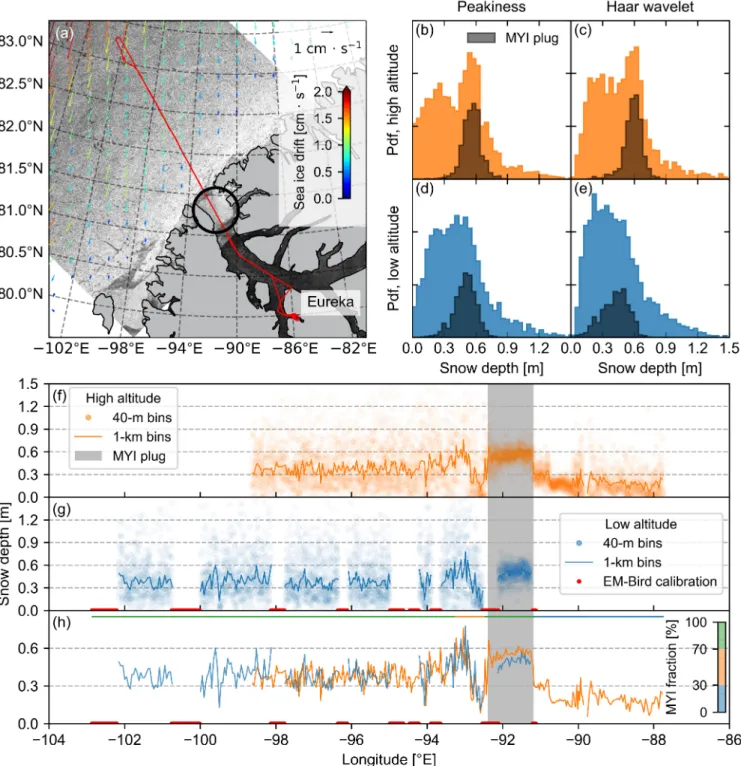
1) MYI: The flight on April 2, 2019, departed from Eureka along the Nansen Sound and out to the Arctic Ocean at the low survey altitude and returned at the high survey altitude [see Fig. 9(a)]. It was characterized by FYI in the Nansen Sound until a stretch of landfast MYI (a “plug”) several tens of kilometers in length right at the mouth of the sound, which is shown with a black circle in Fig. 9(a) around−92^◦E. After a short decrease in MYIf down to 40%, major parts of the segments were dominated by MYI only. The sea-ice drift of the surveyed area in the Arctic Ocean during that day was marginal, less than about 1.2 cm·s⁻¹ toward the south. Due to more turbulent conditions at the low survey altitude, we did not attempt to keep the exact overlap between the segment flight tracks. During the flight, the distance between the two segments was within 730 m with a mean of 250 m.

The retrieved snow depth distributions were mostly bimodal due to the continuously thick snow cover of around 0.5–0.6 m over the MYI plug; however, the bimodality was less clear in the low-altitude data and even absent in the corresponding Haar wavelet distribution [see Fig. 9(b)–(e)]. The mean snow depth (0.44 m) and standard deviation (0.26 m) using the peakiness method were consistent between the two survey altitudes, whereas the mean difference in snow depth of 0.06 m between the altitudes over the MYI plug mainly contributed

(10)

Fig. 8. Validation over the TLS snow depth field in Utqiagvik (Barrow) on April 10, 2017. The three columns are the flight paths crossing the field in three different directions: 1) from southeast (SE) to northwest (NW); 2) from southwest (SW) to northeast (NE); and 3) from north (N) to south (S).

(a)–(c) Along-track snow depth estimates derived from the radar and TLS data, whereas (d)–(f) show them as scatter plots with the calculated statistics in addition to the first-order least-squares fit lines and their respective slopes in red. (g) All overlapping snow depth estimates together (n=384) as a scatter plot and (h) their probability density functions using a bin width of 4 cm. For comparison, the snow depth distributions using the Haar wavelet method (gray dashed) and magnaprobe (MP, red dashed) are shown. The values in the figure legend correspond to the mean snow depths. (i) Overview of the validation site: the snow depth is shown with a range of bluish colors, the crossing flight tracks as black lines, and the magnaprobe measurements in red. The arrow shows the prevailing wind direction from east-northeast. The origin is at 4W 590250 7917600 in UTM coordinates.

to the differing modal values (see Table V). In comparison, the Haar wavelet method returned larger values for the mean and modal snow depth at the high survey altitude. For the low altitude, the mean snow depth and standard deviation were similar (0.43 and 0.25 m), but the missing second peak in the distribution resulted in a modal value of only 0.23 m.

Fig. 9(f) and (g) shows the snow depth estimate profiles derived using the peakiness method in 40-m and 1-km bins at the two survey altitudes. The 1-km averaged profiles follow

each other reasonably well considering that the flight tracks did not match exactly and no ice drift correction was done [see Fig. 9(h)]. However, we found a discrepancy over the MYI plug around −92^◦E. The 40-m binned snow depth estimates from the two survey altitudes showed the maximum correlation of 0.58 when the distance between the segments was up to 30 m and decreased to 0.2 and below when distance exceeded 300 m, and more values were included in the analysis. Similarly, RMSE was 0.14 m at small distances

(11)

TABLE V

TOTALALONG-TRACKDISTANCE(km), MODE(m), MEAN(m), STANDARDDEVIATION(m),ANDFRACTION OFVALIDPOSTPROCESSEDWAVEFORMS (wfs) INCLUDED INAVERAGING,AND NUMBER OF VALID40-m AVERAGED AWI SNOWRADARSNOW DEPTHESTIMATES FOR THETWO

ALGORITHMS AND FOR THELOW ANDHIGHSURVEYALTITUDEFLIGHTSEGMENTS ONAPRIL2AND10, 2019

and slowly increased to 0.3 m for distances larger than 500 m. A small negative bias of the low-altitude snow depth estimates, up to −0.1 m due to the difference over the MYI plug, eventually balanced out to near zero as the distance increased.

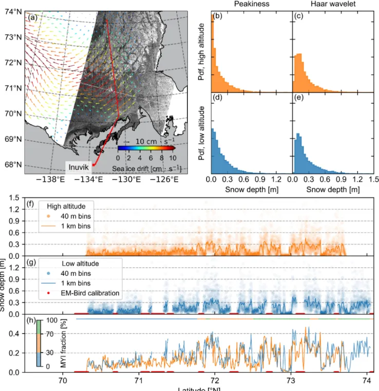
2) Mixed Ice Types: The flight on April 10, 2019, followed a ground track of the ICESat-2 satellite, namely, the ground track of the strong center beam of orbit number 189 of cycle 3, out to the East Beaufort Sea [57] [see Fig. 10(a)]. The flight path crossed several leads and varying types of ice: young and older FYI near the coast but also embedded in the MYI zone north of 71.75^◦N. Similar to the flight on April 2, we did the outbound survey at low altitude and returned at the high survey altitude. However, in more challenging flight conditions due to higher wind speeds, the maximum distance between the segments was 1.8 km and the average 460 m. Sea-ice drift velocity in this area on the day of the survey was up to one order of magnitude larger, around 10 cm·s⁻¹ with direction varying from south to southwest, moving the ice as much as 1.3 km during the 4-h survey.

Table V shows that the snow depth estimates at the low survey altitude were on average 0.03 m larger than at the high altitude. The same was true comparing the two retrieval methods, where the Haar wavelet method resulted in 0.06 m deeper mean snow depth estimates than the peakiness method.

The shapes of the distributions were similar, but the snow depths derived with the Haar wavelet included significantly less thin (<0.04 m) snow [see Fig. 10(b)–(e)], which was reflected also in the modal values.

The snow depth estimates derived using the peakiness method in 40-m and 1-km bins at the two survey altitudes are shown in Fig. 10(f) and (g). The 1-km averaged profiles captured the main features across the different ice types [see Fig. 10(h)]. However, compared to the profiles from April 2, snow depth estimates from the two survey altitudes differed more frequently, i.e., low altitude estimates exceeded the ones acquired from the high-altitude segment. This was because the radar measured inherently different snow due to the sea- ice drift between the overpasses as a function of temporal and spatial separations between the flight track segments over heterogeneous sea-ice conditions. The 40-m binned snow depth estimates from the two survey altitudes showed the maximum correlation of 0.40 when the distance between the low- and high-altitude segments was less than 40 m and decreased to 0.2 and below when including values that were separated by more than 620 m. Similarly, RMSE was 0.2 m at small distances and increased to 0.23 m for distances larger

than 600 m. A small positive bias of 0.06 m of the low-altitude snow depth estimates was eventually halved to 0.03 m as the distance increased.

IV. DISCUSSION

We have demonstrated the feasibility of sensor calibration for the AWI Snow Radar at the unprecedented low altitude of 200 ft, which included coherent noise removal and system response deconvolution using the cresis-toolbox (see Figs. 5–7). Previously, Yan et al. [48] showed the effect of coherent noise removal and system response deconvolution at the nominal 1500-ft survey altitude and found an improvement of 0.24 cm in the 3-dB range resolution. However, we did not find such an effect on our deconvolved sample data on either survey altitude. Moreover, they did not report any reduction in bandwidth that we were obliged to do to avoid amplifying high-frequency noise. We also think that the specularity of the sea-ice leads that we used as targets might have been compro- mised due to windy conditions and insufficient size. Using a man-made calibration target, for example, a corner reflector, as suggested in [48], would be a solution but logistically challenging. Future calibration steps include SAR-focused and array processing, which may further improve the radar data quality.

For the validation of our novel peakiness-based retrieval method, we compared the snow depth estimates derived from the AWI Snow Radar measurements at low survey altitude against 2-D in situ snow depth measurements from a TLS.

Mean values of 23.43 and 22.57 cm revealed an excel- lent agreement. The resulting slightly positive mean bias of 0.86 cm was well within the accuracy of the TLS snow depths and below radar sensor resolution. However, there were two main shortcomings to this validation. First, the range of TLS snow depths was narrow, only 31 cm. This lack of range likely reduced the obtained correlation between the data sets. For a more comprehensive validation, in situ snow depths with higher spatial variability are required. Second, the validation was limited to level landfast FYI, low survey altitude, and one season only. Due to weather constraints, further validation opportunities againstin situmeasurements on other ice types are not available to this date. For this reason, we chose to follow the approach of [32] and use the nonparametric surface topography estimate htopo to filter out potentially false snow depth estimates where the sea-ice surface was deformed.

We found that the new peakiness method worked better for the AWI 2–18-GHz radar version and low survey altitude

(12)

Fig. 9. Snow depth estimates over the Nansen Sound and the Arctic Ocean on April 2, 2019. (a) Flight track (red line) and Polar Pathfinder daily 25-km EASE-grid sea ice motion vectors [56] (colored arrows) overlaid on Sentinel-1 Level-1 extra-wide (EW) swath ground range detected (GRD) HH-polarized SAR images acquired on the day of the survey. Brighter colors indicate higher backscatter, i.e., rougher (older) sea ice. The black circle shows the location of the MYI plug at the mouth of the Nansen Sound. Copernicus Sentinel data 2019. (b) pdf of the 40-m averaged snow depth from the high-altitude segment using the peakiness method. The gray histogram shows the snow depth distribution over the MYI plug. (c) 40-m averaged snow depth pdf from the high-altitude segment using the Haar wavelet method. (d) and (e) Same as (b) and (c) but for the low-altitude segment. The bin width in the pdfs (b)–(e) is 4 cm. Basic statistics are given in Table V. (f) Along-track snow depth profile in 40-m (dots) and 1-km (line) bins using the peakiness method (the Haar wavelet method not shown) for the high-altitude segment against longitude. The gray section indicates the location of the MYI plug. (g) Same as (f) but for the low-altitude segment together with EM-Bird calibration maneuvers (red). (h) 1-km bin along-track profiles of the two segments combined together with MYIf classification.

than the Haar wavelet method. Although the retrieved snow depth estimates indicated similar statistics (see Table V and Figs. 9 and 10), the Haar wavelet method led to overestimation and underestimation of snow depth. As we showed in the validation (see Section III-B, Fig. 8) and further illustrated in Fig. 4(c), the Haar wavelet method overestimated the mean snow depth in a regular case where the snow–ice interface had

the largest return power. This was caused by the assumption of the method to assign the air–snow interface to the first range bin on the leading edge of the waveform that was above the noise floor, i.e., when the radar pulse began to illuminate the interface. This reflection could originate from the top of a sea-ice surface feature, such as a snow dune or a pressure ridge, and even from off-nadir [32]. Therefore, the

(13)

Fig. 10. Snow depth estimates over the East Beaufort Sea on April 10, 2019. For description, see the caption of Fig. 9. Note the different scales of the sea-ice drift in (a) and the different horizontal axes in (f)–(h). Basic statistics are given in Table V.

resulting snow depth estimate would correspond more to the maximum snow depth within the radar footprint rather than to the average. However, studies have shown that the air–snow interface may also be the dominant scattering surface in certain conditions and within the frequency range of the Snow Radar [58]–[60]. Consequently, the assumption of the Haar wavelet method to consider only points on the leading edge of the waveform [32] could lead to drastic underestimation of the snow depth when the maximum return power was associated already with the air–snow interface, while the signal from the assumed snow–ice interface was less powerful. The newly developed approach with peakiness parameters has been

specifically designed to picking correct interfaces also in such cases.

By design, the Haar wavelet method will not derive a zero snow depth as it considers two points on the leading edge of the waveform. Because we did not use any lead detection for filtering, in particular, the snow depth estimates derived with the Haar wavelet method on April 10, 2019, might be biased high. We also did not assign any limit, such as the theoretical or a multiple of the 3-dB range resolution [27], [32], for the minimum detectable snow depth to include the physical result of zero snow depth and to avoid biasing by excluding thin snow.

(14)

We acknowledge that the use of several user-definable peak detection parameter thresholds in the new peakiness method may introduce additional uncertainties and would ideally require validation in each season to constrain them properly. Our method decreases the sensitivity to the sea- ice surface features and the leading edge of the waveform compared to the Haar wavelet method, therefore bringing the derived snow depth estimates closer to the average value rather than the maximum. Increasing (decreasing) the peak detection threshold for the logarithmic power would decrease (increase) the snow depth as the air–snow interface is moved up (down) the leading edge of the waveforms. Varying the peak detection threshold for the linear-scaled power could allow more possible snow–ice interfaces to be detected especially when the air–snow interface is the dominant scatterer but, at the same time, risks increasing the number of ambiguous waveforms.

We think it would be worthwhile to further investigate if the parameter thresholds could be expressed as functions of surface roughness using data from the ALS. For example, the observed discrepancy in the snow depth estimates over the MYI plug [see Fig. 9(h)] indicates that assigning the thresholds for the peakiness method parameters dynamically based on ice type and radar footprint size rather than choosing constant values for each segment could improve the accuracy of the snow depth estimates. In addition, the detection of the air–snow interface could be improved by aligning the Snow Radar and ALS snow freeboard measurements, such as the approach of [27].

It is challenging to conclusively compare the overlapping flight segments with only centimeter-scale differences in the statistical values of the snow depth estimates without validation data on the ground. Considering the sea-ice drift, especially its cross-track component present during both flights [see Figs. 9(a) and 10(a)], and the distance between the segment flight paths, we think a direct comparison between flight segments is problematic.

In this article, we have demonstrated the viability of the AWI Snow Radar calibration and processing chains and that they are consistent with existing survey configura- tions. Together with the small radar footprint size, the high- resolution ALS data, and the new peakiness retrieval method, we are confident that the snow depth estimates presented here are of sufficient accuracy to derive snow depth on a regional scale for sea-ice mass balance and long-term monitoring.

V. CONCLUSION

Taking advantage of the slow speed and low altitude of the airborne AWI IceBird sea-ice surveys, we are able to measure sea ice with high spatial resolution. The quad- polarized 2–18-GHz FMCW microwave radar developed by CReSIS accurately measures snow depth on sea ice, and we have demonstrated that our new snow depth retrieval algorithm based on a signal peakiness parameter is capable to provide precise estimates of snow depth over different ice types and survey altitudes, even when the air–snow interface is the dominant scattering surface. The small radar footprint size at the low survey altitude of 200 ft enhances the spatial resolution and decreases the effect of off-nadir sea-ice surface features

compared to acquisitions at higher altitudes. The validation of low-altitude AWI Snow Radar data against a high-resolution 2-D TLS field, which resolves the snow depth distribution within the radar footprint but is restricted to level landfast FYI, is unique and yields a mean bias lower than the radar resolution. However, colocated Snow Radar and 2-D ground- truth surveys over different ice types are required to reduce the uncertainty of snow depth estimates in a deformed sea-ice environment. Comparison between the low and high survey altitudes of overlapping segments shows good consistency in the snow depth estimates derived with the peakiness method and, thus, data from the OIB program.

With the demonstrated capabilities of the AWI Snow Radar, we can now take advantage of the combined data sets of snow depth from the radar, snow surface freeboard from the ALS, and the total ice thickness from the EM-Bird. Linking them will enable us to describe the whole sea-ice layer on a regional scale as part of the long-term AWI IceBird program. Such information will be vital to facilitate studies of, for example, basin-scale snow depth and ice thickness assessment from dual-altimetry products in the era of CryoSat-2 and ICESat-2.

ACKNOWLEDGMENT

The authors acknowledge the use of the CReSIS toolbox from CReSIS generated with support from the University of Kansas. Wavelet-based retrievals described in this work were originally developed by the NOAA Laboratory for Satellite Altimetery and have been adapted for use in pySnowRadar.

They thank Kenn Borek Air, AWI technicians and logistics, Environment and Climate Change Canada (ECCC), and Cana- dian Forces Station (CFS) Alert, who helped at various stages of the data collection.

REFERENCES

[1] M. Webster et al., “Snow in the changing sea-ice systems,” Nature Climate Change, vol. 8, pp. 946–953, Nov. 2018.

[2] L. Kilic, R. T. Tonboe, C. Prigent, and G. Heygster, “Estimating the snow depth, the snow–ice interface temperature, and the effective temperature of Arctic Sea ice using Advanced Microwave Scanning Radiometer 2 and ice mass balance buoy data,” Cryosphere, vol. 13, no. 4, pp. 1283–1296, Apr. 2019.

[3] T. Markus and D. J. Cavalieri, “Snow depth distribution over sea ice in the Southern Ocean from satellite passive microwave data,” in Antarctic Sea Ice: Physical Processes, Interactions and Variability, M. O. Jeffries, Ed. Washington, DC, USA: American Geophysical Union, Mar. 1998, pp. 19–39.

[4] J. C. Comiso, D. J. Cavalieri, and T. Markus, “Sea ice concentration, ice temperature, and snow depth using AMSR-E data,”IEEE Trans. Geosci.

Remote Sens., vol. 41, no. 2, pp. 243–252, Feb. 2003.

[5] P. Rostosky, G. Spreen, S. L. Farrell, T. Frost, G. Heygster, and C. Melsheimer, “Snow depth retrieval on Arctic sea ice from passive microwave radiometers—Improvements and extensions to multiyear ice using lower frequencies,” J. Geophys. Res., Oceans, vol. 123, no. 10, pp. 7120–7138, Oct. 2018.

[6] N. Maaß, L. Kaleschke, X. Tian-Kunze, and M. Drusch, “Snow thickness retrieval over thick Arctic sea ice using SMOS satellite data,”

Cryosphere, vol. 7, no. 6, pp. 1971–1989, Dec. 2013.

[7] K. Guerreiro, S. Fleury, E. Zakharova, F. Rémy, and A. Kouraev,

“Potential for estimation of snow depth on Arctic sea ice from CryoSat- 2 and SARAL/AltiKa missions,” Remote Sens. Environ., vol. 186, pp. 339–349, Dec. 2016.

[8] I. R. Lawrence, M. C. Tsamados, J. C. Stroeve, T. W. K. Armitage, and A. L. Ridout, “Estimating snow depth over Arctic sea ice from calibrated dual-frequency radar freeboards,”Cryosphere, vol. 12, no. 11, pp. 3551–3564, Nov. 2018.