Plane wave expansion

Chapter 1

Photons in a cavity

Sketch of an optical cavity with a standing wave

1.1 Quantized electromagnetic fields

Expansion of cavity fieldsE andB: ‘separation of variables’

The amplitudesA1andA2are calledquadraturesin (quantum) optics. They play the same role as position and momentum coordinates in a harmonic oscillator. But which of them is ‘position’ and which one ‘momentum’ is less strictly defined and changes depending on the context.

Maxwell equations ⇒ relations between electric and magnetic mode functionsf(x)andg(x)and vector Helmholtz equation

Equations of motion = dynamics (time evolution) of the quadratures A1 andA2 (non-conventional notation! λis not a wavelength)

A˙2 =−kA1, A˙1 =c²λA2 (1.1) Translation table to harmonic oscillator of classical mechanics

(1.2) Quantization of the electromagnetic field in the cavity: in the same way as for the harmonic oscillator – translation table yields

Hˆ_osc = pˆ²

2m + kxˆ² 2 Hˆ = c²λAˆ²₂

2 + k

2Aˆ²₁ (1.3)

Key recipe for quantizing: correspondence principle= the Heisenberg equa- tions of motion must have the same form as the classical equations of mo-

tion d

dtAˆ2 = i

¯

h[ ˆH,Aˆ2] (1.4)

Work this out:

i

¯

h[ ˆH,Aˆ2] = i

¯

hAˆ1[kAˆ1,Aˆ2] =−kAˆ1 (1.5) provided the quadrature operators have the commutator

[ ˆA1,Aˆ2] = i¯h (1.6) which is consistent with the translation table (1.2).

stationary states (wave functions in the position representation) for the harmonic oscillator

energy levels for the stationary quantum states of the cavity field

The photon concept. Interprete the energy levels of the harmonic oscil- lator,En = ¯hωc(n+ ¹₂)as states with n packets of energy per photon, each packet havinghω¯ _c (Einstein and de Broglie). This works only for the har- monic oscillator where the energy spectrum is equidistant. In other words:

A photon is an elementary excitation of a mode of the elec- tromagnetic field. (70% of ‘Photon licence’ awarded by W. E.

Lamb.)

Note the shift away from ‘wave functions’ ψn(x) towards the slightly more abstract Dirac notation |n#with ‘ket’ and ‘bra’.

Creation and annihilation operators are built from the ‘ladder operators’

ˆ

aand ˆa^†of the harmonic oscillator spectrum:

Expression in terms of position and momentum coordinates ˆ

a ˆ a^†



= ˆx

$ k

2¯hωc ±i pˆ

√2¯hωcm, (1.7)

dimensionless operators with the commutator[ˆa,ˆa^†] = ˆ1(unit operator!).

Fix constants k and λ from the energy of the resonator mode. Corre- spondence principle: quantum-mechanical energy = sum of electric and magnetic field energy (both are integrals over energy densities).

Electric energy (density) Eel =

%

dxε0

2E²(x) = ε0A²₁ 2

%

dx|f(x)|²

& '( )

= 1

= ε0A²₁

2 (1.8)

where we have used a specific normalization for the mode function f(x).

The integral is finite because the mode is localized in the cavity (it is nor- malizable). Hence the correspondence principle fixes the constantk:

%

dxε0

2E²(x)=^! k

2Aˆ²₁ ⇒k =ε0 (1.9)

Magnetic energy

%

dx 1 2µ0

B²(x) = A²₂ 2µ0

%

dx|g(x)|² (1.10) This integral is linked to the previous one by the Maxwell equations

%

dx|g(x)|² = 1 k²

%

dx(∇ ×f)·(∇ ×f) = 1 k²

%

dxf·[∇ ×(∇ ×f)] (1.11) after a partial integration. The boundary terms involve the normal compo- nents of f ×(∇ ×f)and are zero for perfectly reflecting mirrors. Use the vector Helmholtz equation to get

%

dx|g(x)|² = kλ k²

%

dxf ·f = λ

k (1.12)

Therefore, we get again

%

dx 1 2µ0

B²(x) = A²₂λ 2µ0k

=! c²λAˆ²₂

2 ⇒k =ε₀ (1.13)

To improve the symmetry between electric and magnetic fields, we re-scale the magnetic mode g˜ = (k/λ)^1/2g such thatg˜ has the same normalization as f.

We end up with the following expressions for the electromagnetic quadraturesA1 and A2 in terms of the boson operatorsaanda^†:

a =A1

$ ε0

2¯hωc

+ iA2

$ c²λ 2¯hωc

(1.14) This yields the following expressions for the electric and magnetic field operators

E(x, t) =ˆ

$¯hωc

2ε0

(ˆa(t)f(x) + h.c.) (1.15) B(x, t) =ˆ −i

$¯hωcµ0

2 (ˆa(t)˜g(x)−h.c.) (1.16) These very important formulas describe in a precise manner the way classi- cal electrodynamics and quantum mechanics are linked in quantum optics and, more generally, in quantum field theory.

Classical properties: encoded in the mode function f(x), like frequency ωc. For a standing wave, the mode has no definite momentum. But a plane wave with wave vector kwould have that property. Similarly for the angular momentum which (already in classical electrodynamics) is a sum of orbitalangular momentum and spinangular momentum.¹

Quantum properties: one can only talk meaningfully about a photon cre- ated bya^†in the mode functionsf (andg). Its energy is˜ ¯hωc, its momentum would be¯hkif we are dealing with a plane wave. See the exercises for an expansion of a standing wave in momentum eigenstates.

Quantum field properties: the typical magnitude of the field ‘per photon’

is given by the square root

E1ph =

$ ¯hω_c

2ε0V (1.17)

where V is the ‘mode volume’ (related to the ‘size’ of f). The electric field (operator) is fluctuating around a zero mean value, even when there are no photons, with a magnitude of orderE^1ph. These fluctuations are a con- sequence of an uncertainty relation that exists in quantum field theory be- tween field (electric and magnetic) at nearby positions. In other words:

the fields are ‘grainy’ and are exchanged in energy packets (given by the famous¯hωc). The relevant packet size is a classical quantity and may even have some spread if the field is not a monochromatic mode.

In the following, no more hats on operators written down explicitly.

Plane wave expansion

For later use, we write down already here the expression for the field op- erators in free space, where an infinite number of modes contributes. A convenient basis is given by plane waves with wave vectors k and polar- ization vectors ekµ orthogonal tok, k·ekµ = 0 and normalized |ekµ|² = 1

1Orbital angular momentum: relates to derivative off, hence phase gradients. Exam- ples are helicoidal or vortex fields where the phase increases by 2π(or−4πwhen going around a zero of the field intensity). Spin angular momentum: related to circular polar- ization, hence the vector components of the field. Both angular momenta have integer quantum numbers because photons are bosons (not half-integer like electrons/fermions have).

(two possible values for the polarization index µ). If we restrict the mode functions to be periodic in a volume V, we have the natural orthogonality relation

%

Vd³xe^∗_kµ e^−ik·x

√V ·ek^!µ^!

e^ik!·x

√V =δµµ^!δkk^! (1.18) where the Kronecker symbolδkk^! makes sense because the periodic bound- ary conditions make the allowedk-vectors discrete. Thesameorthogonality relation is transferred to the photon operators akµ:

[a_kµ, a^†_k!µ^!] =δµµ^!δkk^! (1.19) The frequency of a plane wave mode is of course given by ωk=c|k|.

After these notations, we finally get the field operators E(x, t) =ˆ ^*

kµ

$ ¯hωk

2ε₀V

+ˆakµ(t)ekµe^ik·x+ h.c.^, (1.20)

B(x, t) =ˆ ^*

kµ

$¯hωkµ0

2V

+ˆakµ(t)bkµe^ik·x+ h.c.^, (1.21)

where the unit vectors for the magnetic field are given by (ω/c)bkµ =k× ekµ.

In the following, we come back to a single mode and discuss its dynam- ics and quantum states.

Dynamics

Heisenberg equation of motion for boson mode operator da

dt = i

¯

h[H , a] = iωc[a^†a+¹₂, a] = iωc[a^†a , a] (1.22) dynamics does not depend on zero point energy. Product rule for commu- tator with product yields

da

dt =−iωca , ⇒a(t) =a(0) e^−iωct (1.23) This equation of motion is just a complex combination of the two classical equations for the quadrature coordinates x and p. The form of the ex- ponential e^−iωct is similar to e^−iEnt/¯h for an energy eigenstate in quantum

mechanics. This has produced the namepositive frequency operatorfora(t).

More generally, we call the complex field operator

E⁽⁺⁾(x, t) =E1pha(t)f(x) (1.24) the positive frequency part of the field. The notation is confusing, as the term with the dagger a^† gives the negative frequency field E⁽⁻⁾(x, t). But the language has become established over the years.

Negative frequency solutions and antiparticles. Not a problem in clas- sical field theory: any real-valued field has both positive and negative fre- quency components. Electrodynamics, hydrodynamics etc.

Not a problem in quantum electrodynamics: in the negative frequency terma^†e^+iωct, the prefactor is interpreted as a creation operator of a photon, the same particle that is annihaled bya. This is generally true in elementary particle physics: a particle is its own antiparticle if its classical field is real (the quantized field becomes a hermitean operator).

In the quantized Dirac theory, for example, where a relativistic wave equation for the electron is quantized, the field operators for the electron are not hermitean. The prefactors of negative frequency solutions are in- terpreted as creating positrons, a different particle. Heuristically, one may interpret the creation operator of a position (anti-particle to the electron) as an annihilation operator for a particle in the ‘Dirac sea’ of filled negative frequency states.

1.2 Zoology of quantum states

1.2.1 Number (Fock) states

stationary states|n#,n = 0,1,2. . ., eigenstates ofnˆ =a^†a. Average field is zero because 'n|a|n#= 0.

Simple characterization (see coherent states in the next section): Q- or Husimi function defined on the complex plane α∈

Q_n(α) =|'α|n#|² = |α|²ⁿe^−|α|2

n! (1.25)

Circle around origin with radius|α| ∼√n. Easy to remember: no preferred phase on the ellipse (circle) of a constant-energy surface. See Fig.1.3 below.

1.2.2 Coherent (Glauber) states

denoted|α#withα∈ . Eigenstates of annihilation operatora|α#=α|α#. Coherent states are those that come closest to ‘classical electrodynam- ics’:

'α|E(x)|α# *= 0 (1.26) Therefore, they are often used as the (lowest-order) approximation to the state of a laser. More details, see exercises.

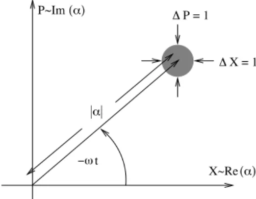
Δ Δ

X = 1 P = 1

X~Re P~Im

(α) (α)

t

|α|

−ω

Figure 1.1: Illustration of a coherent state in the phase-space plane. Here, the actual ‘size’ of the state, here equal to 1 in diameter, depends on the probability distribution that is used. We use here the Q- or Husimi func- tion. See Fig.1.3 where also a number (Fock) state and a squeezed state is plotted.

Minimum uncertainty state: check quadratures Xθ = ae^−iθ+a^†e^iθ

√2 , [Xθ, Xθ+π/2] = i (1.27)

and (exercise)

'α|∆X_θ²|α#= 1

2 (1.28)

(exercise) definition of normal order and:X_θ²: =X_θ² +. . .

Time evolution of a coherent state: use the expansion in Fock states and the solution to the time-dependent Schr¨odinger equation (N: normaliza- tion factor)

|α(t)# := e^−iHt/¯h

*∞ n=0

N αⁿ

√n!|n#=

*∞ n=0

N αⁿ

√n!e^{−iωc(n+12)t}|n#

= e^−iωct/2|αe^−iωct# (1.29) The phase factor e^−iωct/2 involving the zero-point energy is often dropped by shifting the zero of energy so that the ground state |0# has energy zero, H +→¯hωca^†a.

We thus see that under time evolution, a coherent state with parameter α transforms into another one with αe^−iωct: the ‘state is rotating’ in the complex plane. In other words, the set of coherent states is ‘closed’ under time evolution. This rotation is the same as the motion of a classical oscilla- tor in phase space along an ellipse of constant energy. The analogy will be pushed further when we introduce phase-space quasi-probability densities for quantum states. The coherent states play an important role for these probabilities.

1.2.3 Classical sources generate coherent states

A ‘classical source’ is a time-dependent term that is added to the Hamilto- nian:

H(t) = ¯hωca^†a+J(t)a^†+J^∗(t)a (1.30) If J(t) is real, this source can be interpreted as a force because it couples to the displacement coordinate X = (a^†+a)/√

2. We thus study a driven quantum oscillator.

Let us focus on the simple case of a monochromatic driving where J(t) =Je^−iωLt. The notationωLis inspired from a laser field that is coupled to the cavity mode via one of the mirrors. The amplitude J thus contains both the laser field amplitude and the mirror transmission coefficient. The Hamiltonian becomes

H(t) = ¯hωca^†a+Ja^†e^−iωLt+J^∗ae^iωLt (1.31)

We show in the following that after a time t, this Hamiltonian creates out of the vacuum state a particular coherent state

t= 0 : |0# +→t: e^iϕ(t)|α(t)# (1.32) with functions ϕ(t)andα(t)that are given below. In other words: under a Hamiltonian with linear and bilinear terms inaanda^†, coherent states evolve into coherent states. We shall see exceptions to this rule later, in particular when we are dealing with an ‘open cavity’ where photons can enter or leave the cavity.

First step: get rid of the time dependence by a unitary transformation.

This is called ‘switching to the rotating frame’. We write the state of the system in the form

|ψ(t)#=UL(t)|ψ(t)˜ #, UL(t) = exp(−iωLa^†a) (1.33) and find for |ψ(t)˜ #a Schr¨odinger equation (exercise!)

i∂_t|ψ(t)˜ # = H_rf(t)|ψ(t)˜ #

Hrf(t) = U_L^†(t)H(t)UL(t)−i¯hU_L^†(t)∂tUL(t) (1.34) This result is in fact quite general and holds for any time-dependent unitary transformation. Working this formula out in the rotating frame, we find thatH_rf is time-independent. This happens because the samefrequencyω_L appears in the source term of H(t) [Eq.(1.31)] and in UL(t) [Eq.(1.33)].

We find (exercise!)

Hrf = ¯h(ωc−ωL)a^†a+Ja^†+J^∗a (1.35) In the following, we use the notation ∆L = ωL− ωc for the detuning of the laser relative to the cavity resonance. (Attention: conventions with the opposite sign also appear. We adopt here the ‘Paris convention’ used by the group of Cohen-Tannoudji at theEcole normale sup´erieure= ENS.)

Second step. SinceH_rf [Eq.(1.35)] is time-independent, the time evolu- tion operator is easy to write down:

Urf(t) = exp(−itHrf/¯h) = exp[it(∆La^†a−(J/¯h)a^†−(J^∗/¯h)a)]

= exp[i∆_Lt(a^†−γ^∗)(a−γ)]e^{−i|γ2|∆Lt} (1.36)

with the shorthandγ =J/¯h∆L. Technique: displacement operator

D(α) = exp(αa^†−α^∗a), D^†(α)aD(α) =a+α (1.37) Can be proven with a differential equation (exercise!). For any operator functionf(a, a^†)with a polynomial expansion

D^†(α)f(a, a^†)D(α) = f(a+α, a^†+α^∗) (1.38) Link to coherent states: ‘displace the vacuum state’, i.e., D(α)|0# = |α#. Can be shown Eq.(1.37) up to a sign. D(α) is a unitary operator because D^†(α) = D⁻¹(α) =D(−α).

With the displacement operator, we can re-write

exp[i∆Lt(a^†−γ^∗)(a−γ)] = D^†(−γ) exp[i∆Lta^†a]D(−γ) (1.39) Now we can put everything together. Let us assume that we start with the vacuum state|0#at t= 0. The state at timetis:

|ψ(t)# = UL(t)Urf(t)|0# Let us first analyze the state in the rotating frame

|ψ(t)˜ # = Urf(t)|0#=D^†(−γ) exp[i∆Lta^†a]D(−γ)|0#e^{−i|γ2|∆Lt}

= D(γ)|−γe^i∆Lt#e^{−i|γ2|∆Lt} (1.40) Now we need the composition law (Hintereinanderausf¨uhrung) of displace- ment operators (exercise!):

D(α)D(β) = e^{−i Imα∗β}D(α+β) (1.41) for α = γ and β = −γe^i∆Lt. We finally get a coherent state with a phase factor

|ψ(t)˜ # = e^{i Im(γ∗γei∆Lt)}|γ(1−e^i∆Lt)#e^{−i|γ2|∆Lt}

= e^{−i|γ2|(∆Lt−sin ∆Lt)}|γ(1−e^i∆Lt)# (1.42)

In the case of exact resonance between laser and cavity, we have ∆L = 0, and one generates a coherent state with an amplitudeγ(1−e^i∆Lt)→ −iJt/¯h that increases linearly witht. (Exercise: makes sense for realJ.)

Apply the rotating frame operatorU_L(t)is easy (exercise).

Exercise: plot the ‘path’ in complex plane.

Going back from the rotating frame:

|ψ(t)#= e^iϕ(t)|γ(e^−iωLt−e^−iωct)# (1.43) with a phaseϕ(t) =|γ²|(sin ∆Lt−∆Lt).

Remark. On the role of time ordering. The time evolution operator for the Hamilto- nian (1.31) is

U(t) = T exp-(−i/¯h)% t 0

dt^"H(t^"). (1.44)

where ‘T’ means time-ordering, i.e.: ‘in the series expansion of the exponential, order operator products likeH(t1)H(t2). . . such that the time arguments are chronologi- cal t1 ≥ t2 ≥ . . .’. This prescription is necessary to get the correct solution to the Schr¨odinger equation. If we ignore this prescription, we get the quite different result U(t)≈exp-

−iωcta^†a−(J/¯hωL)a^†(1−e^−iωLt) + (J^∗/¯hωL)a(1−e^iωLt).

(wrong) Note in particular that the detuning∆L does not appear here. Let us instead switch to the so-called interaction picture. We split off the unitaryU0(t) = exp [−iωcta^†a]for the free cavity and get an effective Hamiltonian

Hint(t) =Ja^†e^−i∆Lt+J^∗ae^i∆Lt (1.45) where only the interaction with the classical driving remains. As in Eq.(1.44), we perform again the time integration without taking care of the time ordering, and get (recall thatγ=J/(¯h∆L)

Uint(t)≈exp-

γ a^†(e^−i∆Lt−1)−γ^∗a(e^i∆Lt−1).

(1.46) which is, indeed, a displacement operator with parameterγ(e^−i∆Lt−1). Apply to the vacuum (initial) state and go back to the standard picture, we find:

|ψ(t)# ≈ |γ(e^−iωLt−e^−iωct)# (nearly OK) (1.47) which is the same coherent state as in Eq.(1.43),exceptfor the phase factore^iϕ(t)that is missing. Note that the phase is like Berry’s geometric phase and multiplies the state vector. Note also that it is higher order in∆Lt, it vanishes on resonance. In usual averages, this phase factor drops out, unless one takes an interference setting where a superposition of different initial states is prepared.

Phenomenological damping

As mentioned in the introduction, quantum optics is the field where damp- ing and loss play a role for quantum systems. Several techniques have been developed and will be touched upon in this lecture. We start with the simplest model for theloss of photonsoutside the cavity.

We consider only the Heisenberg picture for the moment. One intro- duces additional terms in the equations of motion of an operatorA:

d

dt'A#= i

¯

h'[H , A]#+1 2

*

κ 'L^†_κ[A , L_κ] + [L^†_κ, A]L_κ# (1.48) where the operatorsLκact on the Hilbert space of the system and are called

‘quantum jump’ or Lindblad operators. For brevity, we do not present a detailed derivation of this equation for the moment, but just make a few remarks.

• The Lindblad–Heisenberg equation (1.48) preserves the properties of ex- pectation values for physical states (linearity, positivity etc.)

• Eq.(1.48) is based on the so-called Markov approximation where the knowledge of (average) operators at time t is sufficient to predict the fu- ture.

• The Lindblad-Heisenberg equation is in general only valid for operator averages. Similar equations at the operator level may require a different structure.

In the case of photons that escape from a cavity, a single Lindblad oper- ator is sufficient

L=√

κ a (1.49)

where ais annihilation operator and κa positive parameter with the units of a rate. This formula is easy to remember if we interpret Las a ‘quantum jump’: the system jumps to a state with one photon less.

Working out the equation of motion for the cavity operator A = a, we get (exercise) for a cavity with loss rateκand a driving laser with amplitude J(t):

d

dt'a#=−iωc'a# − i

¯

hJ(t)− κ

2'a# (1.50)

The last term leads to the damping of the cavity field with a rate κ/2. We can thus identify the prefactor of the Lindblad operator L with the cavity loss rate. (Different conventions: κ/2orκfor the damping of the field.)

Discussion: introduce quadratures [Eq.(1.27) and exercises]a = (X+ iP)/√

2and separate Eq.(1.50) into real and imaginary parts.

d

dt'X#= +ωc'P#+ 1

¯

hImJ(t)− κ 2'X# d

dt'P#=−ωc'X# − 1

¯

hReJ(t)− κ

2'X# (1.51)

The terms involving ωc correspond to the classical oscillator dynamics. If J(t) is purely real, then it acts like a force on the momentum quadrature P. If it is complex, the driving couples to both ‘position’ and momentum.

(Hence, strictly speaking,X is not a ‘position’ quadrature.) Finally, the lin- ear damping proportional toκacts on bothposition and momentum – this again is a hint that the phenomenological prescription with the Lindblad operator (1.49) cannot be exactly true. It is OK if the damping is weak (slowly enough) so that it acts only on time scales much larger than 1/ωc

(the free cavity period). In this situation, one cannot distinguish whether the damping affects momentum or position, since the two are rapidly ex- changing role on the time scale 1/κfor the damping.

We shall later that a cavity with this type of damping evolves in time from a coherent state to another one. If there is no driving, the cavity relaxes on a time scale1/κto the vacuum state|0#with zero photons. In the presence of monochromatic driving, the cavity reaches the coherent state|γ(∞)#with

γ(∞) = J

¯

h(∆L−iκ/2)

1.2.4 Thermal (Boltzmann) states

Example of a ‘statistical mixture’. Combines classical statistics (Boltzmann probabilities) with quantum averages (expectation values for observables).

Thermal states are built from the eigenstates (stationary states) of an en- ergy operator (Hamiltonian). If we take H = ¯hωc(a^†a+ ¹₂), then the sta- tionary states are the Fock states |n#, eigenstates to the photon number operatornˆ=a^†a. The Boltzmann weightpT(n)for this state is given by the classical statistics rule:

p_T(n)∼exp(−E_n/k_BT) (1.52)

where En = (n + ¹₂)¯hωc is the energy of the stationary state and T the temperature. We introduce the abbreviation β = ¯hωc/kBT. The probabil- ities in Eq.(1.52) must be normalized: this requires that the spectrum H be bounded from below and that the partition function (Zustandssumme) Z converges:

Z =

*∞ n=0

exp(−En/kBT) = e^−β/2

1−e^−β = 1

2 sinhβ/2 (1.53) One may introduce the free energy (log is the natural logarithm, often de- notedln)

Z = e^−F/kBT , F =−kBT logZ =kBTlog(2 sinhβ/2) (1.54) and derive from it the mean energy'H#, the entropyS etc (exercises!)

'H# = −¯hωc

∂

∂β logZ =. . . S = −∂F

∂T =. . . (1.55)

Exercise: identify the contribution of the zero-point energy to these quan- tities. (For the comparison, you can simply shift the energy eigenvalues E_n.)

Density operator, averages

How are expectation values calculated in a thermal state? Consider an observableAand work out its average in a stationary state'A#ⁿ='n|A|n#. Then these ‘quantum averages’ are averaged ‘in the classical sense’ with the probabilitiespn(T):

'A#T =^*

n

pT(n)'n|A|n#=^*

n

pT(n)'A#n (1.56) An equivalent way is to introduce the so-called density operator ρ: an op- erator acting on the Hilbert space of the system that is defined by

ρ= e^−H/kBT

Z (1.57)

In our case, the eigenstates of H are the Fock states, and we can give the explicit spectral representation:

ρ=^*

n

e^−En/kBT

Z |n#'n|=^*

n

pT(n)|n#'n| (1.58) This sum over projectors|n#'n| with positive probabilities as coefficients is called a ‘mixture’ or ‘convex mixture’.

The word ‘convex’ arises from the topology of sets. Take two pointsAandBin a set and form the straight line that connects them

x=pxA+ (1−p)xB, 0≤p≤1

The set is convex when it also contains this line. In the picture above, the set is not convex, as can be seen from the dotted line. In axiomatic quantum mechanics, the set of density operators is convex: given two density operatorsρA andρB, also their mixtures (the ‘line in between’) are physical states. The pure states appear as ‘extremal points’ in this convex set.

Once the density operator is known, expectation values for observables A are calculated from the so-called trace formula

'A#= tr (Aρ) (1.59)

This formula is true as long as ρ is normalized to unit trace: trρ = 1.

Calculations are actually easier because the trace can be worked out in any basis. Exercise: show that this is equivalent to Eq.(1.56). Show thatρdoes not depend on the zero-point energy.

Axiomatic approach: positive operator, trace-class, pure vs non-pure states, purity, von Neumann entropy, Hilbert-Schmidt scalar product.

Phase space picture

In the plane spanned by the quadratures X and P, a thermal state with density operatorρT can be characterized by taking the expectation value

Q_T(α) ='α|ρ_T|α#= tr (|α#'α|ρ_T) (1.60)

Calculate this

Q_T(α) = ^*

n

p_T(n)|'n|α#|²

= (1−e^−β)^*

n

e^−βn|α|²ⁿe^−|α|2 n!

= (1−e^−β) exp [−|α|²(1−e^−β)] (1.61) . . . a gaussian centered at α = 0 zero with a width 1/(1−e^−β) = ¯n+ 1 where n¯ = 'nˆ#T is the average thermal photon number (also known as Bose-Einstein statistics).

Exercise: work out so-called Wigner function, defined as the expecta- tion value of the displacement operator

WT(α) ='D(α)#= tr[D(α)ρT] (1.62) Result: zero-centered gaussian with width ¯n+ ¹₂.

Preparation of a thermal state

In quantum optics, the density operator is very often used. The reason is that one deals with systems that must be described statistically. For exam- ple: one cannot predict when a photon or how many photons will leave a cavity mode. To describe the time evolution, one is setting up equations of motion for the density operator (or matrix). These equations of motion are sometimes phenomenological, similar to the damping scheme for the cavity we found above. There are also quite accurate approximation schemes that lead to so-called master equations. We introduce here a simple example, called a set of ‘rate equations’.

The basic quantities in a rate equation are probabilities of finding the system in certain states. We take here the number (Fock) states. The prob- ability is a diagonal element of the density matrix:

pn(t) ='n|ρ(t)|n#. (1.63) It is a real number 0 ≤ pn ≤ 1thanks to the defining properties of a den- sity operator. The time argument t indicates that we are working in the Schr¨odinger picture where the (generalized) state ρ(t)changes in time.

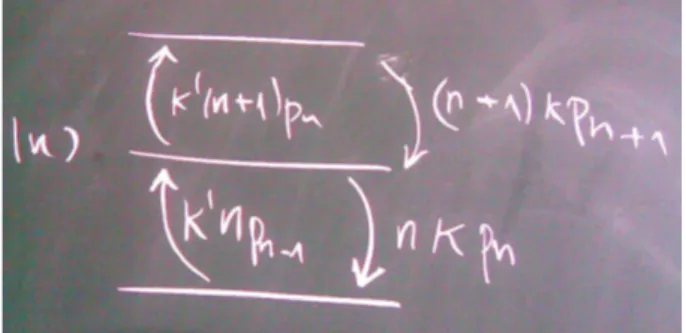
Figure 1.2: Illustration of transitions between states of the cavity with n and n±1photons.

The rate equations are differential equations dpn

dt =−κnpn+κ^$npn−1−κ^$(n+ 1)pn+κ(n+ 1)pn+1 (1.64) The constantsκandκ^$can be interpreted as transition rates between states (see Fig.1.2): the transition |n# → |n−1# happens with the rate κn(this rate appears as a negative term in p˙n and as a positive term inp˙_n−1). This process can be interpreted physically as the loss of one of the n photons.

This photon goes into a ‘thermostat’ or ‘environment’ and is absorbed there.

Similarly, the system described by ρˆcan absorb one photon from the ther- mostat – this happens with a ‘Bose stimulation factor’ because for the tran- sition |n −1# → |n#, the rate is κ^$n. (To be read off from the second and third terms in Eq.(1.64).) Even the vacuum state can absorb a photon, hence notn−1, butnappears here.

If one waits long enough, the density matrix (more precisely, its diago- nal elements) relaxes into a steady state given by the equations of ‘detailed balance’

0 = −κnp^(ss)_n +κ^$np^(ss)_n−1

0 = −κ(n+ 1)p^(ss)_n+1+κ^$(n+ 1)p^(ss)_n (1.65) These equations imply that p˙n = 0 in Eq.(1.64), but they are slightly stronger. (One can show them by induction, starting fromn = 0.) Eq.(1.65) gives a recurrence relation that linksp^(ss)_n top^(ss)_n−1, whose solution is

p^(ss)_n ∼

/κ^$ κ

0n

=: e^{−n¯hω/kBT} (1.66)

where we can identify the temperature T from the ratio of the rate con- stants κ^$/κ. (One needs κ^$ < κ, otherwise, no stable equilibrium state is found.)

Of course, this definition of temperature is linked to assigning an energyn¯hωto the state|n#. In other words: if we have the stationary populations that follow a power lawpn ∼qⁿ, then this determines only theratiobetween the temperature and some cavity Hamiltonian proportional to the photon number:

¯ hωc

kBT =−logq

In other cases, it may happen that the density operator is diagonal in a different basis, and that one may not even coincide with the eigenstates of the system Hamiltonian:

it suffices that the ‘dissipative’ terms of the master equation are large enough.

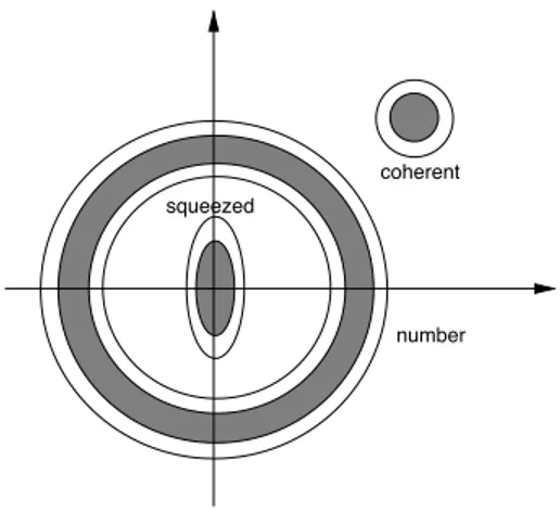
number squeezed

coherent

Figure 1.3: Illustration of different quantum states in the phase-space plane. We plot here the Q- or Husimi function that is positive everywhere.

The thermal state is centered at zero and has a width (area) larger than the coherent state.

1.2.5 Squeezed states

We have seen in a few places that the quantum character of the resonator mode becomes visible in the (‘quantum’) fluctuations around classical mean values. So people have thought whether it is possible to reduce the fluctu- ations in one field quadrature to get something even ‘more classical’ – i.e., having less noise. This can be achieved in part, to 50%, say. Of course, one cannot beat the Heisenberg inequality, and we shall see that the reduced

fluctuations in one quadrature have to be paid by enhanced noise in the other one.

Figure 1.4: Illustration of squeezed states in the phase-space plane.

A qualitative picture of squeezed states is given in Figs.1.3 and 1.4. They are characterized by quadratures x^$ and p^$ (typically rotated with respect toX andP such that their fluctuations are

∆x^$ = ∆X_φ< 1

√2, ∆p^$ = ∆X_φ+π/2 > 1

√2 (1.67)

The product is nevertheless compatible with the Heisenberg relation,

∆x^$∆p^$ = 1

2 (1.68)

so that squeezed states are minimum uncertainty states (as are the coherent states, for examples) with respect to quadrature measurements.

One may also have (see Fig.1.4) displaced squeezed states such that their photon number (or ‘intensity’) has reduced fluctuations (the refer- ences value would be the Poisson limit ∆n = 'n#^1/2 for a coherent state).

The price to pay are enhanced phase fluctuations. (For a discussion on the phase operator in quantum optics, see the book by Vogel & al. (2001).) Such states are interesting in applications where the intensity of a light beam should be ‘as stable as possible’. An example is a gravitational wave detector where light beams are reflected by mirrors: the radiation pressure of the beam pushes the mirrors (proportional to the intensity) and this dis- placement should be little noisy as possible, otherwise it obscures the path length differences due to gravitational waves.

Squeezing in theory

Let us consider the following unitary operator

S(ξ) = exp⁺ξa^†2−ξ^∗a^2, (1.69) Its action on the operators a and a^† is the following linear transformation (also called Bogoliubov or squeezing transformation)

a+→S(ξ)a S^†(ξ) =µ a−ν a^† (1.70) a^† +→S(ξ)a^†S^†(ξ) =µ a^†−ν^∗a

where the squeezing parameters are

µ= cosh(2|ξ|), ν = e^iφsinh(2|ξ|), φ = arg(ξ) (1.71) To prove Eq.(1.70), one makes the replacement ξ +→ ξt and derives a dif- ferential equation with respect to the parameter t. (Mathematically: one studies the one-parameter family of squeezing operators S(ξt), a subgroup in the group of unitary transformations.)

The squeezed state|ξ#is now defined as the ‘vacuum state’ with respect to the transformed annihilation operator:

0 = S(ξ)a S^†(ξ)|ξ# (1.72) This equation combined with the assumption that the vacuum state defined bya|vac#= 0is unique, gives|vac#=S^†(ξ)|ξ#after fixing a phase reference and therefore

|ξ#=S(ξ)|vac# (1.73)

because S^† is inverse to the unitary operatorS. We thus get the squeezed state by applying the squeezing operator to the vacuum state.

One can also discuss more general cases, for example a squeezed coherent state

|ξ, α# = S(ξ)|α# = S(ξ)D(α)|vac#. See the book by Vogel & al. (2001) for more details.

The photon number distribution for a squeezed state is interesting. Con- sider first the case of a small squeezing parameter ξ. The expansion of Eq.(1.73) yields

|ξ#= ( +ξa^†2−ξ^∗a²+. . .)|vac#=|vac#+√

2ξ|2#+. . . (1.74)

so that in addition to the ordinary vacuum, a state with a photon pair appears. This is a general feature: the squeezed (vacuum) state|ξ#contains pairs of photons,|2#,|4#, . . . We shall see below that this can be interpreted as the result of a nonlinear process where a “pump photon” (of blue color, say) is “down-converted” into a pair of red photons. The unusual feature of this “photon pair state” is that the pair appears in a superposition with the vacuum state, with a relative phase fixed by the complex squeezing parameter ξ.

To get the full expansion of the ‘squeezed vacuum’S(ξ)|0#in the Fock (number state),

|ξ#=*

n

cn|n#

it is most easy to write out Eq.(1.72):

0 =S(ξ)a S^†(ξ)|ξ#= (µ a−ν a^†)|ξ#

This gives a recurrence relation between the amplitudescn. One finds that only even photon numbers contribute with amplitudes

c0= 1

cosh^1/2(2|ξ|), c2m= (2m−1)!!

1(2m)! e^imφtanh^m(2|ξ|)

cosh^1/2(2|ξ|), m= 1,2. . . whereφis again the phase ofξ, andn!!is the productn(n−2)· · ·of all positive num- bers with the same parity up ton. The factorcosh^−1/2(2|ξ|)ensures the normalization:

it is the most difficult part to calculate.

Properties of squeezed states

The squeezed state has a mean photon number

'ξ|a^†a|ξ#='vac|S^†(ξ)a^†aS(ξ)|vac#=· · ·=|ν|² (1.75) as can be shown by applying the transformation inverse to Eq.(1.70) (re- placeξ by−ξ).

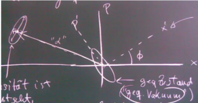
The mean value of the complex field amplitude is zero in the squeezed state, as a calculation similar to Eq.(1.75) easily shows: 'ξ|a|ξ# = 0. In the phase-space plane introduced in Fig. 1.1, the squeezed state|ξ#would therefore be represented by a “blob” centered at zero.

The “squeezing” becomes apparent if one asks for the quantum fluc- tuations around the mean value. For the general quadrature operator [Eq.(1.27)]

Xθ = ae^−iθ+a^†e^iθ

√2

The squeezed state now has fluctuations around the vacuum state such that one quadrature component has quantum noise below the Heisenberg limit1/2.

A straightforward calculation gives the following quadrature uncertainty 'ξ|∆X_θ²|ξ#= |µ+νe^−2iθ|²

2 (1.76)

If we take 2θ = φ (the phase of the squeezing parameter), we have µ+ νe^−2iθ = cosh(2|ξ|) + sinh(2|ξ|) = e^+2|ξ|which becomes exponentially large as the magnitude of ξ increases. For the orthogonal quadrature, one finds an exponential reduction of the fluctuations:

∆X_φ/2² = e^+2|ξ|

2 , ∆X_(φ+π)/2² = e^−2|ξ|

2 . (1.77)

This is the hallmark of a squeezed state. Note that the uncertainty product is unchanged: this could have been expected as |ξ#remains a pure state.

A graphical representation is shown above (see also Fig. 1.3) where the squeezed state is the ellipse centered at the origin. As discussed for Fig. 1.1, this picture can be made more quantitative by calculating certain phase-space distribution functions for the different states discussed so far.

This topic will be discussed in detail in part II of the lecture, the main results appear in Sec.??below.

Preparation of a squeezed state

How can one prepare a squeezed state? The “cheating way of it” is just a re-scaling of the position and momentum quadratures:

X^$ =ηX, P^$ =η⁻¹P (1.78)

This generates operators X^$ and P^$ that obey the same commutation rela- tions. However, the energy of the field mode will not be proportional to

a^$†a^$ ∼ X^$2 +P^$2, but involve terms of the form (a^$)² and (a^$†)². So the

“ground state”|ψ#defined bya^$|ψ#= 0will not be a stationary state of this Hamiltonian. This example illustrates, however, that (i) squeezed states evolve in time and are not stationary and (ii) that the quadratic terms(a^$)² and (a^$†)² play a key role.

The second way is to find a way to add these terms to the Hamiltonian.

This can be done with a nonlinear medium. The ‘squeezing’ operator (1.69) can be realized in a suitable rotating frame with the interaction Hamilto- nian

Hint = i¯h⁺ge^−iωpta^†2−g^∗e^iωpta^2, (1.79) with the squeezing parameter given by ξ = ²dt g(t). The squeezing is ef- ficient when the so-called pump frequency is the double of the resonator frequency,ω_p ≈2ω_c.

This type of interaction occurs in nonlinear optics. To get a qualitative understanding, imagine a medium with a field-dependent dielectric con- stant (‘χ⁽²⁾ nonlinearity’). This is usually forbidden for symmetry reasons, but it happens in some special cases. In the electromagnetic energy density, one has

u= ε(|E|)

2 E²+ 1

2µ₀B² (1.80)

where the linearization

ε(|E|) =ε0(1 +n2|E|)² ≈ε0(1 + 2n2|E|)

is often appropriate. In other words, one introduces a nonlinear polariza- tion

Pi =ε0χ⁽²⁾_ijkEjEk

that depends on the square of the electric field (this is why the index is 2 and one talks about a nonlinear medium). In the quantum picture, the integral over the polarization energy density−P·Egives a contribution to the Hamiltonian with a term of third order in the field:

H3 =−ε0χ⁽²⁾

%

Vd³x Ei(x, t)Ej((x, t)Ek((x, t) (1.81) Let us now pick out two spatial modes of the field and put one of it into a coherent state |αe^−iωpt# with a ‘large’ amplitude |α| 1 1. The index ‘p’ is