doi: 10.3389/fmars.2017.00108
Edited by:
Phyllis Lam, University of Southampton, UK
Reviewed by:
Haojia Ren, National Taiwan University, Taiwan Moritz Felix Lehmann, University of Basel, Switzerland
*Correspondence:
Christopher J. Somes csomes@geomar.de
Specialty section:
This article was submitted to Marine Biogeochemistry, a section of the journal Frontiers in Marine Science
Received:31 October 2016 Accepted:03 April 2017 Published:09 May 2017
Citation:
Somes CJ, Schmittner A, Muglia J and Oschlies A (2017) A Three-Dimensional Model of the Marine Nitrogen Cycle during the Last Glacial Maximum Constrained by Sedimentary Isotopes.
Front. Mar. Sci. 4:108.
doi: 10.3389/fmars.2017.00108
A Three-Dimensional Model of the Marine Nitrogen Cycle during the Last Glacial Maximum Constrained by Sedimentary Isotopes
Christopher J. Somes1*, Andreas Schmittner2, Juan Muglia2and Andreas Oschlies1
1GEOMAR Helmholtz Centre for Ocean Research Kiel, Kiel, Germany,2College of Earth, Ocean, and Atmospheric Sciences, Oregon State University, Corvallis, OR, USA
Nitrogen is a key limiting nutrient that influences marine productivity and carbon sequestration in the ocean via the biological pump. In this study, we present the first estimates of nitrogen cycling in a coupled 3D ocean-biogeochemistry-isotope model forced with realistic boundary conditions from the Last Glacial Maximum (LGM)∼21,000 years before present constrained by nitrogen isotopes. The model predicts a large decrease in nitrogen loss rates due to higher oxygen concentrations in the thermocline and sea level drop, and, as a response, reduced nitrogen fixation. Model experiments are performed to evaluate effects of hypothesized increases of atmospheric iron fluxes and oceanic phosphorus inventory relative to present-day conditions. Enhanced atmospheric iron deposition, which is required to reproduce observations, fuels export production in the Southern Ocean causing increased deep ocean nutrient storage. This reduces transport of preformed nutrients to the tropics via mode waters, thereby decreasing productivity, oxygen deficient zones, and water column N-loss there. A larger global phosphorus inventory up to 15% cannot be excluded from the currently available nitrogen isotope data. It stimulates additional nitrogen fixation that increases the global oceanic nitrogen inventory, productivity, and water column N-loss. Among our sensitivity simulations, the best agreements with nitrogen isotope data from LGM sediments indicate that water column and sedimentary N-loss were reduced by 17–62% and 35–69%, respectively, relative to preindustrial values. Our model demonstrates that multiple processes alter the nitrogen isotopic signal in most locations, which creates large uncertainties when quantitatively constraining individual nitrogen cycling processes. One key uncertainty is nitrogen fixation, which decreases by 25–65% in the model during the LGM mainly in response to reduced N-loss, due to the lack of observations in the open ocean most notably in the tropical and subtropical southern hemisphere. Nevertheless, the model estimated large increase to the global nitrate inventory of 6.5–22% suggests it may play an important role enhancing the biological carbon pump that contributes to lower atmospheric CO2during the LGM.
Keywords: marine nitrogen cycle, nitrogen isotopes, last glacial maximum, oceanic nitrogen budget, biological carbon pump
INTRODUCTION
The global nitrate (NO−3) inventory regulates marine productivity and sequestration of carbon in the deep ocean via sinking organic matter (i.e., the biological pump). In the modern ocean, NO−3 is the main limiting nutrient throughout the tropical and subtropical oceans (Moore et al., 2013) because N- loss processes cause its depletion relative to other macronutrients such as phosphate (PO34−). Therefore, significant changes to the global NO−3 inventory, which is known to be sensitive to climate (Gruber and Galloway, 2008), may feedback on climate via the biological pump.
The predominant source of bioavailable fixed nitrogen (N) to the ocean is N2 fixation by specialized cyanobacteria (diazotrophs) capable of converting dinitrogen gas to ammonium to meet their nitrogen requirements for growth. N2fixation has extra energy requirements relative to assimilating forms of fixed nitrogen associated with breaking down the triple N bond in dinitrogen, extra respiration requirements to keep the N2-fixing cellular compartment anoxic, as well as additional structural iron requirements of the N2-fxing nitrogenase enzyme (e.g., seeKarl et al., 2002; Grosskopf and Laroche, 2012).
Nitrogen loss (N-loss) processes occur in oxygen deficient zones (ODZs, O2 <∼10 mmol m−3) where NO−3 replaces O2 as the electron acceptor during organic matter respiration.
Under these suboxic conditions, forms of fixed nitrogen (NH4, NO2, NO−3) are converted to N2O and N2 gas primarily by heterotrophic denitrification and autotrophic anammox. These N-loss processes occur both in the pore-water sediments and marine water column. Previous estimates suggest that the global ratio of sedimentary to water column N-loss is between 1 and 4 (Brandes and Devol, 2002; Altabet, 2007; Codispoti, 2007), with more recent modeling efforts suggesting a narrower range of 1.3–
2.3 (Eugster and Gruber, 2012; Devries et al., 2013; Somes et al., 2013).
The balance between N2 fixation and N-loss mainly determines the preindustrial global NO−3 inventory. In the preindustrial Late Holocene (0–5,000 years ago), these processes were likely close to balanced (Gruber, 2008), which has also been interpreted from the stability of sedimentary nitrogen isotope records during this period (Altabet, 2007). Some estimates have suggested that present-day N-loss processes may be much larger than N2 fixation, leading to an anthropogenic ocean that could be rapidly losing N (Codispoti, 2007). However, methodological issues with historical N2 fixation measurements suggest a significant underestimation of N2fixation by at least a factor of 2 (Mohr et al., 2010; Großkopf et al., 2012), which could explain much of the large imbalance in some previous budgets.
Recent modeling efforts (Eugster and Gruber, 2012; Devries et al., 2013) have estimated global N-loss rates (120–240 Tg N yr−1) that are on the low-end of previous studies that suggest as high as 400 Tg N yr−1 (Codispoti, 2007), again suggesting previous budgets should be closer to balanced.
Isotope ratios of nitrogen (15RN=15N/14N), typically reported as delta values (δ15N=15RN/15RN,std−1), can be used to infer changes in physical and biogeochemical processes related to nitrogen cycling (Wada, 1980).δ15NO−3 is strongly fractionated
by water column N-loss, preferentially removing 14N thus increasingδ15NO−3 of the remaining nitrate (εWCNl =15–30‰;
Cline and Kaplan, 1975). Sedimentary N-loss has a lower isotope effect (εSedNl =1.5–13‰;Brandes and Devol, 1997; Lehmann et al., 2007; Granger et al., 2011; Dale et al., 2014) due to more complete NO−3 utilization in pore-water sediments compared to typical water column conditions. N2 fixation introduces 15N- depleted nitrogen (δ15NNfix = −1‰; Minagawa and Wada, 1986), thereby decreasingδ15NO−3, which is∼5‰ on average globally (Sigman et al., 2000; Somes et al., 2010). Phytoplankton assimilate 14N more efficiently than 15N (εNO−
3upt = 5–10‰;
Wada and Hattori, 1978), which increasesδ15NO−3 of the residual NO−3 and has a large effect in N-depleted surface waters in the absence of N2 fixation. Zooplankton excrete 15N-depleted nitrogen causing their biomass to be enriched by 3–4‰ relative to their prey (Minagawa and Wada, 1984), causing the step-wise enrichment ofδ15N through higher tropic levels.
δ15N measured in the water column and on sedimentary organic matter has been used to reconstruct changes in nitrogen cycling from previous climate periods (Robinson et al., 2012).
δ15N records are typically interpreted qualitatively as changes to nutrient utilization in modern High Nitrate Low Chlorophyll (HNLC) regions, water column N-loss, or N2 fixation (e.g., Altabet and Francois, 1994; Altabet et al., 1995; Ren et al., 2009). However, nitrogen isotope ratios are influenced by a variety of biogeochemical processes, sometimes at the same location, including transport by the circulation and mixing (Schmittner and Somes, 2016), which complicates their ability to quantitatively constrain nitrogen cycling processes based on individual sediment cores alone.
During the Last Glacial Maximum (LGM) ∼21,000 years before present, lower temperatures have presumably increased solubility of oxygen and improved oxygen supply to the upper ocean ODZs (Jaccard and Galbraith, 2012), thereby reducing water column N-loss. Sedimentary N-loss was also likely reduced during the LGM due to exposed continental shelves from lower sea level (McElroy, 1983; Christensen et al., 1987). In the modern ocean approximately half of total sedimentary N-loss is estimated to occur on these shallow continental shelves (Bohlen et al., 2012). Previous box modeling studies using sedimentaryδ15N as a constraint to estimate that total N-loss increased by∼30–
120% across the last deglaciation (Deutsch et al., 2001; Eugster et al., 2013; Galbraith et al., 2013). However, more realistic, three- dimensional models have not been used so far to quantify these effects and their impacts on the global nitrogen inventory.
Effects of glacial conditions on N2 fixation are more uncertain.Falkowski (1997)suggests that increased atmospheric Fe deposition to the glacial ocean stimulated additional N2
fixation that could have increased the global NO−3 inventory.
Broecker (1982), and more recently (Wallmann et al., 2016) propose that a higher PO3−4 inventory, due to reduced loss on continental shelves, could have enhanced N2fixation during the LGM since PO34− is diazotrophs’ other main limiting nutrient.
On the other hand,Ren et al. (2009, 2012)interpretδ15N records from the western tropical North Atlantic and Pacific as reduced N2fixation, in response to lower N-loss in the glacial ocean. Some specific N2-fixing Trichodesmium species may also be limited
by CO2 concentrations of surface waters (Barcelos e Ramos et al., 2007; Hutchins et al., 2007), which could have reduced N2fixation during the LGM, although other studies investigating Trichodesmiumcommunity assemblages (Gradoville et al., 2014) and unicellular diazotrophs (Law et al., 2012) found no consistent effect of CO2on N2fixation.
Previous box modeling studies have produced large differences in their estimates of the global NO−3 inventory during the LGM, ranging from< +10% (Deutsch et al., 2004) up to+100% (Eugster et al., 2013). The lower estimates would imply negligible impacts on the carbon cycle and atmospheric CO2, whereas the higher estimates could lead to enhanced atmospheric CO2 sequestration in the ocean. However, more realistic estimates with three-dimensional models remain lacking. While changes in the oceanic nutrient inventory have been featured in hypotheses put forward to explain the glacial drawdown of atmospheric CO2 (McElroy, 1983; Christensen et al., 1987; Falkowski, 1997; Broecker and Henderson, 1998), possible effects of changes in the nitrogen inventory on glacial- interglacial CO2cycles are sometimes ignored in recent reviews (e.g., Hain et al., 2014) and model simulations (e.g., Brovkin et al., 2007).
Here we present the first three-dimensional model with realistic LGM boundary conditions to estimate changes in N-loss and N2 fixation and their effects on the nitrogen inventory. We build upon the isotope modeling work ofSchmittner and Somes (2016), herein denoted as SS16, which used a global database of sedimentary nitrogen isotopes from the LGM (Tesdal et al., 2012) to constrain idealized 3D LGM simulations. In our global 3D model-data analysis, observations are directly compared to model results at the same locations they represent, rather than defining large, basin-scale averages that previous box modeling studies had to impose. Here we produce more realistic LGM simulations by considering spatially varying atmospheric Fe deposition and sea level effects on sedimentary N-loss, which were not accounted for in SS16. We also provide the first 3D quantitative estimates of effects of hypothesized increases in the ocean’s PO34−inventory on the nitrogen cycle (Wallmann et al., 2016).
MODEL DESCRIPTION AND PREINDUSTRIAL RESULTS
We use a slightly modified (see Appendix) model version of SS16, which is based on the UVic Earth System Climate Model (Weaver et al., 2001) with a version of Kiel biogeochemistry (Somes and Oschlies, 2015). In the following we provide a general overview of the model components and their preindustrial results.
Physical Model
The physical ocean-atmosphere-sea ice model includes a three-dimensional (1.8 × 3.6◦, 19 vertical levels) general circulation model of the ocean (Modular Ocean Model 2) with parameterizations such as diffusive mixing along and across isopycnals, eddy-induced tracer advection (Gent and McWilliams, 1990), computation of tidally-induced diapycnal
mixing over rough topography including sub-grid scale (Schmittner and Egbert, 2014), as well as anisotropic viscosity (Large et al., 2001) and enhanced zonal isopycnal mixing schemes in the tropics to mimic the effect of zonal equatorial undercurrents (Getzlaff and Dietze, 2013). Background vertical mixing is reduced in the tropical subsurface (20◦S–20◦N, 185–565 m), consistent with microstructure observations and tracer release experiments from the tropical Atlantic (Fischer et al., 2013). A two-dimensional, single level energy-moisture balance atmosphere and a dynamic-thermodynamic sea ice model are used, forced with prescribed monthly climatological winds (Kalnay et al., 1996) and ice sheets (Peltier, 2004).
The maximum value of the Atlantic Meridional Overturning Circulation (AMOC) is 17.1 Sv (Figure 1).
Marine Biogeochemical Model
The marine ecosystem-biogeochemical model coupled within the ocean circulation includes 2 nutrients in the inorganic (NO−3 and PO3−4 ) and organic (DON and DOP) phases, 2 phytoplankton (ordinary and N2-fixing diazotrophs), zooplankton, sinking detritus, as well as dissolved O2, dissolved inorganic carbon, alkalinity, and114C (Somes and Oschlies, 2015). Iron limitation is calculated using monthly surface dissolved iron fields prescribed from the BLING model (Galbraith et al., 2010). Our model was initialized with World Ocean Atlas (WOA) (Garcia et al., 2010a,b) and the Global Ocean Data Analysis Project (GLODAP; Key et al., 2004) observations and was simulated to quasi steady-state for over 8,000 years under preindustrial boundary conditions. The basin scale patterns of114C, O2,and NO−3 are reproduced (Figure S2).
N2 Fixation
Diazotrophs grow slower than ordinary phytoplankton due to extra energetic demands of N2-fixation (e.g.,Karl et al., 2002;
Grosskopf and Laroche, 2012). However, since they have no N-limitation, they can out-compete ordinary phytoplankton in surface waters that are depleted in NO−3, but still contain sufficient P and Fe (e.g., water with low NO−3 from denitrification and high iron from atmospheric Fe deposition). They will consume NO−3 if it exists at high concentrations (>5 mmol m−3), consistent with culture experiments (Mulholland et al., 2001).
Diazotrophs consume DOP in the model when PO3−4 limited, which expands their ecological niche (Somes and Oschlies, 2015). Zooplankton graze diazotrophs with a lower preference compared to ordinary phytoplankton in the model, qualitatively supported by observations (O’Neil, 1999).
N-Loss
Water column N-loss occurs when dissolved oxygen becomes depleted in poorly ventilated ODZs. NO−3 replaces dissolved oxygen as the electron acceptor during organic matter respiration and is reduced to dinitrogen gas. We use a threshold of 5 mmol m−3 O2 that sets where respiration of organic matter occurs equally between denitrification and aerobic respiration.
Further above (below) this threshold, a greater fraction of aerobic respiration (denitrification) occurs with complete aerobic respiration above 10 mmol m−3 O2. Although, the ODZs are
FIGURE 1 | Meridional streamfunction in preindustrial control (PIctl; A–C)and Last Glacial Maximum control (LGMctl;D–F) in the Global, Atlantic, and Indian-Pacific Oceans, respectively.
misplaced too close to the equator in the Pacific and Atlantic, and in the Indian ocean they are more intense in the Bay of Bengal rather than in the Arabian Sea in contrast to observations, the model reproduces the general regions and sizes of ODZs and global water column N-loss rates are within observational uncertainties (Bianchi et al., 2012).
Sedimentary N-loss is simulated according to an empirical transfer function based on organic carbon sinking flux to the sediments and bottom-water dissolved oxygen and nitrate. We apply the empirical function from Bohlen et al. (2012), which follows the general methodology of Middelburg et al. (1996), but uses additional observations to constrain their model. These empirical functions are computationally efficient alternatives to coupling a full sediment model. This function also accounts for nitrogen flux from sediment porewater to oceanic bottom waters, which reduces the net sedimentary N-loss by ∼25%
over the upper 1,000 m. Therefore, it should be considered as a net sedimentary N-loss rather than a direct sedimentary denitrification rate.
Since our coarse resolution model does not fully resolve narrow continental shelves and coastal dynamics, it underestimates sedimentary N-loss in these regions. To account for this model deficiency, we accelerate sedimentary N-loss only within the subgrid-scale bathymetry scheme (Figure S1) in the upper 250 m. The model’s coarse resolution poorly represents physical processes (e.g., upwelling), which ultimately drive sedimentary N-loss, to the largest degree on unresolved narrow shelves. Therefore, we focus the sedimentary N-loss acceleration there using the equationaccelSedN−l=[(1−FSGS)×ΓSedN−l+ 1]×SedN−l, whereaccelSedN−lis the accelerated sedimentary N-loss rate used in the model,FSGS is the fraction of the model grid covered by the subgrid-scale scheme (Figure S1),SedN−lis the true sedimentary N-loss function fromBohlen et al. (2012),
andΓSedN−lis the arbitrary acceleration factor. This formulation accelerates sedimentary N-loss the most when the subgrid-scale fraction is lowest (i.e., narrow shelf) where coastal processes are likely most unresolved in the model. It has no acceleration effect when the subgrid-scale fraction covers the entire model grid bathymetry where the model should better resolve net processes occurring over the sea floor. The sedimentary N-loss acceleration factor is chosen such that our global model rate is within the low-end uncertainty range from previous observationally constrained model estimates (Eugster and Gruber, 2012; Devries et al., 2013). This acceleration formulation increases global sedimentary N-loss by 29 Tg N yr−1to yield a global rate of 91 Tg N yr−1in the preindustrial control run (PIctl, see below).
Nitrogen Isotopes
Nitrogen isotope ratios are affected by inventory-altering (N2 fixation and N-loss) and internal-cycling (NO−3 uptake, excretion, DON remineralization) processes in the model (Somes et al., 2010). N2fixation introduces isotopically light atmospheric nitrogen into the ocean (δ15NNfix = −1‰), whereas N-loss fractionates strongly in the water column (εWCNl = 20‰) and moderately in the sediments (εSedNl = 6‰). NO−3 uptake by phytoplankton fractionates NO−3 at 6‰ in the model.
Zooplankton excretion fractionates at 4‰ enriching its biomass in 15N relative to phytoplankton. DON remineralizes with a fractionation factor of 1.5‰ to reproduce upper ocean δ15N- DON observations mainly occurring within the range of 3–6‰
(Knapp et al., 2011).
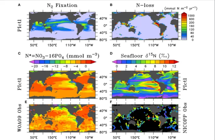
The patterns and rates of N2 fixation and N-loss are generally consistent with its observational biogeochemical indicators N∗and sedimentaryδ15N (Figure 2). Water column N-loss produces low N∗ and high δ15N in the ODZs of the eastern tropical Pacific and northern Indian Ocean.
FIGURE 2 | Preindustrial control (PIctl) annual vertically-integrated (A)N2fixation and(B)water column plus sedimentary N-loss. Comparison of upper ocean (0–300 m) N* and seafloorδ15N of PIctl(C,D)to(E)World Ocean Atlas 2009 (WOA09) (Garcia et al., 2010b) and(F)NICOPP database (Tesdal et al., 2013) observations.(B–D)Contours of minimum dissolved oxygen (10 mmol m−3) in the water column show where water column N-loss occurs.
Sedimentary N-loss delivers similar, but more moderate trends most notably on large continental shelves (e.g., Bering Sea, Patagonian Shelf). In the more oligotrophic tropics and subtropics, N2 fixation conversely generates high N∗ and low δ15N. Low NO−3 utilization due to iron limitation in HNLC regions of the Southern Ocean, North Pacific, and eastern equatorial Pacific drive low δ15N, whereas high utilization in the oligotrophic causes higher δ15N in the absence of N2
fixation.
Global mean δ15NO−3 is determined by global rates and isotope effects of N2fixation, and water column and sedimentary N-loss (Brandes and Devol, 2002; Altabet, 2007). Sedimentary N- loss rates and its isotope effect represent the largest uncertainties for determining global meanδ15NO−3 (Devries et al., 2013; Somes et al., 2013). Therefore, we took an empirical approach and chose the sedimentary N-loss fractionation factor (εSedNl = 6‰) within its estimated uncertainity range (1.5–13‰;Brandes and Devol, 1997; Lehmann et al., 2007; Granger et al., 2011;
Dale et al., 2014) that sets deep ocean δ15NO−3 near its observed ∼5‰ value given the model predicted rates of N2 fixation, water column N-loss, and sedimentary N-loss described above.
LAST GLACIAL MAXIMUM MODEL CONFIGURATIONS
Similar to Schmittner and Somes (2016) and guided by the Paleoclimate Model Intercomparison Project (PMIP3;Braconnot et al., 2012), we prescribe the LGM boundary conditions of the model: lower atmospheric concentrations of the greenhouse gases carbon dioxide, nitrous oxide, and methane, changes of Earth’s orbit, and the increased area and height of ice sheets (Peltier, 2004). The ocean grid bathymetry and total ocean volume remains unchanged relative to the preindustrial simulation. However, effects of reduced sea level on sedimentary N-loss are accounted for by calculating a new sub-grid scale bathymetry scheme assuming a constant 120 m sea level reduction (Figure S1). This is different from SS16, who neglected sea level effect. The marine biogeochemistry equations are identical in the preindustrial and LGM simulations with parameters given inTable 1.
Wind stress anomalies (LGM minus preindustrial) are prescribed using monthly averages of 8 models that participated in the PMIP3 (Muglia and Schmittner, 2015) since the UVic model does not include an atmospheric general circulation
TABLE 1 | Model configurations.
# Name Global euphotic
dissolved Fe (nmol m−3)
Global PO3−4 (mmol m−3)
RO:N ŴSedN−l
0 PIctl 0.192 2.17 10.6 2
1 LGMctl 0.251 2.50 (+15%) 10.6 2
2 LGMloFe 0.202 2.50 (+15%) 10.6 2
3 LGMhiFe 0.318 2.50 (+15%) 10.6 2
4 LGMloPO3−4 0.251 2.28 (+5%) 10.6 2
5 LGMhiPO3−4 0.251 2.71 (+25%) 10.6 2
6 LGMmidWCNl 0.251 2.50 (+15%) 11.0 2
7 LGMhiWCNl 0.251 2.50 (+15%) 11.4 2
8 LGMloSedNl 0.251 2.50 (+15%) 10.6 0.4
9 LGMhiSedNl 0.251 2.50 (+15%) 10.6 6
RO:Nis the oxygen to nitrogen stoichiometry for biogeochemical processes.ΓSedN−lis the sedimentary N-loss acceleration factor.
component (Figure S3). This is different from SS16, who used pre-industrial wind stress. As shown by Muglia and Schmittner (2015), LGM wind stress anomalies increase the Atlantic Meridional Overturning Circulation (AMOC). We further deviate from SS16 by reducing moisture diffusivity in the 2D energy-moisture balance atmospheric model across the Southern Ocean by a factor of 2. Reduced meridional atmospheric moisture flux has been suggested as an important mechanism to influence glacial stratification and carbon storage in the Southern Ocean (Sigman et al., 2007), which weakens and shoals the AMOC in our model. The resulting AMOC is weaker (∼9.9 Sv maximum) and shallower (by ∼500 m as indicated by shoaling of the zero streamfunction line in Figures 1B,E from ∼2,700 to ∼2,200 m), similar to that of SS16 due to the compensating effects of wind stress and moisture diffusivity changes. The simulations were initialized with results from SS16 and run for over 8,000 years as they approached their quasi steady-state solution.
Atmospheric Fe Deposition
We account for increased atmospheric Fe deposition during the LGM (Figure 3). LGM and preindustrial dust flux estimates were obtained fromAlbani et al. (2014). We assumed a 3.5% Fe content in dust, and variable solubility was used from an atmospheric model that simulates the relation between modern iron flux and solubility of iron in dust (Luo et al., 2008). We applied their relationship to LGM and preindustrial dust fluxes, thereby obtaining surface soluble atmospheric Fe fluxes (Figure S4).
To predict the surface soluble atmospheric Fe fluxes effect on dissolved Fe concentrations in our model, we analyzed the global relationship between soluble atmospheric Fe flux (atmFeflx) and dissolved Fe (dFe) in the upper ocean from a different model that includes Fe as a prognostic tracer (Nickelsen et al., 2015). The relationship that yielded the highest correlation (R=0.33) was a power law of the formdFe=A×(atmFeflx)BwhereA=6.3× 10⁻⁴andB=0.24 (Figure S4). LGM dissolved Fe was calculated asdFeLGM=(atmFeflxLGM/atmFeflxPI)B×dFePI. This pragmatic approach is used due to high uncertainties associated with
FIGURE 3 | Annual euphotic zone dissolved iron in (A)preindustrial control (PIctl) and the ratio relative to preindustrial of the LGM simulations(B) LGMloFe,(C)LGMctl, and(D)LGMhiFe based on LGM atmospheric deposition estimates (Albani et al., 2014).
atmospheric dust deposition rates and Fe solubility, responsible for soluble Fe deposition estimates that differ by over an order of magnitude in different preindustrial global marine iron models (Tagliabue et al., 2016). In our LGM Fe sensitivity experiments, we changed the exponentBby the value±0.2 from the LGM control value 0.25, which yields ± ∼20% changes to global euphotic zone dissolved Fe concentrations (Table 1, Figure 3).
PO
34−Inventory
We test a hypothesis that the global PO3−4 inventory was larger during the LGM mainly due to reduced organic phosphorus burial on the exposed continental shelves from lower sea level (Broecker, 1982; Wallmann, 2010; Wallmann et al., 2016). Since the global oceanic PO34− inventory is conserved in each model simulation, we implement this hypothesis by imposing the estimated+ ∼15% increase in the global PO3−4 inventory from
Wallmann et al. (2016)in LGMctl (Table 1). Model experiments
#4 LGMloPO34− and #5 LGMhiPO34− probe its sensitivity to
±10% global PO34−change relative to LGMctl.
N-Loss Rates
We perform additional simulations to investigate how different water column and sedimentary N-loss rates affect LGM nitrogen cycling andδ15N distributions. In the model, water column N- loss can be increased pragmatically by increasing the elemental ratio of oxygen consumed per organic nitrogen remineralized (RO:N, see Table 1). This leads to more oxygen loss, lower oxygen concentrations and larger ODZs in the model, thereby increasing water column N-loss. We interpret these simulations as water column N-loss sensitivity experiments rather than predictions of higher RO:N stoichiometry, however noting that Devries and Deutsch (2014) suggest this ratio is higher in more stratified, nutrient depleted surface regimes that are more prevalent features in the LGM. Model experiment #6 (LGMmidWCNl) and #7 (LGMhiWCNl) assume RO:N ratios of 11.0 and 11.4, respectively, compared to the standard value of 10.6 used in the preindustrial and LGM control simulations.
Sedimentary N-loss has been altered separately by changing its rate only on the subgrid-scale bathymetry scheme. We have applied an acceleration parameterization focused on narrow continental shelves in the upper 250 m to account for poorly resolved coastal processes (e.g., upwelling) that fuel sedimentary N-loss there (Figure S1). In the control simulations, applying an acceleration factor of 2 in this scheme increases sedimentary N-loss by 29 Tg N yr-1 (44%) in PIctl and 11 Tg N yr−1 (29%) in LGMctl. LGM model experiments #8 LGMloSedNl and #9 LGMhiSedNl demonstrate the model sensitivity to this parameterization with lower and higher factors (Table 1), respectively, which altered global rates by ± ∼40% relative to LGMctl (Table 2) in this sensitivity test. Note that since LGMloSedNl does not contain the sedimentary N-loss acceleration formulation, its factor is applied directly to the sedimentary N-loss rate on the subgrid-scale scheme. These N-loss sensitivity simulations were
initialized with LGMctl and run for an additional 4,000 years.
LGM MODEL RESULTS
In this section, we first provide a brief overview of the physical climate since the focus of this study is on marine biogeochemistry, noting that the physical climate (e.g., temperature and circulation) is identical for all LGM simulations. The subsequent subsection describes the LGMctl biogeochemistry relative to PIctl, followed by the LGM sensitivity experiments.
Physical Climate
The model reproduces major physical characteristics of the LGM climate, which are identical in all LGM simulations. Global average surface air temperature is 4.3◦C colder in the LGMctl.
The AMOC is shallower and weaker (9.9 Sv) compared to PIctl (17.1 Sv; Figure 1). Global mean 114C values are −165 and
−225‰ in PIctl and LGMctl, respectively. Bottom waters in the LGMctl simulation are colder everywhere and saltier except for the eastern North Atlantic, where they are fresher compared with PIctl (Figure S5) due to the shoaling and weakening of the AMOC since Antarctic Bottom Water is fresher than North Atlantic Deep Water in the model. The simulated pattern of salinity changes indicates enhanced brine rejection from intensified sea ice formation in the Weddell Sea. The basin scale simulated changes in bottom water properties are qualitatively consistent with observations (Figure S5;Adkins et al., 2002; Insua et al., 2014). The simulated decrease of 114C below 2 km depth (−75‰, ∼800 years radiocarbon age) is slightly older than a recent estimate of∼600 years based on sediment reconstructions (Sarnthein et al., 2013).
LGM Control Marine Biogeochemistry
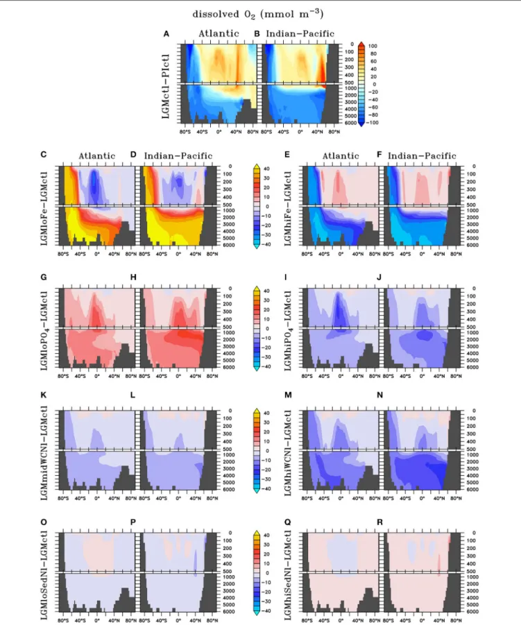
In LGMctl, oxygen concentrations are higher above∼1,500 m and lower below (Figures 4A,B) relative to PIctl, which is consistent with O2reconstructions (Jaccard and Galbraith, 2012).
The colder LGM climate enhances sea surface solubility of oxygen that is responsible for the upper ocean increase (Meissner et al.,
TABLE 2 | Global biogeochemical model results.
# Name NPP EXP O2 ODZ volume NO−3 δ15NO−3 N2fixation WC N-loss Sed. N-loss
(Gt C yr−1) (Gt C yr−1) (mmol m−3) (x1014m3) (mmol m−3) (‰) (Tg N yr−1) (Tg N yr−1) (Tg N yr−1)
0 PIctl 48.7 7.2 187 23.0 30.9 5.45 159 68.0 90.9
1 LGMctl 33.0 6.4 150 12.1 37.7 5.64 65.0 14.8 49.6
2 LGMloFe 36.8 6.4 173 9.1 37.4 5.67 76.1 25.2 49.1
3 LGMhiFe 30.5 6.3 131 57.8 36.6 6.13 68.5 19.9 48.7
4 LGMloPO3−4 29.5 5.9 162 0.027 34.9 5.02 46.5 2.1 44.0
5 LGMhiPO3−4 36.3 6.9 139 68.8 39.0 6.50 98.2 43.0 54.4
6 LGMmidWCNl 32.7 6.3 143 41.5 36.8 6.35 77.2 26.5 49.6
7 LGMhiWCNl 32.2 6.3 136 78.0 35.3 7.04 94.6 42.2 49.3
8 LGMloSedNl 33.2 6.4 148 24.3 38.5 5.77 50.2 19.1 27.9
9 LGMhiSedNl 32.9 6.3 151 6.4 37.1 5.25 79.2 10.9 68.4
FIGURE 4 | Zonal dissolved oxygen differences in the Atlantic and Indian-Pacific Oceans, respectively, of (A,B)Last glacial Maximum control (LGMctl) minus preindustrial control (PIctl) and the Last Glacial Maximum simulations minus LGM control:(C,D)LGMloFe,(E,F)LGMhiFe,(G,H)LGMloPO3−4 ,(I,J) LGMhiPO3−4 ,(K,L)LGMmidWCNl,(M,N)LGMhiWCNl,(O,P)LGMloSedNl, and(Q,R)LGMhiSedNl.
FIGURE 5 | Vertically-integrated differences of N2fixation and total N-loss, respectively, of (A,B)Last Glacial Maximum control (LGMctl) minus preindustrial control (PIctl) and the Last Glacial Maximum simulations minus LGM control:(C,D)LGMloFe,(E,F)LGMhiFe,(G,H)LGMloPO3−4 ,(I,J)LGMhiPO3−4 ,(K,L)
LGMmidWCNl,(M,N)LGMhiWCNl,(O,P)LGMloSedNl, and(Q,R)LGMhiSedNl. Contours of minimum dissolved oxygen (10 mmol m−3) in the water column show where water column N-loss occurs.
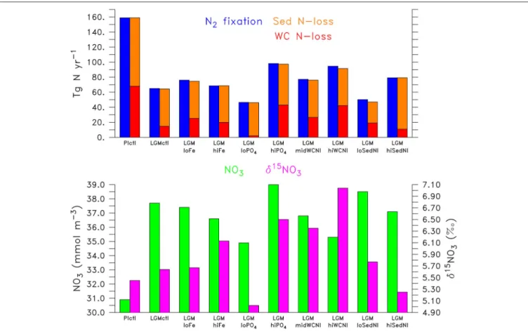
FIGURE 6 | (Top)Global N2fixation (left blue bar), water column N-loss (right red bar), and sedimentary N-loss (right orange bar) for the simulations.(Bottom)Global NO−3(left green bar) and globalδ15NO−3 (right magenta bar) for the simulations.
2005). The combination of the more sluggish AMOC (Figure 1C) and increased sea ice cover, which reduce oxygen supply to the deep ocean, and enhanced atmospheric Fe deposition (Figure 3), which fuels organic matter export production that increases subsurface oxygen consumption, are the main factors responsible for the decreased deep ocean oxygen concentrations. On the global average, there is a 21.5% reduction of the global O2
inventory (Table 2). This is similar to the 20.8% reduction resulting from SS16’s bestδ15N simulation, who attribute∼7% of this decrease to physics and∼14% to changes in Fe fertilization.
Higher O2 concentrations in the upper ocean reduce the volume of ODZs by 47% and water column N-loss by 78%
(Figures 5B,6). The difference in the reduction of ODZ volume compared to water column N-loss rate occurs due to the emergence of a ODZ in the deep (1,000–2,000 m) subarctic Pacific that accounts for 10% of total water column N-loss in LGMctl, which cannot be excluded because trace metal proxies at bottom waters in these locations indicate less oxygen during the LGM (Jaccard and Galbraith, 2012). Here, OM remineralization rates that drive water column N-loss are lower than in the shallower tropical ocean, which results in less water column N-loss per volume of ODZ waters. In combination with decreased sedimentary N-loss by 55% due to exposed continental shelves from lower sea level in LGMctl (e.g., Bering
Sea Shelf, North Atlantic;Figure 5B), total N-loss decreases by 59% (Table 2, Figure 6). However, note that some regions at mid-latitudes in the Southern Ocean, North Pacific, and North Atlantic show increases in sedimentary N-loss due enhanced atmospheric Fe deposition fueling additional export production (Figure 5B). Although reduced total N-loss occurs primarily in the upper ocean, the resulting increased NO−3 accumulates in the deep ocean due to enhanced POM export in the Southern Ocean that remineralizes and remains for longer in the older, more sluggish Antarctic Bottom Waters in LGMctl.
N2 fixation decreases in the LGMctl simulation by 59%
mainly in response to the reduction in N-loss when approaching the steady-state solution (Figures 5, 6). Only the oligotrophic eastern tropical Pacific and southern boundary of the southern subtropical gyres show subtle increases of N2 fixation due to enhanced atmospheric Fe deposition (Figure 5A). In the LGMctl model, global N2fixation is not sensitive to increased Fe deposition because glacial estimates of increased Fe deposition applied here (Albani et al., 2014) primarily occur at high latitudes where diazotrophs are limited by temperature. However, the combined effects of the changes in sources and sinks result in a significantly increased global NO−3 inventory (+22%). Note that DOP utilization by diazotrophs does not play a significant role stimulating N2 fixation in LGMctl because nitrogen limitation
is reduced due to the larger NO−3 inventory and thus ordinary phytoplankton outcompete diazotrophs for the majority of DOP consumption.
Atmospheric Fe Deposition Sensitivity
Atmospheric Fe deposition was increased during the LGM compared to pre-industrial times, which has a large fertilizing effect on organic matter production in the HNLC regions of the Southern Ocean, subarctic North Pacific, and equatorial eastern Pacific in the model. Additional NO−3 is thus consumed at the surface and stored in the deep ocean (Figures 7A,B), where it can remain for millennia.
Enhanced export production at high latitudes reduces the amount of preformed surface NO−3 in Subantarctic Mode Waters that flow to the tropics (Figures 7C–F). This reduces tropical productivity, volume of tropical ODZs and global water column N-loss in LGMhiFe relative to LGMloFe (Table 2). Intermediate waters (∼1,000–2,000 m) in the subarctic North Pacific are near the threshold of suboxia in simulation LGMctl. Those suboxic regions intensify when enhanced atmospheric Fe deposition in LGMhiFe stimulates additional organic matter remineralization (Figure 4F), which enhances water column N-loss (Figure 5F).
Only minor increases to N2 fixation are stimulated by enhanced atmospheric Fe deposition in the model (Figure 5E).
This is most pronounced in two zones in the southern hemisphere that are largely Fe limited in the preindustrial ocean:
the eastern tropical Pacific and a zonal band across the edge of the southern subtropical gyres. Since diazotrophs prefer warm oligotrophic N-limited surface conditions, they grow outside the cold, high surface NO−3 waters of the eastern equatorial Pacific upwelling region. Although, not typically thought to occur outside the tropics, the strong atmospheric Fe deposition originating around Patagonia (Figure 3) is sufficient to stimulate N2fixation in our model. However, on the global average, these areas of additional N2 fixation are much smaller than areas in which N2 fixation decreased in model LGMctl relative to PIctl due to reduced N-loss (Figure 5A).
Water column δ15NO−3 is strongly influenced by nitrogen cycling changes in response to enhanced atmospheric Fe deposition (Figure 8). Enhanced (reduced) surface NO−3 utilization increases (decreases) surfaceδ15NO−3 in the Southern Ocean and Subarctic Pacific in LGMhiFe (LGMloFe). The minor increase (decrease) to N2 fixation rates in the southern tropics and subtropics in LGMhiFe (LGMloFe) substantially decreases (increases) δ15NO−3. This large isotopic signal occurs because these systems switch from being driven by high NO−3 utilization, which causes extremely 15N-enriched surface NO−3, to a N2
fixation isotopic regime that introduces 15N-depleted nitrogen to the surface ocean. This model prediction suggests that all relevant processes should be considered when interpreting δ15N and the change to the isotopic signal may not be linearly representative of the rate change to one specific nitrogen cycling process alone.
Global PO3−4 Inventory Sensitivity
The model simulations testing a hypothesized increase to the global PO3−4 inventory predict larger NO−3 inventories due
to enhanced N2 fixation (Table 2, Figures 6, 7G–J). PO34− is the major limiting macronutrient for N2-fixing diazotrophs.
Although N-loss is reduced during the LGM, N-limitation still persists, leaving the tropical and subtropical ocean mostly N limited. Therefore, increased PO34−stimulates additional growth of diazotrophs via N2 fixation that is most pronounced in the tropical ocean. The additional organic matter production via enhanced N2 fixation and remineralization at depth stimulates additional water column N-loss, which balances the enhanced N2
fixation at a new steady-state with a larger global NO−3 (Figure 6) and reduced O2inventory (Figures 4I,J). A 10% increase in the PO34−inventory thus causes an 8% increase in the NO−3 inventory (LGMctl-LGMloPO34−). However, a further 10% increase in the PO3−4 inventory (LGMhiPO3−4 -LGMctl) leads to diminishing returns in terms of NO−3 (4%) due to the further expansion of ODZs and N-loss. The additional N2 fixation decreases surface δ15NO−3 in the tropics and subtropics, whereas the additional water column N-loss increases subsurfaceδ15NO−3 in the Indian and Pacific (Figures 8I,J).
N-Loss Sensitivity
The water column N-loss sensitivity simulations alter rates by increasing oxygen consumption during organic matter remineralization, thereby decreasing subsurface oxygen concentrations (Figures 4K–N). Note that these simulations do not change the large-scale pattern of higher oxygen in the upper ocean and lower oxygen in the deep ocean that is supported by observational constraints (Jaccard and Galbraith, 2012), but only reduces the magnitude of this qualitative trend in the deep ocean. Enhanced water column N-loss in the expanded ODZs in LGMmidWCNl and LGMhiWCNl reduces NO−3 in the eastern tropical Pacific, North Indian, and subarctic Pacific (Figures 7K–N).
This significantly increases subsurface δ15NO−3 since water column N-loss has a strong isotope effect (Figures 8K–N).
Even though this signal is generated in the ODZs of the tropical ocean and subarctic Pacific, it eventually reaches the Southern Ocean and has a global impact (Figures 8K–N).
Sedimentary N-loss has lower local rates that are spread throughout all ocean basins so its signal is more distributed through the global ocean compared to vertically-integrated water column N-loss. Enhanced (reduced) rates in LGMhiSedNl (LGMloSedNl) decreases (increases) global NO−3 (Figures 7O–R). Since sedimentary N-loss has a relatively small isotope effect, its main isotopic signal is an indirect one by stimulating additional (less) N2fixation to balance additional (less) sedimentary N-loss in LGMhiSedNl (LGMloSedNl).
This decreases (increases) surfaceδ15NO−3 most notably in the tropical and subtropical ocean basins (Figures 8O–R).
NITROGEN ISOTOPE MODEL-DATA ANALYSIS
Modeled nitrogen isotopes are compared to 61 datapoints from the recent synthesis of reconstructions from the Nitrogen Cycling
FIGURE 7 | Zonal dissolved nitrate (NO−3) differences in the Atlantic and Indian-Pacific Oceans, respectively, of (A,B)Last glacial Maximum control (LGMctl) minus preindustrial control (PIctl) and the Last Glacial Maximum simulations minus LGM control:(C,D)LGMloFe,(E,F)LGMhiFe,(G,H)LGMloPO3−4 ,(I,J) LGMhiPO3−4 ,(K,L)LGMmidWCNl,(M,N)LGMhiWCNl,(O,P)LGMloSedNl, and(Q,R)LGMhiSedNl.
FIGURE 8 | Zonal dissolvedδ15N of nitrate (δ15NO−3) differences in the Atlantic and Indian-Pacific Oceans, respectively, of (A,B)Last glacial Maximum control (LGMctl) minus preindustrial control (PIctl) and the Last Glacial Maximum simulations minus LGM control:(C,D)LGMloFe,(E,F)LGMhiFe,(G,H)LGMloPO3−4 , (I,J)LGMhiPO3−4 ,(K,L)LGMmidWCNl,(M,N)LGMhiWCNl,(O,P)LGMloSedNl, and(Q,R)LGMhiSedNl.
in the Oceans Past and Present (NICOPP) group (Galbraith et al., 2013) for which LGM—Late Holocene differences are available.
These data, based on bulk organic nitrogen measurements, were corrected for a diagenetic effect according to Robinson et al.
(2012), who examined over 100 locations and found a significant correlation with water depth (∼1‰/km), while noting that oxygen exposure time is likely the main driver. We use the five additional foraminifera and diatom bound measurements included in Schmittner and Somes (2016), plus 6 more from recent studies in the subarctic Pacific and central equatorial Pacific (Ren et al., 2015; Costa et al., 2016), all of which were not corrected for diagenesis. Although combining different forms ofδ15N records creates uncertainty, excluding the diatom and foraminifera bound measurements does not affect which simulations performed best in terms of the statistical model-data metrics so we include them into the main analysis to improve spatial coverage.
Overall,δ15N records from LGM sediments document lower values in modern ODZs such as the eastern tropical Pacific and Arabian Sea indicating less water column N-loss, higher values in the western tropics of the North Pacific and North Atlantic indicating less N2 fixation, and higher values in high latitude HNLC regions (i.e., Southern Ocean, western subarctic Pacific) indicating enhanced surface NO−3 utilization (Figures 9–11).
These sedimentaryδ15N records are compared to theδ15N values of sinking particulate organic nitrogen (PON) in bottom waters above the seafloor, which we refer to as sedimentaryδ15N in the model below. Our model does not account for terrestrial sources ofδ15N, which can influence records near the continental margin and potentially contribute to model-data misfits. Therefore, we focus our analysis and discussion on regions that are strongly influenced by marine nitrogen cycling processes, but note that all data points are included in the model-data statistical metrics.
LGM Control Simulation
Model simulation LGMctl, which includes enhanced atmospheric Fe deposition and assumes a +15% increase to the global PO34− inventory, reproduces the major trends in the LGM reconstructions (R=0.45,Table 3;Figures 9–11). It reproduces the largest increase in δ15N in the Southern Ocean with respect to preindustrial values (Figure 11B) and the smaller increase in the subarctic Pacific HNLC region (Figure 11F).
However, it predicts a slight increase (+0.7‰) to the Central Equatorial Pacific, where the data show a minor decrease (−0.2‰). The largest model-data mismatch exists in the Eastern Tropical North Pacific ODZ, where the predicted decrease of δ15N is too strong relative to observations (Figure 11C).
The change to globalδ15NO−3 (Table 2) and sedimentaryδ15N (Figure 11A) in LGMctl relative to PIctl is small compared to the change of the ratio of sedimentary to water column N-loss, which in part determines global δ15NO−3 (Somes et al., 2013).
This relatively smallδ15NO−3 change is due to the dilution effect in N-loss zones (Deutsch et al., 2004), which increases the isotope effect of water column N-loss (per mole N removed) in LGMctl relative to PIctl as NO−3 utilization decreases in the smaller ODZs.
This effect decreases the isotopic signature ofδ15N removed by
water column N-loss from−5.1‰ in PIctl to−10.3‰ in LGMctl, thereby increasing its isotope effect by 5.2‰. This also occurs to a lesser degree in bottom waters where sedimentary N-loss occurs increasing its isotope effect by 1.1‰. Therefore, additional N2
fixation and thus a higher ratio of sedimentary to water column N-loss is required to balance the increased isotope effect from N-loss on globalδ15NO−3 in the LGMctl steady-state solution compared to PIctl.
The processes that lead to slightly higher deep oceanδ15NO−3 in LGMctl are mainly controlled at high latitudes. In the North Atlantic, reduced N2 fixation elevates surface δ15NO−3 that eventually subducts in the Atlantic meridional overturning circulation and increases deep ocean δ15NO−3 (Figure 8A).
In the Southern Ocean, enhanced atmospheric Fe deposition increases NO−3 utilization and the isotopic signature of sinking particulate organic nitrogen (PON) that remineralizes at depth (Figures 8A,B,9B). The emergence of a small ODZ in the deep (1,000–2,000 m) subarctic Pacific (Figure 5B), which accounts for 10% of total water column N-loss in LGMctl, contributes to elevated deep oceanδ15NO−3 as well. Since most of the increased NO−3 inventory in LGMctl accumulates in these old, sluggish deep waters, our modeling suggests that high latitude process also play a role determining global meanδ15NO−3, not only N2
fixation and water column N-loss in the tropics.
Atmospheric Fe Deposition Sensitivity
Lower atmospheric Fe deposition in LGMloFe compared to LGMctl reduces NO−3 utilization and sedimentary δ15N in HNLC regions (Figures 9C,D), where the fit with observations deteriorates (Figures 10B,11B). The better agreement of the magnitude of the increase inδ15N in LGMctl in the Southern Ocean and Subarctic Pacific supports LGMctl’s assumption for increased Fe deposition during the LGM in those regions. In fact, LGMctl’s increase in NO−3 utilization may be underestimated in the Southern Ocean, where simulation LGMhiFe agrees better with the observations (Figure 11B).
In the Central Equatorial Pacific, which is on the western border of the eastern Pacific HNLC region, both LGM Fe sensitivity simulations reproduce the observations better than LGMctl (Figure 11D), but for different reasons. In LGMloFe, the small increase to atmospheric Fe deposition was insufficient to increase NO−3 utilization and hence sedimentary δ15N in this region. In our high-end simulation for atmospheric Fe deposition (LGMhiFe), enhanced N2 fixation introducing additional15N- depleted nitrogen reduces the overestimated model bias of LGMctl. Until more observations in and around the central and eastern tropical Pacific HNLC become available, it will remain difficult to evaluate whether relatively low NO−3 utilization or increased N2fixation was the most important process driving the observed decreased LGMδ15N trend.
Our sensitivity model experiments in the Southern Hemisphere show a balance between lower δ15N due to enhanced N2 fixation in the subtropics and higher δ15N from enhanced surface NO−3 utilization toward high latitudes. Our model predicts that increased Fe could stimulate additional N2 fixation at the poleward edge of the southern subtropics as far south as ∼40◦S, which counteracts with the isotope
FIGURE 9 | Sedimentaryδ15N of (A)LGM minus preindustrial observations and(B)Last Glacial Maximum control (LGMctl) minus preindustrial control (PIctl).
Sedimentaryδ15N differences of the Last Glacial Maximum simulations:(C,D)LGMloFe,(E,F)LGMhiFe,(G,H)LGMloPO3−4 ,(I,J)LGMhiPO3−4 ,(K,L)LGMmidWCNl, (M,N)LGMhiWCNl,(O,P)LGMloSedNl, and(Q,R)LGMhiSedNl minus PIctl and minus LGMctl are shown, respectively.
FIGURE 10 | Comparison of LGM minus PI changes in sedimentaryδ15N from observations (horizontal axis) and model results (vertical axis) of (A) LGMctl,(B)LGMloFe,(C)LGMloPO3−4 ,(D)LGMhiFe,(E)LGMhiPO3−4 ,(F)LGMmidWCNl,(G)LGMloSedNl,(H)LGMhiWCNl, and(I)LGMhiSedNl. Locations in the Pacific, Atlantic, and Indian Oceans are shown as circles, squares, and triangles, respectively. Locations in oxygen deficient zones (ODZ; minimum O2<
10 mmol m−3) are shown as blue crosses and Southern Ocean (south of 40◦S) are red Xs. The black line indicates a “perfect” representation of observations.
effect of enhanced NO−3 utilization that increases δ15N at higher latitudes (Figures 8C–F, 9C–F). As NO−3 decreases with enhanced atmospheric Fe deposition, the additional
15N-depleted nitrogen via N2 fixation contributes to a larger fraction of total sinking PON, which prevents a higher
δ15N increase in LGMhiFe compared to the δ15N decrease in LGMloFe (Figure 11B). The absence of open ocean δ15N observations in the tropical and subtropical southern hemisphere makes it uncertain to validate this increase to N2 fixation there.
FIGURE 11 | Regional Last Glacial Maximum minus Preindustrialδ15N differences of LGM model simulations (#1) LGMctl, (#2) LGMloFe, (#3) LGMhiFe, (#4) LGMloPO3−4 , (#5) LGMhiPO3−4 , (#6) LGMmidWCNl, (#7) LGMhiWCNl, (#8) LGMloSedNl, (#9) LGMhiSedNl in the (A)global ocean,(B)Southern Ocean (<40◦S),(C)oxygen deficient zones (minimum O2<10 mmol m−3),(D)Central Equatorial Pacific (170◦W–130◦W, 5◦N–5◦S),(E)Western Tropical North Atlantic and Pacific (0–25◦N, western 50◦of Atlantic and Pacific basins), and(F)Subarctic Pacific (40–65◦N). “Data-masked” model (dark blue left bar) only includes locations where data exist, whereas the “full” model (light blue right bar) averages over the entire region.
TABLE 3 |δ15N model-data statistical metrics.
# Name R STD RMS error Global bias
0 PIctl 0.53 1.13 1.09 +0.64
1 LGMctl 0.45 1.69 1.54 −0.29
2 LGMloFe 0.27 1.41 1.54 −0.56
3 LGMhiFe 0.48 1.97 1.73 −0.21
4 LGMloPO3−4 0.50 1.90 1.81 −1.03
5 LGMhiPO3−4 0.40 1.70 1.60 +0.22
6 LGMmidWCNl 0.43 1.67 1.54 +0.19
7 LGMhiWCNl 0.41 1.79 1.68 +0.42
8 LGMloSedNl 0.45 1.68 1.54 +0.36
9 LGMhiSedNl 0.45 1.73 1.66 −0.90
Correlation coefficient (R), standard deviation (STD), and root-mean squared error (RMS error) and global average bias of the model-data analysis after observations were interpolated onto the model grid. STD and RMS error are normalized by the standard deviation of observations. LGM simulation metrics are calculated as changes relative to PI (i.e., LGM−PI), whereas for PIctl the absolute values shown inFigures 2D,Fare used.
Global PO
34−Inventory Sensitivity
In the model, a larger global PO34−inventory stimulates increases to N2 fixation, water column N-loss, and the global NO−3
inventory (Figure 6). This results in increased sedimentary δ15N near ODZs and decreased δ15N outside of them in the more oligotrophic ocean where additional N2 fixation occurs (Figure 9J). The magnitude of change to δ15N in the model (Figure 10) is relatively small because N2 fixation and water column N-loss have counteracting nitrogen isotopic effects. Since these processes occur within close spatial proximity in the tropics, the input of15N-depleted nitrogen via fixation roughly compensates the extra15N-enriched NO−3 via enhanced water column N-loss rates, preventing a larger change to the large scale δ15N signal (Figures 9G–J).
Despite large changes to the global rates of these processes, changes to simulated δ15N at the location of observations only moderately affect the model-data statistical metrics (Table 3, Figure 10). The higher water column N-loss in LGMhiPO3−4 better reproduces δ15N in tropical ODZs (Figure 11C). However, the additional water column N-loss in the subarctic Pacific overestimates δ15N in that region. The model experiment LGMloPO34− performs best in the Central Equatorial Pacific (Figure 11E), which suggests that the additional PO3−4 stimulates too much N2 fixation there in simulations LGMctl and LGMhiPO3−4 .