During the Last Glacial Maximum

(1)

During the Last Glacial Maximum

Zhaoyang Song¹ , Mojib Latif^1,2 , and Wonsun Park¹

1GEOMAR Helmholtz Centre for Ocean Research Kiel, Kiel, Germany,²Excellence Cluster“The Future Ocean”, Kiel University, Kiel, Germany

Abstract

The variability of the Atlantic meridional overturning circulation (AMOC) and its governing processes during the Last Glacial Maximum (LGM) is investigated in the Kiel Climate Model. Under LGM conditions, multidecadal AMOC variability is mainly forced by the surface heatﬂux variability linked to the East Atlantic pattern (EAP). In contrast, the multidecadal AMOC variability under preindustrial conditions is mainly driven by the surface heatﬂux variability associated with the North Atlantic Oscillation.

Stand‐alone atmosphere model experiments show that relative to preindustrial conditions, the change in AMOC forcing under LGM conditions is tightly linked to the differences in topography.

Plain Language Summary

The Last Glacial Maximum (LGM, about 21,000 years before present) was a period when extensive continental ice sheets covered parts of North America and northern Europe. A climate model simulates enhanced multidecadal variability of the Atlantic meridional overturning circulation (AMOC), a major oceanic current system with global climatic impacts, during the LGM relative to modern times. The main driver of multidecadal AMOC variability under LGM conditions is the surface heatﬂux variability associated with the East Atlantic pattern, a mode of internal atmospheric variability.

Under modern conditions, the main driver of the multidecadal AMOC variability is the heatﬂux variability associated with the North Atlantic Oscillation, another mode of internal atmospheric variability. The difference in AMOC forcing is basically due to the change in topography linked to the extensive ice sheets during the LGM.

1. Introduction

During the Last Glacial Maximum (LGM) about 21,000 years before present, global ice volume reached its maximum (Mix et al., 2001). Concurrent with expanded Antarctic and Greenland ice sheets, there were extensive continental ice sheets over parts of North America and northern Europe during that time.

Coupled climate models and atmosphere models have shown that the ice sheets, along with much lower concentrations of atmospheric greenhouse gases (e.g., Bereiter et al., 2015), force large perturbations in the mean atmospheric circulation and its internal variability over the North Atlantic sector, especially during boreal winter (e.g., Justino & Peltier, 2005; Pausata et al., 2009; Pausata et al., 2011). There are two prominent modes of internal atmospheric variability over this region: the North Atlantic Oscillation (NAO) and the East Atlantic pattern (EAP). The NAO is the leading mode of atmospheric circulation variability over the North Atlantic/European sector in boreal winter, characterized by a meridional dipole structure with a low‐pressure center over Iceland and high‐pressure center over the Azores (e.g., Hurrell, 1995). The second most energetic mode is the EAP. The EAP is structurally similar to the NAO and consists of a north‐south dipole, with the anomaly centers of the EAP located southeastward to the approximate nodal lines of the NAO pattern (Barnston & Livezey, 1987). The NAO and EAP drive climate variations via anomalous surface winds and heatﬂuxes (Cayan, 1992).

The North Atlantic Ocean plays a crucial role in the global climate system through a basin‐wide thermohaline circulation, the Atlantic meridional overturning circulation (AMOC), which is driven by deep water formation at high northern latitudes. The AMOC is characterized by the northwardﬂow of upper‐layer warm waters by the Gulf Stream and its extensions and its southward returnﬂow of cold waters by the deep western boundary current. The AMOC exhibits variability on a wide range of time scales, from monthly to centennial (Balan et al., 2011; Danabasoglu et al., 2016; Kanzow et al., 2010; Medhaug et al., 2012; Menary et al.,

This is an open access article under the terms of the Creative Commons Attribution License, which permits use, distribution and reproduction in any medium, provided the original work is properly cited.

Key Points:

• Multidecadal AMOC variability during the LGM and its associated physical processes have been investigated by means of a climate model

• Multidecadal AMOC variability during the LGM is mainly driven by surface heatﬂux variability linked to the East Atlantic pattern as opposed to the North Atlantic Oscillation under preindustrial conditions

• Change in topography during the LGM is responsible for the change in AMOC forcing

Supporting Information:

•Supporting Information S1

Correspondence to:

Z. Song, zsong@geomar.de

Citation:

Song, Z., Latif, M., & Park, W. (2019).

East Atlantic pattern drives multidecadal Atlantic meridional overturning circulation variability during the Last Glacial Maximum.

Geophysical Research Letters,46, 10,865–10,873. https://doi.org/10.1029/

2019GL082960

Received 22 MAR 2019 Accepted 5 SEP 2019

Accepted article online 11 SEP 2019 Published online 10 OCT 2019

(2)

2012). Climate models suggest that variations of the AMOC, through associated variations in northward heat transport, have the potential to drive surface climate variability, especially over the North Atlantic sector and on decadal to multidecadal time scales. AMOC impacts have been documented with respect to northeast Brazil and Sahel rainfall (Folland et al., 1986, 2001), Atlantic hurricanes (Wang & Lee, 2009), and summer climate over North America and Western Europe (Sutton &

Hodson, 2005).

Climate models simulate pronounced multidecadal AMOC variability throughout the last millennium and the Holocene (Wei & Lohmann, 2012; Zanchettin et al., 2013). In many climate models (Danabasoglu et al., 2012; Delworth et al., 2016; Kim et al., 2018), the multidecadal AMOC variability under present‐day conditions is strongly linked to NAO‐related changes in surface heat ﬂux over the subpolar North Atlantic. A few modeling studies suggest that the multidecadal AMOC variability could be also closely related to the EAP (Msadek & Frankignoul, 2009; Ruprich‐Robert & Cassou, 2015).

However, the multidecadal AMOC variability during the LGM and its governing physical processes so far only have received little attention. Under the LGM boundary conditions, large perturbations in mean atmospheric circulation and its internal variability, massively extended sea ice and shifted deep convection sites over the North Atlantic Sector are simulated by climate models. These changes can essentially affect the response of subpolar North Atlantic deep convection to the atmospheric forcing and subsequently the AMOC. A major goal of this study is to identify possible differences in the multidecadal AMOC variability between the LGM and modern times. In particular, we are interested in the atmospheric forcing of multidecadal AMOC variability.

Here we use the Kiel Climate Model (KCM; Park et al., 2009) to investigate the multidecadal AMOC variability during the LGM and compare it to that simulated under preindustrial conditions. The paper is orga- nized as follows: Section 2 describes the climate model and the experimental setup. In section 3, the multidecadal AMOC variability simulated under LGM conditions and its driving factors are explored.

Summary and discussion are presented in section 4 and conclude the paper.

2. Model, Experimental Setup, and Method

The KCM (Park et al., 2009) is a fully coupled atmosphere‐ocean‐sea ice general circulation model. In the version applied here, the atmospheric component ECHAM5 (Roeckner et al., 2003) is used with a horizontal resolution of T42 (2.8° × 2.8°) and 19 vertical levels reaching up to 10 hPa. The ocean‐sea ice component NEMO (Madec, 2008) is run on a 2° Mercator mesh and with 31 vertical levels. Enhanced meridional resolution of 0.5° is used in the equatorial region. The two models are coupled with the OASIS3 coupler (Valcke, 2006).

Two simulations are performed: one 5,300‐year‐long preindustrial control run (PI) that is initialized with the Levitus climatology of temperature and salinity. PI employs the modern land‐sea mask, orography, and continental ice sheet conﬁguration. In the other simulation for the glacial period (GLAC), the boundary conditions are implemented in accordance with the Paleoclimate Modelling Intercomparison Project phase 4 (PMIP4) protocol for LGM experiments (Kageyama et al., 2017). The ice sheet conﬁguration is an average of three different reconstructions following the PMIP3 LGM experiments (Braconnot et al., 2012). The greenhouse gas concentrations and orbital parameters are listed in Table 1. To account for the 116‐m drop of the mean sea level, GLAC is initialized with the Levitus temperature climatology and Levitus salinity climatology to which 1 psu has been added. GLAC is integrated for 4,650 years to reach quasi‐equilibrium (Figure 1a).

Monthly output from the last 1,000 years of the two integrations is used for analysis.

To extract the dominant modes of atmosphere‐ocean variability over the North Atlantic, widely used empirical orthogonal functions (EOFs) analysis is applied here (Chapter 13.5 in Jolliffe, 2002). EOF analysis decom- poses a multivariate data set into eigenvectors (EOFs) for spatial structure. The time evolution of each EOF, the principal components (PCs), are obtained by projection of the original data on the corresponding EOF.

The EOFs are orthogonal and sorted by the amount of explained variance in a descending order.

Table 1

Overview of Experimental Setup

Greenhouse gases & Orbital parameters PI GLAC

CO₂ 286 ppm 190 ppm

N₂O 805 ppb 375 ppb

CH₄ 276 ppb 200 ppb

Eccentricity 0.016724 0.018994

Obliquity 23.446° 22.949°

Perihelion 282.9° 294.42°

Note. The units ppm and ppb refer to parts per million and parts per bil- lion, respectively.

10.1029/2019GL082960

Geophysical Research Letters

(3)

3. Results

3.1. Mean State and AMOC

The JFM (January‐February‐March) sea surface temperature (SST) averaged over the North Atlantic (40–60°N) in PI and GLAC are 7.3 °C and 3.0 °C, respectively (Figures 1b and 1c). The colder SSTs in GLAC favor a substantial increase of sea ice extent. In PI, sea ice covers the Baffin Bay, the Labrador Sea, and western Greenland‐Iceland‐Norwegian (GIN) Sea (contours in Figures 1d and 1e). Deep convection (as indicated by JFM mixed layer depth) in PI is simulated basically east of the sea ice margin. In GLAC, one rather large deep convection site is simulated in the eastern North Atlantic south of Iceland (color shading in Figures 1d and 1e). There is a stronger low sea level pressure (SLP) center over the North Atlantic in GLAC relative to PI (Figures 1f and 1g), which goes along with enhanced negative surface heatfluxes (i.e., oceanic heat loss) over the convection site in the eastern North Atlantic (Figures 1h and 1i). The enhanced oceanic heat loss in GLAC is likely due to the intensified north‐easterlies implied by the SLP changes. As a result, deep convection is stimulated south of Iceland.

A stronger AMOC is simulated in GLAC relative to PI. AMOC strength (deﬁned as the maximum overturning stream function at 30°N) amounts to 16.8 Sv (1 Sv= 10⁶m³/s) in GLAC as compared to 12.7 Sv in PI (Figures S1a and S1b). The GLAC simulation by the KCM is consistent with most coupled climate models (Figures S1c–S1l; except CCSM4 in PMIP3, Figures S1c and S1d), also featuring enhanced and deeper AMOC in LGM simulations (Muglia & Schmittner, 2015). Paleoclimate reconstructions, however, clearly Figure 1.(a) AMOC index (unit: Sv, 1 Sv = 10⁶m³/s) at 30°N (deﬁned as maximum overturning stream function at 30°N) in PI (black) and GLAC (blue). The output from (model) year 3500 to 4500 is analyzed in this study. January‐February‐March (JFM) sea surface temperature (SST, unit: °C) in (b) PI and (c) GLAC. JFM mixed layer depth (Unit: m) in (d) PI and (e) GLAC. Blue contours show the JFM extent of 20% sea ice concentration threshold. JFM sea level pressure (SLP, unit:

hPa) in (f) PI and (g) GLAC. JFM net surface heatﬂux (Q_net, unit: W/m²) in (h) PI and (i) GLAC. AMOC = Atlantic meridional overturning circulation; PI = preindustrial control run; GLAC = the last glacial maximum.

(4)

indicate that the AMOC was shallower during the LGM but do not agree on the AMOC strength (Böhm et al., 2015; Lippold et al., 2012; McManus et al., 2004). This apparent inconsistency between the simulated AMOC and reconstructions seems to be linked to the accuracy of the control state in climate models (Weber et al., 2007). Models with too shallow overturning do not simulate further shoaling during the LGM. The compensating effects of glacial ice sheets and glacial CO2 concentrations on the AMOC strength, insufﬁcient sea ice formation and export in the Southern Ocean, and incomplete deep‐ocean equilibrium may also account for the discrepancies among the climate models (Klockmann et al., 2016; Marzocchi &

Jansen, 2017).

The AMOC in the KCM exhibits signiﬁcant multidecadal variability during the LGM (Figure S2). The standard deviation of the AMOC index derived from band‐pass‐ﬁltered (11 to 90 years) data amounts to 0.53 Sv in GLAC as compared to 0.35 Sv in PI.

3.2. Atmospheric Forcing of Multidecadal AMOC Variability

EOF analysis is performed on JFM SLP anomalies (Figure 2). The corresponding normalized PCs are shown in Figure S3. The leading EOF in PI and GLAC is the NAO, which accounts for 53.2% and 35.2% of the variance in PI and GLAC, respectively. The patterns, however, differ considerably. While in PI the NAO covers the whole North Atlantic sector (Figure 2a), the pattern in GLAC only is well developed east of about 50°W (Figure 2b). Similar NAO patterns in LGM simulations are seen in Pausata et al. (2009) and four out of nine PMIP3 models (Figure S4). The second most energetic EOF (EOF2), which accounts for 12.0% and 20.1% of total variance in PI and GLAC, respectively, is the EAP. The EAP in both integrations features the largest loadings over the eastern North Atlantic with center around the British Isles (Figures 2c and 2d). Eight Figure 2.The leading empirical orthogonal functions (EOF) of January‐February‐March (JFM) sea level pressure (SLP) anomalies calculated from (a) PI and (b) GLAC. The percentage on the upper right represents the explained variance. Green contours indicate JFM mixed layer depth (CI: 600 m). (c, d) As in (a) and (b) but for the second EOF.

10.1029/2019GL082960

Geophysical Research Letters

(5)

out of nine PMIP3 models also exhibit an increase of the variance explained by EOF2 in LGM simulations, with four models exhibiting an EAP pattern similar to that in the KCM (Figure S5).

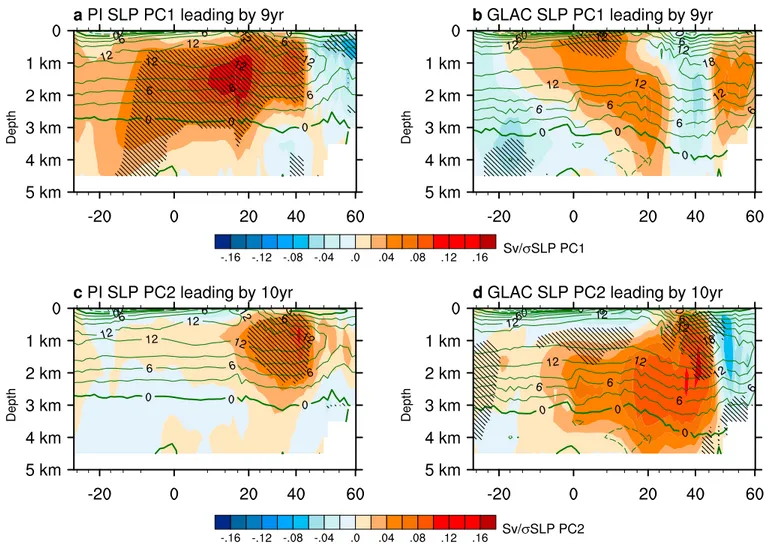
To investigate the relation between the AMOC and atmospheric variability, the meridional overturning stream function is regressed on the normalized SLP PCs with different time lags. Figures 3a and 3b show the 9‐year lag regression of the overturning stream function on the NAO index (SLP‐PC1) in PI and GLAC (refer to Figure S6 for time lags ranging from 0 to 10 years). The lagged overturning response in PI is significant between 10°S and 40°N, with the maximum regression coefficient of 0.13 Sv/σNAO(σNAOis the standard deviation of SLP‐PC1) at around 20°W and at 1‐to 2‐km depth (Figure 3a). This result indicates that the AMOC variability is tightly linked to the NAO under preindustrial conditions. Such a tight relationship is not observed in GLAC (Figure 3b). With the exception of the upper northern tropical Atlantic (from the equator to 10°N), there is no significant response of the overturning to the NAO in GLAC.

We now turn to the inﬂuence of the EAP on the AMOC. Previous studies suggested that the EAP should be included as an additional driver for the multidecadal AMOC variability (e.g., Msadek & Frankignoul, 2009;

Ruprich‐Robert & Cassou, 2015). This is supported by PI in which the EAP index (SLP‐PC2) drives significant variations in the overturning when leading by 10 years (Figure 3c; refer to Figure S7 for lags from 0 to 10 years). The influence of the EAP, however, is spatially restricted to the North Atlantic between 20°N and 45°N and the upper 2 km. The impact of the EAP on the AMOC is strongly intensified in GLAC and extends from 45°N to the equator (Figure 3d). The maximum regression coefficient amounts to 0.11 Sv/

Figure 3.Lag‐regressions (9‐year lag) of the overturning stream function on the normalized PC1 (NAO) for (a) PI and (b) GLAC. (c,d) As in (a) and (b) but PC2 (EAP) and 10‐year lag. The green contours indicate the annual mean overturning streamfunction. Hatching indicates signiﬁcance at the 95% conﬁdence interval usingpvalue test. NAO = North Atlantic Oscillation; EAP = East Atlantic pattern.

(6)

σEAPat 40°N and 2 km. In region 45–20°N, the response extends through the entire water column. Thus, the EAP is the mode of SLP variability that primarily drives the multidecadal AMOC variability in GLAC.

As reported by Biastoch et al. (2008), interannual to decadal variability of the AMOC in the midlatitude North Atlantic can be regarded as linear superposition of decadal and longer‐term thermohaline forcing variability and high‐frequency wind variability. Therefore, the JFMQ_netis regressed on SLP‐PC1 (NAO) in PI and on SLP‐PC2 (EAP) in GLAC (Figures 4a and 4b). When Q_net leads the AMOC by 10 years (Figures 4c and 4d), significant negative regression coefficients (color shading), that is, enhanced oceanic heat loss is observed over the convection sites (contours) in both PI and GLAC. In these regions, ocean density is enhanced and deep water formation intensified as suggested by the mixed layer depth (Figures 4e and 4f). TheQ_netpattern associated with the NAO (EAP) in Figure 4a (Figure 4b) and theQ_netpattern leading the AMOC by a decade shown in Figure 4c (Figure 4d) share similarities over the deep convection sites. This sug- gests that theQ_netanomalies associated with the NAO (EAP) drive the AMOC variations in PI (GLAC). In Figure 4.(a) Regressions of January‐February‐March (JFM) net surface heatflux (Q_net) on the normalized PC1 of JFM SLP (NAO) for PI and (b) on the normalized PC2 of JFM SLP (EAP) for GLAC. Lead (10‐yr lead)‐regressions (W/m²/Sv) of JFM Q_neton the AMOC index at 30°N for (c) PI and (d) GLAC. Lead (10‐yr lead)‐ regressions (m/Sv) of JFM mixed layer depth (MLD) on the AMOC index at 30°N for (e) PI and (f) GLAC. The green contours indicate JFM MLD. Stippling indicates significance at the 95% confidence interval using p‐value test. SLP = sea level pressure; NAO = North Atlantic Oscillation; EAP = East Atlantic pattern; AMOC = Atlantic meridional overturning circulation.

10.1029/2019GL082960

Geophysical Research Letters

(7)

contrast, theQ_netchanges in response to AMOC variations occur in the midlatitudes south of the convection sites (for PI see Figure 15 in Park et al., 2016).

To investigate the inﬂuence of ice sheet geometry and associated changes in land‐sea distribution on the internal atmospheric variability in more detail, four sensitivity experiments are carried out with the ECHAM5 atmosphere model in stand‐alone mode (Table S1). The results are presented for JFM in terms of the leading EOFs. When the atmosphere model is forced by GLAC (PI) ice sheets and either preindustrial or GLAC SST and sea ice conditions, the NAO (EOF1) and EAP (EOF2) patterns resemble those in GLAC (PI; Figures S8a–S8d). For example, an eastward shifted NAO pattern is simulated in the experiments forced by GLAC ice sheets, irrespective of whether preindustrial or GLAC SST and sea ice conditions are used or not (Figures S8b and S8d). The stand‐alone experiments with the atmosphere model suggest that the ice sheet conﬁguration is the most important factor determining the modes of atmospheric variability.

4. Summary and Discussion

This study investigates the multidecadal AMOC variability during the LGM and its driving factors by means of a version of the KCM. Our analysis conﬁrms previous results (e.g., Barrier et al., 2014; Biastoch et al., 2008;

Delworth et al., 2016; Kim et al., 2018) that under modern climate conditions multidecadal AMOC variations are mainly driven by surface heatﬂux (Qnet) anomalies associated with the NAO, withQ_netanomalies related to the EAP as an additional but much weaker driver. The impact of the NAO on the AMOC is virtually absent in GLAC, and the EAP‐relatedQ_netanomalies become the dominant driving force for the multidecadal AMOC variability. This change in forcing can be largely attributed to the presence of extensive continental ice sheets and related changes in land‐sea distribution, as conﬁrmed by dedicated experiments with the atmospheric component run in stand‐alone mode (Figure S8).

The multidecadal AMOC variability strengthens when the model is run under LGM conditions (GLAC) as compared to a reference run performed under preindustrial conditions (PI). Further research is needed to understand the increase in multidecadal AMOC variability. One reason could be the extensive deep convection site in GLAC, which is located south of Iceland. This is the region where the EAP imposes great inﬂu- ence on the AMOC through Ekman transport and especially Q_net (Barrier et al., 2014; Msadek &

Frankignoul, 2009). In PI, on the other hand, the deep convection site in the Labrador Sea is displaced to the east to the region South of Greenland. This model bias may reduce the sensitivity of the AMOC to NAO‐relatedQ_netvariability (Park et al., 2016).

Another question is the role of the oceanic mean state. Ocean‐only simulations suggest that buoyancyﬂuxes play a dominant role in driving the Labrador Sea Water formation and the subsequent AMOC changes (Barrier et al., 2014). Deep water formation and advection, however, strongly depend on the vertical and horizontal density gradients, thus affecting the thermohaline circulation (Steffen & D'Asaro, 2002). The implica- tion from these studies is that the much‐enhanced multidecadal AMOC variability simulated by the KCM in GLAC may be, at least partly, due to the different oceanic mean states.

In summary, simulations with the Kiel Climate Model suggest that the forcing for multidecadal AMOC variability changes under LGM conditions relative to modern times, with the EAP becoming the most important driver of the multidecadal AMOC variability during the LGM.

References

Balan, B., Gregory, J. M., Tailleux, R., Bigg, G. R., Blaker, A. T., Cameron, D. R., et al. (2011). High frequency variability of the Atlantic meridional overturning circulation.Ocean Science,7(4), 471–486. https://doi.org/10.5194/os‐7‐471‐2011

Barnston, A. G., & Livezey, R. E. (1987). Classiﬁcation, seasonality and persistence of low‐frequency atmospheric circulation patterns.

Monthly Weather Review,115(6), 1083–1126. https://doi.org/10.1175/1520‐0493(1987)115<1083:CSAPOL>2.0.CO;2

Barrier, N., Cassou, C., Deshayes, J., & Treguier, A.‐M. (2014). Response of North Atlantic Ocean circulation to atmospheric weather regimes.Journal of Physical Oceanography,44(1), 179–201. https://doi.org/10.1175/JPO‐D‐12‐0217.1

Bereiter, B., Eggleston, S., Schmitt, J., Nehrbass‐Ahles, C., Stocker, T. F., Fischer, H., et al. (2015). Revision of the EPICA dome C CO2record from 800 to 600 kyr before present.Geophysical Research Letters,42, 542–549. https://doi.org/10.1002/2014GL061957

Biastoch, A., Böning, C. W., Getzlaff, J., Molines, J.‐M., & Madec, G. (2008). Causes of interannual–decadal variability in the meridional overturning circulation of the midlatitude North Atlantic Ocean.Journal of Climate,21(24), 6599–6615. https://doi.org/10.1175/

2008JCLI2404.1

Böhm, E., Lippold, J., Gutjahr, M., Frank, M., Blaser, P., Antz, B., et al. (2015). Strong and deep Atlantic meridional overturning circulation during the last glacial cycle.Nature,517(7532), 73–76. https://doi.org/10.1038/nature14059

Acknowledgments

The suggestions of the two anonymous referees greatly improved an earlier version of the manuscript. This study was supported by the Integrated School of Ocean Sciences (ISOS) at the Excellence Cluster“The Future Ocean” at Kiel University sponsored by the German Science Foundation (DFG). We thank Stefan Hagemann and Christian Stepanek for their assistance with setting up the simulations. The integrations with the Kiel Climate Model (KCM) were conducted at the Computing Center of Kiel University (CAU). The KCM results presented in this study are available at Pangaea (https://doi.pangaea.de/10.1594/

PANGAEA.899572). The PMIP3 data output is available at this site (https://

esgf‐data.dkrz.de/search/cmip5‐dkrz/).

This is a contribution to the PalMod project funded by the German Ministry of Education and Research.

(8)

Braconnot, P., Harrison, S. P., Kageyama, M., Bartlein, P. J., Masson‐Delmotte, V., Abe‐Ouchi, A., et al. (2012). Evaluation of climate models using palaeoclimatic data.Nature Climate Change,2(6), 417–424. https://doi.org/10.1038/nclimate1456

Cayan, D. R. (1992). Latent and sensible heatﬂux anomalies over the northern oceans: The connection to monthly atmospheric circulation.

Journal of Climate,5(4), 354–369. https://doi.org/10.1175/1520‐0442(1992)005<0354:LASHFA>2.0.CO;2

Danabasoglu, G., Yeager, S. G., Kim, W. M., Behrens, E., Bentsen, M., Bi, D., et al. (2016). North Atlantic simulations in coordinated ocean‐

ice reference experiments phase II (CORE‐II). Part II: Inter‐annual to decadal variability.Ocean Modelling,97, 65–90. https://doi.org/

10.1016/J.OCEMOD.2015.11.007

Danabasoglu, G., Yeager, S. G., Kwon, Y.‐O., Tribbia, J. J., Phillips, A. S., & Hurrell, J. W. (2012). Variability of the Atlantic meridional overturning circulation in CCSM4.Journal of Climate,25(15), 5153–5172. https://doi.org/10.1175/JCLI‐D‐11‐00463.1

Delworth, T. L., Zeng, F., Delworth, T. L., & Zeng, F. (2016). The impact of the North Atlantic Oscillation on climate through its inﬂuence on the Atlantic Meridional Overturning Circulation.Journal of Climate,29(3), 941–962. https://doi.org/10.1175/JCLI‐D‐15‐

0396.1

Folland, C. K., Colman, A. W., Rowell, D. P., & Davey, M. K. (2001). Predictability of Northeast Brazil rainfall and real‐time forecast skill, 1987–98.Journal of Climate,14(9), 1937–1958. https://doi.org/10.1175/1520‐0442(2001)014<1937:PONBRA>2.0.CO;2

Folland, C. K., Palmer, T. N., & Parker, D. E. (1986). Sahel rainfall and worldwide sea temperatures, 1901–85.Nature,320(6063), 602–607.

https://doi.org/10.1038/320602a0

Hurrell, J. W. (1995). Decadal trends in the North Atlantic Oscillation: Regional temperatures and precipitation.Science,269(5224), 676–679 . https://doi.org/10.1126/science.269.5224.676

Jolliffe, I. (2002).Principal component analysis(2nd ed.). New York: Springer. Retrieved from http://cda.psych.uiuc.edu/statistical_learn- ing_course/

Justino, F., & Peltier, W. R. (2005). The glacial North Atlantic Oscillation.Geophysical Research Letters,32, L21803. https://doi.org/10.1029/

2005GL023822

Kageyama, M., Albani, S., Braconnot, P., Harrison, S. P., Hopcroft, P. O., Ivanovic, R. F., et al. (2017). The PMIP4 contribution to CMIP6—

Part 4: Scientiﬁc objectives and experimental design of the PMIP4‐CMIP6 Last Glacial Maximum experiments and PMIP4 sensitivity experiments.Geoscientiﬁc Model Development,10(11), 4035–4055. https://doi.org/10.5194/gmd‐10‐4035‐2017

Kanzow, T., Cunningham, S. A., Johns, W. E., Hirschi, J. J.‐M., Marotzke, J., Baringer, M. O., et al. (2010). Seasonal variability of the Atlantic meridional overturning circulation at 26.5°N.Journal of Climate,23(21), 5678–5698. https://doi.org/10.1175/2010JCLI3389.1 Kim, W. M., Yeager, S., Chang, P., & Danabasoglu, G. (2018). Low‐frequency North Atlantic climate variability in the Community Earth

System Model large ensemble.Journal of Climate,31(2), 787–813. https://doi.org/10.1175/JCLI‐D‐17‐0193.1

Klockmann, M., Mikolajewicz, U., & Marotzke, J. (2016). The effect of greenhouse gas concentrations and ice sheets on the glacial AMOC in a coupled climate model.Climate of the Past,12(9), 1829–1846. https://doi.org/10.5194/cp‐12‐1829‐2016

Lippold, J., Luo, Y., Francois, R., Allen, S. E., Gherardi, J., Pichat, S., et al. (2012). Strength and geometry of the glacial Atlantic Meridional Overturning Circulation.Nature Geoscience,5(11), 813–816. https://doi.org/10.1038/ngeo1608

Madec, G. (2008).NEMO ocean engine.Note du Pole de modélisation 27, Institut Pierre‐Simon Laplace(193 pp.). Retrieved from http://www.

nemo‐ocean.eu/content/download/5302/31828/ﬁle/NEMO_book.pdf

Marzocchi, A., & Jansen, M. F. (2017). Connecting Antarctic sea ice to deep‐ocean circulation in modern and glacial climate simulations.

Geophysical Research Letters,44, 6286–6295. https://doi.org/10.1002/2017GL073936

McManus, J. F., Francois, R., Gherardi, J.‐M., Keigwin, L. D., & Brown‐Leger, S. (2004). Collapse and rapid resumption of Atlantic meridional circulation linked to deglacial climate changes.Nature,428(6985), 834–837. https://doi.org/10.1038/nature02494

Medhaug, I., Langehaug, H. R., Eldevik, T., Furevik, T., & Bentsen, M. (2012). Mechanisms for decadal scale variability in a simulated Atlantic meridional overturning circulation.Climate Dynamics,39(1–2), 77–93. https://doi.org/10.1007/s00382‐011‐1124‐z Menary, M. B., Park, W., Lohmann, K., Vellinga, M., Palmer, M. D., Latif, M., & Jungclaus, J. H. (2012). A multimodel comparison of

centennial Atlantic meridional overturning circulation variability.Climate Dynamics,38(11–12), 2377–2388. https://doi.org/10.1007/

s00382‐011‐1172‐4

Mix, A. C., Bard, E., & Schneider, R. (2001). Environmental processes of the ice age: Land, oceans, glaciers (EPILOG).Quaternary Science Reviews,20(4), 627–657. https://doi.org/10.1016/S0277‐3791(00)00145‐1

Msadek, R., & Frankignoul, C. (2009). Atlantic multidecadal oceanic variability and its inﬂuence on the atmosphere in a climate model.

Climate Dynamics,33(1), 45–62. https://doi.org/10.1007/s00382‐008‐0452‐0

Muglia, J., & Schmittner, A. (2015). Glacial Atlantic overturning increased by wind stress in climate models.Geophysical Research Letters, 42, 9862–9868. https://doi.org/10.1002/2015GL064583

Park, T., Park, W., & Latif, M. (2016). Correcting North Atlantic sea surface salinity biases in the Kiel Climate Model: Inﬂuences on ocean circulation and Atlantic multidecadal variability.Climate Dynamics,47(7–8), 2543–2560. https://doi.org/10.1007/s00382‐016‐

2982‐1

Park, W., Keenlyside, N., Latif, M., Ströh, A., Redler, R., Roeckner, E., & Madec, G. (2009). Tropical Paciﬁc climate and its response to global warming in the Kiel Climate Model.Journal of Climate,22(1), 71–92. https://doi.org/10.1175/2008JCLI2261.1

Pausata, F. S. R., Li, C., Wettstein, J. J., Kageyama, M., & Nisancioglu, K. H. (2011). The key role of topography in altering North Atlantic atmospheric circulation during the last glacial period.Climate of the Past,7(4), 1089–1101. https://doi.org/10.5194/cp‐7‐1089‐2011 Pausata, F. S. R., Li, C., Wettstein, J. J., Nisancioglu, K. H., & Battisti, D. S. (2009). Changes in atmospheric variability in a glaicial climate

and the impacts on proxy data: A model intercomparison.Climate of the Past,5(3), 489–502. https://doi.org/10.5194/cp‐5‐489‐2009 Roeckner, E., Bäuml, G., Bonaventura, L., Brokopf, R., Esch, M., Giorgetta, M., et al. (2003). The atmospheric general circulation model

ECHAM 5. PART I: Model description.Max‐Planck‐Institut für Meteorologie,349. Retrieved from http://pubman.mpdl.mpg.de/pubman/

item/escidoc:995269/component/escidoc:995268/Report‐349.pdf

Ruprich‐Robert, Y., & Cassou, C. (2015). Combined inﬂuences of seasonal East Atlantic Pattern and North Atlantic Oscillation to excite Atlantic multidecadal variability in a climate model.Climate Dynamics,44(1–2), 229–253. https://doi.org/10.1007/s00382‐014‐2176‐7 Steffen, E., & D'Asaro, L. (2002). Deep convection in the Labrador Sea as observed by Lagrangianﬂoats.Journal of Physical Oceanography,

32(2), 475–492. https://doi.org/10.1175/1520‐0485(2002)032<0475:DCITLS>2.0.CO;2

Sutton, R. T., & Hodson, D. L. R. (2005). Atlantic Ocean forcing of North American and European summer climate.Science,309(5731), 115–118. https://doi.org/10.1126/SCIENCE.1109496

Valcke, S. (Ed.) (2006).OASIS3 User Guide (PRISM_2–5).CERFACS Technical Report TR/CMGC/06/73, PRISM Report No 3(60 pp.).

Toulouse, France. Retrieved from http://www.prism.enes.org/Publications/Reports/oasis3_UserGuide_T3.pdf

Wang, C., & Lee, S.‐K. (2009). Co‐variability of tropical cyclones in the North Atlantic and the eastern North Paciﬁc.Geophysical Research Letters,36, L24702. https://doi.org/10.1029/2009GL041469

10.1029/2019GL082960

Geophysical Research Letters

(9)

Weber, S. L., Drijfhout, S. S., Abe‐Ouchi, A., Cruciﬁx, M., Eby, M., Ganopolski, A., et al. (2007). The modern and glacial overturning circulation in the Atlantic Ocean in PMIP coupled model simulations.Climate of the Past,3(1), 51–64. https://doi.org/10.5194/cp‐3‐51‐2007 Wei, W., & Lohmann, G. (2012). Simulated Atlantic Multidecadal Oscillation during the Holocene.Journal of Climate,25(20), 6989–7002.

https://doi.org/10.1175/JCLI‐D‐11‐00667.1

Zanchettin, D., Rubino, A., Matei, D., Bothe, O., & Jungclaus, J. H. (2013). Multidecadal‐to‐centennial SST variability in the MPI‐ESM simulation ensemble for the last millennium.Climate Dynamics,40(5–6), 1301–1318. https://doi.org/10.1007/s00382‐012‐1361‐9