1
Sub-decadal North Atlantic Oscillation Variability in Observations and the Kiel Climate 1
Model 2
A. Reintges1, M. Latif1,2, and W. Park1 3
1GEOMAR Helmholtz Centre for Ocean Research Kiel, Kiel, Germany 4
2University of Kiel, Kiel, Germany 5
GEOMAR Helmholtz Centre for Ocean Research Kiel 6
Düsternbrooker Weg 20, 24105 Kiel, Kiel, Germany 7
e-mail: areintges@geomar.de 8
telephone: +49 431 600-4007 9
fax: +49 431 600-4052 10
11 12 13 14 15 16 17 18 19 20 21
NOTE: This is a post-peer-review, pre-copyedit version of an article published in Climate 22
Dynamics. The final authenticated version is available online at:
23
https://link.springer.com/article/10.1007/s00382-016-3279-0 24
Please cite as Reintges, A., Latif, M. and Park, W. (2017) Sub-decadal North Atlantic 25
Oscillation variability in observations and the Kiel Climate Model. Climate Dynamics 26
48:3475–3487. doi:10.1007/s00382-016-3279-0 27
2
Sub-decadal North Atlantic Oscillation Variability in Observations and the Kiel Climate 28
Model 29
Annika Reintges, Mojib Latif, and Wonsun Park 30
Abstract 31
The North Atlantic Oscillation (NAO) is the dominant mode of winter climate variability in 32
the North Atlantic sector. The corresponding index varies on a wide range of timescales, from 33
days and months to decades and beyond. Sub-decadal NAO variability has been well 34
documented, but the underlying mechanism is still under discussion. Other indices of North 35
Atlantic sector climate variability such as indices of sea surfaceand surface air temperature or 36
Arctic sea ice extent also exhibit pronounced sub-decadal variability. Here, we use sea surface 37
temperature and sea level pressure observations, and the Kiel Climate Model (KCM) to 38
investigate the dynamics of the sub-decadal NAO variability. The sub-decadal NAO 39
variability is suggested to originate from dynamical large-scale air-sea interactions. The 40
adjustment of the Atlantic Meridional Overturning Circulation to previous surface heat flux 41
variability provides the memory of the coupled mode. The results stress the role of coupled 42
feedbacks in generating sub-decadal North Atlantic sector climate variability, which is 43
important to multiyear climate predictability in that region.
44 45
Keywords: North Atlantic climate variability; North Atlantic Oscillation (NAO); Sub-decadal 46
variability; Atmosphere-ocean interaction; Atlantic Meridional Overturning Circulation 47
(AMOC) 48
3 1. Introduction
49
The North Atlantic Oscillation (NAO) is a large-scale seesaw in atmospheric mass between 50
the Azores high and the Icelandic low (Hurrell 1995; Visbeck et al. 2001; Hurrell et al. 2003).
51
Variations in the NAO are associated with strong changes in wintertime storminess over the 52
North Atlantic, and European and North American surface air temperature (SAT) and 53
precipitation, and thus have major economic impacts. A statistically significant sub-decadal 54
peak can be identified in the power spectrum of the traditional NAO index (Czaja and 55
Marshall 2001; Fye et al. 2006). Statistically significant sub-decadal peaks are also seen in the 56
power spectra of other quantities observed in the North Atlantic sector (Deser and Blackmon 57
1993; Sutton and Allen 1997; Czaja and Marshall 2001; Fye et al. 2006; Álvarez-García et al.
58
2008).
59
The sub-decadal variability in the North Atlantic sector is distinct from the longer-term 60
multidecadal variability in that region (Álvarez-García et al. 2008), which is associated with 61
the Atlantic Multidecadal Oscillation/Variability (AMO/V) (Knight et al. 2005). In this study, 62
we only address the sub-decadal variability. Different competing hypotheses have been put 63
forward to explain the North Atlantic sector sub-decadal variability. It has been linked, for 64
instance, to Arctic sea ice (Deser and Blackmon 1993), to advection by the mean ocean 65
circulation (Sutton and Allen 1997), to the wind-driven ocean circulation (Czaja and Marshall 66
2001; Marshall et al. 2001), to the Atlantic Meridional Overturning Circulation (AMOC) 67
(Eden and Greatbatch 2003; Álvarez-García et al. 2008), and to stochastic resonance 68
(Saravanan and McWilliams 1997, 1998). Further, it is controversial whether the North 69
Atlantic sub-decadal climate variability observed in different variables is part of one single 70
dynamical mode of the coupled ocean-atmosphere-sea ice system or is composed of different 71
modes each originating from different physical processes.
72
4
Here, we investigate the origin of the sub-decadal NAO variability and related climate 73
variability in the North Atlantic sector by analyzing historical observations and a millennial 74
control integration of the Kiel Climate Model (KCM), a coupled ocean-atmosphere-sea ice 75
general circulation model. By definition, time-varying external forcing is not considered in 76
such control integration and variability is only internally generated. Section 2 provides 77
information about the observational data, the climate model and the experimental setup, and 78
the statistical method for the identification of the sub-decadal mode in the different datasets.
79
In Section 3, by jointly discussing the observations and the results from the KCM, we present 80
the mechanism that is suggested to produce the sub-decadal NAO variability. Summary of the 81
major findings and main conclusions are presented in Section 4.
82
2. Data and methodology 83
Observational data 84
We use the observed station-based winter (December through March, DJFM) NAO index 85
during 1864-2014 from https://climatedataguide.ucar.edu/climate-data/hurrell-north-atlantic- 86
oscillation-nao-index-station-based. The station-based NAO index is defined as the difference 87
of the normalized sea level pressure (SLP) anomaly time series between Lisbon (Portugal;
88
38.72°N, 9.17°W) and Stykkisholmur/Reykjavik (Iceland; 65.07°N, 22.72°W). The climate 89
model’s NAO index is computed in an analogous manner from the nearest grid points. The 90
station-based index also well describes the model’s NAO variability (see supplementary Fig.
91
S1).
92
In the regression and cross-correlation analyses presented below, gridded sea surface 93
temperatures (SSTs, ERSST V3b) provided for January 1854 – April 2015 are from 94
http://www.ncdc.noaa.gov/ersst/. A dipolar SST index is defined from the observed SSTs by 95
subtracting mid-latitudinal from subpolar North Atlantic SST anomalies (see boxes in Fig. 1b;
96
5
according to this convention, a negative index means an enhanced meridional SST gradient).
97
The KCM’s dipolar SST index is computed in an analogous manner.
98
Gridded sea level pressures data (SLPs, HadSLP2) provided for the time period January 1850 99
– December 2014 are obtained from http://www.metoffice.gov.uk/hadobs/hadslp2/. The 100
common period 1864 – 2014 is used when computing correlations and regressions of the 101
SSTs and SLPs with respect to the NAO index. Measurements of the AMOC index at 26.5°N 102
from the RAPID array are downloaded from http://www.rapid.ac.uk/rapidmoc/ (Smeed et al.
103
2015). The RAPID data have been widely used during the recent years; for example, by 104
Bryden et al. (2014) and Cunningham et al. (2013), two studies which are relevant here. The 105
AMOC index is provided for the period April 2004 – March 2015. We use the annual mean 106
values of the AMOC index for the eleven years during 2004 – 2014.
107
Coupled model and experiments 108
The Kiel Climate Model (KCM; see Park et al. 2009) is an atmosphere-ocean-sea ice general 109
circulation model. It consists of the ECHAM5 atmosphere general circulation model on a T31 110
horizontal grid (3.75° x 3.75°) with 19 vertical levels, which is coupled through the OASIS 111
coupler to the NEMO ocean-sea ice model on a 2˚ Mercator mesh amounting on average to 112
1.3° resolution. Enhanced meridional resolution of 0.5° is employed in the equatorial region 113
and the ocean model is run with 31 levels. The KCM has been used in many climate 114
variability and response studies. A list of studies conducted with the KCM can be obtained 115
from http://www.geomar.de/en/research/fb1/fb1-me/research-topics/climate-modelling/kcms/.
116
We analyze the last 700 years of output from a millennial present-day control simulation after 117
skipping the first 300 years, which has been initialized with Levitus climatology. The 118
climatology of selected quantities is shown in Fig. 1. Like many other climate models, the 119
KCM suffers from large biases in the North Atlantic region (see supplementary Fig. S2 and 120
S3). In particular, a cold SST bias is observed in the mid-latitudes, which largely originates 121
6
from an incorrect path of the North Atlantic Current (Drews et al. 2015). We additionally 122
investigate 700 years from an integration of the ECHAM5 atmosphere general circulation 123
model coupled to a slab ocean model with a constant depth of 50 m. In this reduced coupled 124
model, changes in ocean circulation are completely ignored. Comparison of the fully coupled 125
(KCM) integration with the slab ocean coupled integration provides information about the 126
importance of ocean dynamical feedbacks for the sub-decadal NAO variability in the KCM.
127
Finally, the ECHAM5 model version employed by the KCM is integrated in an uncoupled 128
mode with prescribed SSTs. Two experiments are performed, each 99 years long. The first 129
experiment is a control run in which only the observed monthly SST climatology drives the 130
model. In the second experiment, the observed winter (DJFM) SST anomalies associated with 131
the positive phase of the sub-decadal NAO mode (see Fig. 7a, right panel) are superimposed 132
on the observed SST climatology globally. The differences between the two experiments 133
provide information about whether and how the SST anomalies feed back onto the 134
atmosphere and thus yield some information about the role of air-sea coupling in generating 135
the sub-decadal NAO mode. The atmospheric response is defined as the difference between 136
the two long-term means (experiment minus control), where the long-term mean is computed 137
from all 99 DJFM values. A t-test provides the statistical significance of the response.
138
Statistical methods 139
Singular Spectrum Analysis (SSA; see Vautard and Ghil 1989) is applied here to derive 140
oscillatory modes from the observations and the model data. The results of the SSA may be 141
sensitive to the choice of parameters. In order to investigate such sensitivity different 142
variables and window lengths have been applied, and the results are rather robust. In the SSAs 143
of the observed NAO index and the observed (dipolar) SST index, both covering about 150 144
years, the window length is 15 years and only these results are shown below. Sensitivity tests 145
using a window length of 20 years were performed. The results are virtually unchanged, 146
7
suggesting robustness in the results from the observational analyses. Furthermore, sub- 147
decadal modes are identified from SSA applied separately to the observed NAO index and the 148
observed (dipolar) SST index. With regard to the KCM, SLP, geopotential, storm track, SST, 149
surface heat flux and AMOC indices from the model have been individually used in the SSA, 150
and they all yield the same sub-decadal period of 9 years. KCM-results shown below are from 151
SSAs employing a window length of 100 years. Sensitivity tests conducted using several 152
window lengths in the range of 70 to 150 years yield similar results. Thus, we can confidently 153
state that at least in the model, a statistically significant sub-decadal mode is simulated in the 154
North Atlantic sector that has expressions in both the atmosphere and the ocean.
155
Cross-correlation and linear regression analyses were performed to investigate the links 156
between different variables. In the calculation of the confidence limits for the correlation 157
coefficients, we use a t-test based on the effective number of degrees of freedom which is 158
estimated from the decorrelation time of each time series (Leith 1973) separately, explaining 159
the differing confidence limits in the plots shown below. The decorrelation time is defined 160
here as the e-folding timescale of the time series’ auto-correlation function. By multiplying 161
the critical correlation coefficient with the standard deviation of the variable under 162
consideration we obtain the threshold for the corresponding regression coefficient.
163
3. Results 164
Statistical analyses 165
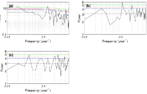
We first compute the power spectrum of the observed winter-NAO index during 1864-2014.
166
Sub-decadal NAO variability is statistically significant at the 99%-confidence level in the 167
observations (Fig. 2a), which is one of the main motivations for this study. We next computed 168
the winter-NAO index spectra from the two coupled model simulations. Differences in the 169
spectra computed from the two simulations depict the role of ocean dynamics in influencing 170
8
the NAO. Statistically significant sub-decadal NAO variability is observed in the power 171
spectrum of the coupled simulation employing a dynamical ocean model (Fig. 2b), the KCM, 172
but not in that of the coupled integration with the slab ocean model (Fig. 2c). The existence 173
(absence) of the sub-decadal NAO mode in the power spectrum computed from the coupled 174
simulation with the dynamical (slab) ocean model was verified by repeating the spectral 175
analysis with different window types and window lengths. On the contrary, the peaks seen at 176
25 years and 4 years in Fig. 2c are not robust. The lack of enhanced sub-decadal NAO 177
variability in the coupled simulation with the slab ocean model suggests that dynamical ocean 178
processes, through their influence on SST, is essential to produce the sub-decadal NAO mode 179
in the KCM. We return to this point below.
180
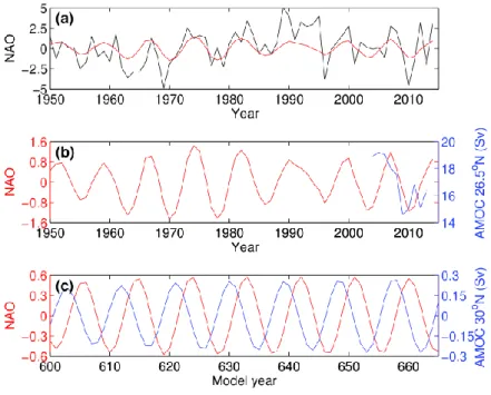
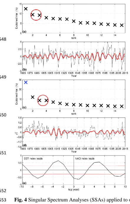
Consistent with the power spectrum presented above (Fig. 2a), the SSA of the observed 181
winter-NAO index of 1864-2014 reveals a sub-decadal oscillatory mode with a period of 8 182
years (red line in Fig. 3a,b) that accounts for 18% of the total variance (Fig. 4a). This SSA 183
mode is, however, not statistically significant against red noise at the 95% - confidence limit.
184
We present the reconstructed NAO index together with the AMOC index at 26.5°N from the 185
RAPID array in Fig. 3b. The evolution of the observed AMOC index depicts similar sub- 186
decadal variability (Bryden et al. 2014; Cunningham et al. 2013) as the reconstructed NAO 187
index. However, the AMOC record is very short only covering about a decade, which does 188
not allow drawing any inferences about causality and the reason for additionally investigating 189
the sub-decadal NAO variability simulated by the KCM. As will be discussed in detail below, 190
the KCM depicts a close connection between the AMOC and the NAO at sub-decadal 191
timescales (Fig. 3c) such that the former leads the latter by about a year. This suggests the 192
assumption that the observed sub-decadal AMOC signal is part of an oscillation in the North 193
Atlantic region and related to the NAO.
194
9
We next perform SSA on the KCM’s NAO index, which yields a leading oscillatory sub- 195
decadal mode with a period of 9 years (red line in Fig. 3c) accounting for about 4% of the 196
total variance (Fig. 5a). We note that the explained variance strongly depends on the window 197
length, while the existence of the sub-decadal SSA mode does not. When choosing a window 198
length of 15 years, as in the observational analyses, the explained variance is similar to that 199
obtained from the SSA of the observed NAO index. For example, using only the last 150 200
years from the model and a window length of 15 years yields a sub-decadal NAO mode that 201
accounts for about 20 % of the variance. Further, since SSA provides modes which are 202
sharply peaked in frequency space, the variance accounted for by SSA modes is generally 203
considerably lower in comparison to other statistical techniques such as Empirical Orthogonal 204
Function (EOF) analysis which covers a larger frequency range. The sub-decadal NAO mode 205
obtained from the KCM (Fig. 3c) is statistically significant against red noise at the 95 % 206
confidence limit. We observedin the KCM a strong amplitude modulation of the sub-decadal 207
NAO variability on centennial timescales (red curve in Fig. 5b). No sub-decadal mode is 208
obtained from the SSA of the NAO index simulated in the coupled integration with the slab 209
ocean model (not shown), which reinforces the findings from the investigation of the power 210
spectra (Fig. 2). In the coupled experiment in which the dynamical ocean model is replaced by 211
a slab ocean model, the NAO index does not exhibit statistically significant sub-decadal 212
variability above the background spectrum (Fig. 2c). Furthermore, applying SSA to the NAO 213
index does not reveal a statistically significant sub-decadal NAO mode. However, a peak at 214
multidecadal timescales is seen in the spectrum of the NAO index obtained from the coupled 215
integration with the slab ocean. This peak appears not to be robust, because it is neither 216
supported by SSA nor seen in the power spectra of other variables (not shown). The 217
comparison of the KCM results with those of the coupled slab ocean model integration 218
demonstrates that ocean dynamical processes are necessary to produce the sub-decadal NAO 219
mode in the KCM.
220
10 Sub-decadal mode surface patterns
221
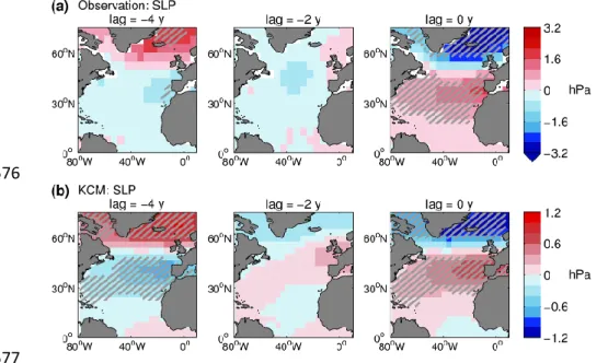
The sub-decadal NAO-index reconstructions are used as indices to compute regression 222
patterns of SLP anomalies during winter (DJFM) from the observations and the KCM. Both 223
evolutions, that obtained from observations (Fig. 6a) and that from the KCM (Fig. 6b), depict 224
a transition from the negative polarity of the NAO at lag -4yr to its positive polarity at lag 0yr.
225
At lag -2yr, SLP anomalies are considerably weaker, so that the sub-decadal SLP variability 226
approximately takes the form of a standing oscillation in the observations and in the KCM.
227
Notable differences between the SLP regression patterns are also seen, especially at lag -2yr.
228
However, this mostly concerns non-significant features. The gross features of the time-space 229
structure are similar, supporting that the model is reasonably well capturing the observed sub- 230
decadal SLP variability.
231
Lag-regressions of sea surface temperature (SST) anomalies during DJFM are computed next 232
(Fig. 7), again upon the two NAO-index reconstructions. In both the observations (Fig. 7a) 233
and the KCM (Fig. 7b), negative SST anomalies appear in the mid-latitudes at lag -4yr, which 234
intensify during the subsequent two years. In the Labrador and Irminger Seas, negative SST 235
anomalies emerge at lag -1yr in both datasets (not shown). At lag 0yr, i.e. when the sub- 236
decadal NAO mode is in its positive phase, the negative SST anomaly in the subpolar North 237
Atlantic has strengthened, while in the mid-latitudes, the negative SST anomaly is replaced by 238
a positive SST anomaly which emanated from the western boundary.
239
Mechanism in the KCM 240
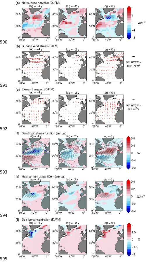
In order to gain further insight into the mechanism behind the sub-decadal NAO variability, 241
we now investigate the model results in more detail. Consistent with observations (Czaja 242
2001; Cayan 1992), the net surface heat flux anomalies (Fig. 8a) tend to drive the SST 243
anomalies in the subpolar and mid-latitude North Atlantic during the two extreme phases (lag 244
11
-4yr, lag 0yr) of the sub-decadal NAO mode. At these lags, the anomalous wind stress (Fig.
245
8b) through its curl forces anomalous Ekman transports (Fig. 8c), and these contribute to the 246
generation of the SST anomalies in the centers of action. At lag -3yr (not shown) and lag -2yr, 247
the net heat flux anomalies, though not being statistically significant, still tend to damp the 248
SST anomalies, especially in the mid-latitude North Atlantic. Furthermore, wind stress 249
anomalies are weak in this transition phase of the sub-decadal NAO mode (Fig. 8b). Thus, the 250
strong negative SST anomalies simulated by the KCM at lag -2yr must originate from ocean 251
dynamical processes. The barotropic streamfunction anomalies associated with the sub- 252
decadal NAO mode depict statistically significant regressions at all lags (Fig. 8d). An 253
“intergyre” gyre (Marshall et al. 2001) develops at lag -4yr and persists until lag -2yr, pushing 254
the subpolar-gyre boundary southward. This favors sea surface cooling in the mid-latitudes 255
with a time delay of one to two years, which constitutes a positive feedback on the SST 256
anomalies in that region.
257
A delayed negative feedback is provided by the AMOC which responds to the dipolar heat 258
flux anomalies prevailing during the negative extreme of the sub-decadal NAO mode at lag - 259
4yr (Fig. 8a). Statistically significant upper ocean (0-500m) heat content anomalies (Fig. 8e) 260
are simulated by the model in the mid-latitudes at lag -4yr. At lag -2yr, a small heat content 261
signal of opposite sign develops in the west and follows the path of the KCM’s North Atlantic 262
Current, eventually reversing the SST tendency in the mid-latitude North Atlantic. This heat 263
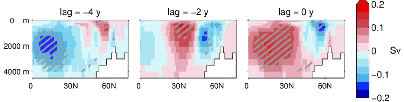
content signal is attributed to the concurrent changes in the AMOC. The overturning 264
streamfunction depicts a well-developed dipolar anomaly with a node near 45°N at lag-2yr 265
(Fig. 9). The positive AMOC anomaly centered near 30°N enhances the transport of warm 266
water in the upper ocean from the subtropics to the mid-latitudes. Further to the north, 267
negative SST and heat content anomalies develop at lag -1yr (not shown) and reach full 268
12
strength at lag 0yr (Fig. 7, 8). At this time, we find increased sea ice concentration in the 269
western subpolar North Atlantic (Fig. 8f).
270
To sharpen the role of the AMOC in the KCM’s sub-decadal NAO variability, SSA was 271
performed on an AMOC index defined as the maximum overturning streamfunction at 30°N 272
(black curve in Fig. 5g). The leading oscillatory SSA mode, comprising basin-wide changes 273
of the AMOC (not shown), is multidecadal (Park and Latif 2008) (rank 1 and 2 in Fig. 5f) and 274
not of relevance here. The next energetic SSA mode accounting for about 8% of the total 275
variance is significant against a red noise process and sub-decadal (Fig. 5f,g) with a period of 276
9 years. We reconstructed the AMOC index using this SSA mode (red curve in Fig. 5g) and 277
lag-correlated the reconstructed AMOC index with the sub-decadal NAO index reconstruction 278
(red curve in Fig. 5b). The two indices, which have been derived from independent statistical 279
analyses, are strongly lag-correlated (Fig. 5h), suggesting they are part of the same physical 280
mode. The largest correlation (r = 0.74) is attained when the (reconstructed) AMOC index 281
leads the (reconstructed) NAO index by one year (see also Fig. 3c). This suggests that the 282
AMOC is instrumental, through its impact on SST, in driving the sub-decadal NAO 283
variability in the KCM.
284
Air-sea coupling 285
Conceptually, the sub-decadal variability simulated by the KCM can be understood as a 286
delayed action oscillator (Marshall et al. 2001). We hypothesize that the dipolar overturning 287
anomaly, with a time delay, strengthens the meridional SST gradient between the subpolar 288
and mid-latitude North Atlantic. This in turn drives the phase change of the sub-decadal NAO 289
mode to its positive polarity. To test this hypothesis a dipolar SST index is calculated from 290
both the observations and the model by subtracting mid-latitudinal from subpolar SST 291
anomalies (the SSTs were averaged over the boxes shown in Fig. 1b and Fig. 7). According to 292
this definition, a stronger meridional SST gradient is associated with a negative index. SSA 293
13
applied to the dipolar SST indices calculated from the observations and the model yields sub- 294
decadal modes with the same periods as those obtained from the SSA of the NAO indices 295
(Fig. 4c,d; Fig. 5c,d), lending further support to the assumption that the sub-decadal 296
oscillation is a robust mode in both the observations and the model. We correlate next the sub- 297
decadal SSA-mode reconstructions of the dipolar SST indices with the sub-decadal SSA- 298
mode reconstructions of the NAO indices (Fig. 4b, 5b). The cross-correlation functions 299
calculated from the observations (Fig. 4e) and the model (Fig. 5e) are very similar. They both 300
clearly depict the sub-decadal periodicity and exhibit statistically significant negative cross- 301
correlation (above the 95 % level) at lag 0yr. This supports the conjecture that the sub-decadal 302
NAO variability involves large-scale ocean-atmosphere coupling, with a stronger meridional 303
SST gradient driving a stronger NAO index and vice versa.
304
As shown in Fig. 5, the dipolar SST index and NAO index SSA-mode reconstructions are 305
highly correlated. The fact that a sub-decadal periodicity can be identified in the NAO index 306
by itself supports the notion that the sub-decadal NAO variability is part of a coupled ocean- 307
atmosphere mode, assuming that the atmosphere by itself does not produce a sub-decadal 308
cycle. The atmospheric response to mid-latitudinal SST anomalies is a controversial topic and 309
not well understood. This is demonstrated, for example, by the diversity of model results. The 310
coarse horizontal resolution (T31) of the atmospheric component (ECHAM5) of the KCM 311
does not a priori inhibit the atmosphere model to responding to the dipolar SST anomalies.
312
The spatial scale of the dipolar SST anomaly, exhibiting opposite changes in the subpolar and 313
mid-latitudinal Atlantic, is sufficiently large to be resolved by the atmosphere model.
314
One needs to bear in mind in this context that consistent with observations, a positive phase of 315
the NAO is associated with surface heat flux anomalies (Fig. 8a) which tend to cool the 316
subpolar North Atlantic and warm the region to the south of it. These heat flux anomalies tend 317
to reinforce the dipolar SST anomaly in the KCM, constituting a positive feedback. Consistent 318
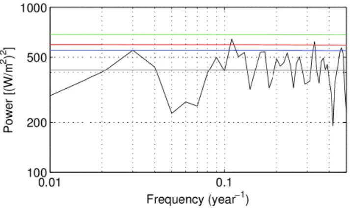
14
with the spectral analyses presented above, the power spectrum of the heat flux anomalies 319
averaged over the subpolar North Atlantic (48°–15°W/43°–58°N) depicts a peak at 9 years 320
that is statistically significant at the 99 % level (Fig. 10). Furthermore, SSA applied to that 321
heat flux index yields a statistically significant oscillatory mode with a period of 9 years (not 322
shown), which further supports the conjecture that air-sea coupling is important in producing 323
the sub-decadal NAO mode.
324
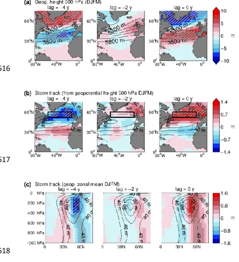
We next examine the vertical structure of the atmospheric changes associated with the sub- 325
decadal NAO mode. The 500 hPa geopotential height anomalies, as shown by lag-regression 326
patterns (Fig. 11a) calculated upon the sub-decadal NAO SSA-mode reconstruction (as in Fig.
327
8), have a similar horizontal structure as the SLP anomalies, indicating an equivalent 328
barotropic vertical structure and suggesting an eddy-mediated response. As in the SLP 329
anomaly field, the changes in the centers of action of the 500 hPa height anomaly field are 330
statistically significant. The height response goes along with statistically significant 331
regressions in the storm track at 500 hPa (Fig. 11b), as defined by the standard deviation of 332
the 12-hourly band-pass filtered (2.5 - 8 days) height anomalies. The mean storm track over 333
the North Atlantic is centered near 45°N (Fig. 1k and contours in Fig. 11b). During the 334
negative NAO phase (lag -4yr), the storm track shifts southward, during the positive NAO 335
phase (lag 0yr) poleward (Fig. 11b). The vertical structure of the regressions calculated from 336
the zonally (80°W-10°E) averaged storm track reveals statistically significant changes in 337
synoptic activity up to the 500 hPa level (Fig. 11c).
338
Forced atmosphere model experiments 339
In order to investigate the atmospheric response to the dipolar SST anomaly in more detail, 340
we now turn to the forced integrations with the ECHAM5 atmosphere model. When the 341
atmosphere model is forced by the SST anomalies associated with the positive phase of the 342
(observed) sub-decadal NAO mode (Fig. 7a, right panel; Fig. S4a), a statistically significant 343
15
atmospheric response is simulated that is consistent with the results described above. For 344
example, the SLP response pattern (Fig. S4b) is rather similar to the observed pattern (Fig. 6a, 345
right panel) and the KCM pattern (Fig. 6b, right panel) that are associated with the sub- 346
decadal NAO variability. Furthermore, the heat flux response pattern simulated in the forced 347
atmosphere model experiment (Fig. S4c) confirms the positive feedback postulated above on 348
the basis of the KCM results (Fig. 8a, right panel). Moreover, the pressure response in the 349
forced experiment is equivalent barotropic (not shown), as it is in the KCM (Fig. 11a, right 350
panel). Additional sensitivity experiments (not shown) reveal that it is the SST anomalies in 351
the North Atlantic north of 25°N that are most important in driving the NAO-like atmospheric 352
response. It is, however, beyond the scope of this paper to discuss the atmospheric response at 353
great length. What is important here is that the ECHAM5 atmosphere model is sensitive to the 354
dipolar SST anomaly associated with the sub-decadal NAO variability and reproduces the 355
coupled model patterns. In particular, the forced atmosphere model experiment supports the 356
existence of a positive atmosphere-ocean feedback. Atmospheric sensitivity to AMOC-related 357
dipolar SST changes in the North Atlantic also has been recently reported from another 358
climate model (Frankignoul et al. 2015). The limited observational data also support such an 359
atmospheric sensitivity to mid-latitudinal SST anomalies (Bryden et al. 2014; Czaja and 360
Frankignoul 1999; Czaja and Frankignoul 2002).
361
4. Summary and Discussion 362
We have investigated the sub-decadal variability of the North Atlantic Oscillation (NAO) and 363
of other quantities in the North Atlantic sector. Such sub-decadal variability in the North 364
Atlantic sector is well documented from observations. The Kiel Climate Model (KCM) 365
simulates such a North Atlantic sub-decadal variability in a millennial control run, suggesting 366
it could be internal in nature and does not require external forcing. It is suggested on the basis 367
of the coupled model results that the sub-decadal NAO mode is part of a coupled mode of the 368
16
North Atlantic ocean-atmosphere-sea ice system. More specifically, the sub-decadal climate 369
variability in the North Atlantic sector is the result of positive ocean-atmosphere feedback and 370
delayed negative ocean dynamical feedback. The latter is shown by an additional coupled 371
model integration in which the dynamical ocean model is replaced by a slab ocean model with 372
no ocean dynamics. In that simulation, the sub-decadal NAO mode is absent. The former is 373
supported by an uncoupled model experiment with the atmospheric component (ECHAM5) of 374
the KCM, in which the SST anomalies associated with the positive phase of the sub-decadal 375
NAO variability drive the model.
376
In the KCM, a fast positive feedback on the sea surface temperature (SST) anomalies is 377
provided by both heat flux and wind-driven ocean circulation. During a negative NAO phase, 378
for example, the North Atlantic SST of the subpolar gyre region is anomalously warm, 379
whereas the SST is anomalously coldsouthwest of the gyre. The SST anomaly pattern is 380
reinforced by anomalous Ekman transports and the establishment of an “intergyre” gyre. The 381
phase reversal and (consequently) timescale of the sub-decadal mode are due to a delayed 382
negative feedback on the SST caused by changes in the Atlantic Meridional Overturning 383
Circulation (AMOC). In response to the changes in the overturning, a dipolar SST anomaly 384
with opposite polarity to that prevailing during the negative phase of the sub-decadal NAO 385
mode develops, which initiates the phase reversal of the sub-decadal NAO mode.
386
The coupled nature of the sub-decadal NAO mode in the model is supported by three 387
findings. First, independent statistical analyses of SLP, SST and meridional overturning all 388
yield a statistically significant sub-decadal mode with the same period. This unlikely is due to 389
chance. Further, no sensitivity to the choice of the statistical parameters is found, indicating 390
the sub-decadal mode is a robust feature of the KCM’s internal variability. Second, such 391
enhanced sub-decadal variability is not observed, neither in SLP nor in SST, in a companion 392
coupled simulation employing a slab ocean model instead of the dynamical ocean model used 393
17
in the standard KCM. Finally, third, a forced atmosphere model experiment with prescribed 394
SST anomalies linked to the positive phase of the (observed) sub-decadal NAO variability 395
reproduces the patterns simulated in the coupled integration of the KCM.
396
The observations analyzed in this study are consistent with the model results, with regard to 397
the sub-decadal periodicity, spatial SLP and SST anomaly structure, and with respect to the 398
relationship between the sub-decadal NAO index and dipolar SST index. For example, the 399
KCM simulates enhanced sub-decadal variability with a period of 9 years as opposed to 8 400
years in the data, which is reasonably close to the observed period. Moreover, the correlation 401
function between the sub-decadal NAO index and the sub-decadal dipolar SST index obtained 402
from the observations is very similar to that simulated in the model, with the SST index and 403
the NAO index exhibiting a highly significant out-of-phase correlation, indicating an 404
enhanced meridional SST gradient goes along with a stronger NAO. This in conjunction with 405
the uncoupled atmosphere model integration suggests an oceanic influence on the sub-decadal 406
NAO variability such that there is a positive ocean-atmosphere feedback. We believe that this 407
positive feedback is essential to lift the sub-decadal NAO mode to climatological importance, 408
as previously suggested by the hybrid coupled model study of Eden and Greatbatch (2003).
409
The nature of air-sea interactions in the North Atlantic region is dependent on the timescale 410
(Bjerknes 1964; Park and Latif 2005; Gulev et al. 2013; Woollings et al. 2015), and the sub- 411
decadal timescale is an intermediate one, at which dynamical processes in both the 412
atmosphere and the ocean may be equally important to generate SST anomalies. Here we 413
offer a mechanism for the generation of North Atlantic sector sub-decadal climate variability 414
that can be tested, especially with respect to the role of the AMOC, as subsurface observations 415
are becoming long enough to resolve the sub-decadal climate oscillation. Further, the 416
potential role of the AMOC in providing the memory for the sub-decadal climate oscillation 417
in the North Atlantic sector is important with regard to multiyear climate predictability.
418
18
Suitably initialized climate models may exhibit skill in forecasting such sub-decadal 419
variability months ahead. It should be kept in mind, however, that the KCM, like many other 420
climate models, exhibits large biases in the North Atlantic region. The role of model bias in 421
affecting sub-decadal variability in North Atlantic sector is still an open question.
422
19 References and Notes:
423
Álvarez-García F, Latif M, Biastoch A (2008) On multidecadal and quasi-decadal North 424
Atlantic variability. J Clim 21:3433–3452. doi: 10.1175/2007JCLI1800.1 425
Bjerknes J (1964)Atlantic air–sea interaction. Adv. Geophys 10: 1–82 426
Bryden HL, King BA, McCarthy GD, McDonagh EL (2014) Impact of a 30% reduction in 427
Atlantic meridional overturning during 2009–2010. Ocean Science 10:683–691. doi:
428
10.5194/os-10-683-2014 429
Cayan DR (1992) Latent and sensible heat flux anomalies over the northern oceans: driving 430
the sea surface temperature. J Phys Oceanogr 22:859–881. doi: 10.1175/1520- 431
0485(1992)022<0859:LASHFA>2.0.CO;2 432
Cunningham SA, Roberts CD, Frajka-Williams E, Johns WE, Hobbs W, Palmer MD, Rayner 433
D, Smeed DA, McCarthy G (2013) Atlantic Meridional Overturning Circulation slowdown 434
cooled the subtropical ocean. Geophys Res Lett 40:6202–6207. doi: 10.1002/2013GL058464 435
Czaja A, Frankignoul C (1999). Influence of the North Atlantic SST on the atmospheric 436
circulation. Geophys Res Lett 26:2969–2972. doi: 10.1029/1999GL900613 437
Czaja A, Frankignoul C (2002) Observed impact of Atlantic SST anomalies on the North 438
Atlantic Oscillation. J Clim 15:606–623. doi: 10.1175/1520- 439
0442(2002)015<0606:OIOASA>2.0.CO;2 440
Czaja A, Marshall J (2001) Observations of atmosphere-ocean coupling in the North Atlantic.
441
Q J R Meteorol Soc 127:1893–1916. doi: 10.1256/smsqj.57602 442
Deser C, Blackmon ML (1993) Surface climate variations over the North Atlantic Ocean 443
during winter: 1900-1989. J Clim 6:1743–1753. doi: 10.1175/1520- 444
0442(1993)006<1743:SCVOTN>2.0.CO;2 445
20
Drews A, Greatbatch RJ, Ding H, Latif M, Park W (2015) The use of a flow field correction 446
technique for alleviating the North Atlantic cold bias with application to the Kiel Climate 447
Model. Ocean Dynamics 65:1079–1093. doi: 10.1007/s10236-015-0853-7 448
Eden C, Greatbatch RJ (2003) A damped decadal oscillation in the North Atlantic Climate 449
System. J Clim 16:4043–4060. doi: 10.1175/1520-0442(2003)016<4043:ADDOIT>2.0.CO;2 450
Frankignoul C, Gastineau G, Kwon Y (2015)Wintertime atmospheric response to North 451
Atlantic ocean circulation variability in a climate model. J Clim. doi: 10.1175/JCLI-D-15- 452
0007.1 453
Fye FK, Stahle DW, Cook ER, Cleaveland MK (2006) NAO influence on sub-decadal 454
moisture variability over central North America. Geophys Res Lett 33:L15707. doi:
455
10.1029/2006GL026656 456
Gulev SK, Latif M, Keenlyside N, Park W, Koltermann KP (2013) North Atlantic Ocean 457
Control on Surface Heat Flux on Multidecadal Timescales. Nature 499:464-467. doi:
458
10.1038/nature12268 459
Hurrell JW (1995) Decadal trends in the North Atlantic Oscillation: regional temperatures and 460
precipitation. Science 269:676–679. doi: 10.1126/science.269.5224.676 461
Hurrell JW, Kushnir Y, Ottersen G, Visbeck M (2003) An Overview of the North Atlantic 462
Oscillation. In: Hurrell JW, Kushnir Y, Ottersen G, Visbeck M (eds) The North Atlantic 463
Oscillation: Climate Significance and Environmental Impact, American Geophysical Union, 464
Washington, D. C.. doi: 10.1029/134GM01 465
Knight JR, Allan RJ, Folland CK, Vellinga M, Mann ME (2005) A signature of persistent 466
natural thermohaline circulation cycles in observed climate. Geophys Res Lett 32:L20708.
467
doi: 10.1029/2005GL024233 468
21
Leith CE (1973) The Standard Error of Time-Average Estimates of Climatic Means. J Appl 469
Meteorol 12(6):1066-1068. doi:10.1175/1520-0450(1973)012<1066:TSEOTA>2.0.CO;2 470
Marshall J, Johnson H, Goodman J (2001) Study of the Interaction of the North Atlantic 471
Oscillation with Ocean Circulation. J Clim 14:1399–1421. doi: 10.1175/1520- 472
0442(2001)014<1399:ASOTIO>2.0.CO;2 473
Park W, Keenlyside N, Latif M, Ströh A, Redler R, Roeckner E, Madec G (2009) Tropical 474
Pacific climate and its response to global warming in the Kiel Climate Model. J Clim 22:71- 475
92. doi: 10.1175/2008JCLI2261.1 476
Park W, Latif M (2005) Ocean Dynamics and the Nature of Air–Sea Interactions over the 477
North Atlantic at Decadal Time Scales. J Clim 18:982-995. doi: 10.1175/JCLI-3307.1 478
Park W, Latif M (2008) Multidecadal and Multicentennial Variability of the Meridional 479
Overturning Circulation. Geophys Res Lett 35:L22703. doi: 10.1029/2008GL035779 480
Park W, Keenlyside N, Latif M, Ströh A, Redler R, Roeckner E, Madec G (2009) Tropical 481
Pacific climate and its response to global warming in the Kiel Climate Model. J Clim 22:71–
482
92.doi:10.1175/2008JCLI2261.1 483
Saravanan R, McWilliams JC (1997) Stochasticity and spatial resonance in interdecadal 484
climate fluctuations. J Clim 10:2299–2320. doi: 10.1175/1520- 485
0442(1997)010<2299:SASRII>2.0.CO;2 486
Saravanan R, McWilliams JC (1998) Advective ocean–atmosphere interaction: An analytical 487
stochastic model with implications for decadal variability. J Clim 11:165–188. doi:
488
10.1175/1520-0442(1998)011<0165:AOAIAA>2.0.CO;2 489
Smeed D, McCarthy G., Rayner D., Moat BI, Johns WE, Baringer MO, Meinen CS (2015) 490
Atlantic meridional overturning circulation observed by the RAPID-MOCHA-WBTS 491
22
(RAPID-Meridional Overturning Circulation and Heatflux Array-Western Boundary Time 492
Series) array at 26N from 2004 to 2014. British Oceanographic Data Centre – Natural 493
Environment Research Council, UK 494
Sutton RT, Allen MR (1997) Decadal predictability of North Atlantic sea surface temperature 495
and climate. Nature 388:563–567. doi: 10.1038/41523 496
Vautard R, Ghil M (1989) Singular spectrum analysis in nonlinear dynamics, with 497
applications to paleoclimatic time series. Physica D 35:395–424. doi: 10.1016/0167- 498
2789(89)90077-8 499
Visbeck M, Hurrel JW, Polvani L, Cullen HM (2001) The North Atlantic Oscillation: Past, 500
present, and future. Proc Natl Acad Sci USA 98:12876–12877. doi: 10.1073/pnas.231391598 501
Woollings T, Gregory JM, Pinto JG, Reyers M, Brayshaw DJ (2015) Contrasting interannual 502
and multidecadal NAO variability. Clim Dyn 45:539-556. doi: 10.1007/s00382-014-2237-y 503
504
Acknowledgments:
505
This work was supported by the German BMBF-sponsored RACE and RACE II projects 506
(Grant Agreement no. 03F0651B and 03F0729C respectively) and the EU FP7 NACLIM 507
project (grant agreement n.308299). The climate model integrations were performed at the 508
Computing Centre of Kiel University. Data from the RAPID-WATCH MOC monitoring 509
project are funded by the Natural Environment Research Council and are freely available 510
from http://www.rapid.ac.uk/rapidmoc/.
511 512
Conflict of Interest:
513
23
The authors declare that they have no conflict of interest.
514 515
24 Figures
516
517
518
519
520 Fig. 1 Climatology of selected quantities averaged over the last 700 years of the millennial 521
control integration of the KCM. (a) SLP (DJFM). (b) SST (DJFM). (c) Atlantic Meridional 522
Overturning streamfunction (annual). (d) Net surface heat flux (DJFM). (e) Surface wind 523
stress (DJFM). (f) Ekman transport (DJFM). (g) Barotropic streamfunction (annual means).
524
(h) Upper ocean (0-500m) heat content (annual means referenced to 0 K). (i) Sea ice 525
concentration (DJFM). (j) 500 hPa geopotential height (DJFM). (k) Storm track based on the 526
500 hPa geopotential height (DJFM). (l) Atlantic (80°W-10°E) zonal mean storm track based 527
on the geopotential height (DJFM). In (b), the two boxes indicate the areas over which data 528
25
have been averaged to calculate the dipolar SST index (SSTs in subpolar box minus SSTs in 529
subtropical box; used in the figures 4 and 5).
530
26 531
532
533
Fig. 2 Power spectra of the NAO index calculated from (a) the observations during 1864- 534
2014, (b) the coupled KCM integration employing a dynamical ocean (c) the coupled KCM 535
run employing a slab ocean model. A Hamming window with a length of 100 years is used.
536
The thin grey horizontal line indicates the median spectrum of a red noise (a) or white noise 537
((b) and (c)) process. Confidence limits are shown for 90% (blue), 95% (red), and 99%
538
(green).
539
27 540
541
Fig. 3 Time series of the NAO index during winter (DJFM) and the AMOC index (annual 542
means). (a) Observed NAO index (black) and its reconstruction using the sub-decadal SSA 543
mode derived from the period 1864-2014 (red). (b) Sub-decadal mode reconstruction of the 544
observed NAO index (red, reproduced from (a)) and the AMOC strength at 26.5°N from the 545
RAPID measurements provided for the period 2004-2013 (blue). (c) Sub-decadal mode 546
reconstruction of the NAO index (red) and the AMOC strength at 30°N (blue) from the KCM.
547
28 548
549
550
551
552
Fig. 4 Singular Spectrum Analyses (SSAs) applied to observed variables during winter 553
(DJFM). (a,b) Results for the NAO index 1864-2014, (c,d) for the dipolar SST index 1855- 554
2015. Eigenvalue spectra are shown in (a) and (c). The sub-decadal eigenvalue pair is marked 555
by the red circle. Blue crosses indicate eigenvalues that are statistically significant (95%- 556
confidence limit) based on a Monte Carlo test against red-noise and 1000 realisations. The 557
raw time series (thin black line) and the SSA reconstruction using the sub-decadal eigenvalue 558
pair (thick red line) are shown in (b) and (d). The cross-correlation between the sub-decadal 559
mode reconstructions of the NAO and the dipolar SST index calculated over the period 1864- 560
2014 is shown in (e). The red horizontal lines indicate the 95%-confidence interval.
561
Depending on the time lag, the time series provide 45-48 effective degrees of freedom.
562
29 563
564
565
566
567
568
569
570
30
Fig. 5 Singular Spectrum Analyses (SSAs) applied to variables from the KCM (700 years).
571
(a)-(e) Analogous to figure 4 (a)-(e); SSA results for the AMOC index at 30°N are shown in 572
(f) and (g); cross-correlations between the sub-decadal mode reconstructions of the NAO 573
index and the AMOC index in (h). In (e), the number of effective degrees of freedom is 193, 574
in (h) 200.
575
31 576
577
Fig. 6 Lag-regressions of sea level pressure (SLP) anomalies during winter (DJFM) upon the 578
sub-decadal mode of the NAO index. (a) From observations (Hurrell NAO index and 579
HadSLP2 during 1864-2014). (b) From the KCM (700 years). Hatching denotes statistical 580
significance at the 95%-confidence level. Please note the different scales.
581
32 582
583
Fig. 7 Lag-regressions of sea surface temperature (SST) anomalies during winter (DJFM) 584
upon the sub-decadal mode of the NAO index. (a) From observations (ERSST V3b during 585
1864-2014). (b) From the KCM (700 years). Hatching denotes statistical significance at the 586
95% confidence level. Please note the different scales. The two boxes indicate those areas 587
over which data have been averaged to calculate the dipolar SST index (subpolar box minus 588
subtropical box) used in the figures 4 and 5.
589
33 590
591
592
593
594
595
Fig. 8 Lag-regressions upon the leading oscillatory (sub-decadal) SSA mode of the NAO 596
index calculated from the KCM. (a) Net surface heat flux (DJFM). (b) Surface wind stress 597
(DJFM). (c) Ekman transport (DJFM). (d) Barotropic streamfunction (annual means;
598
climatology overlaid assolid contours for positive and dashed contours for negative values, 599
34
contour interval of 5 ∙ 106 m³/s). (e) Upper ocean (0-500m) heat content (annual means). (f) 600
Sea ice concentration anomalies (DJFM). Statistical significance at the 95% confidence level 601
is indicated by hatching in (a) and (d)-(f), and by red arrows in (b) and (c).
602
35 603
Fig. 9 Lag-regressions of the Atlantic meridional overturning streamfunction upon the leading 604
oscillatory (sub-decadal) mode of the NAO index calculated from the KCM (700 years).
605
Hatching denotes statistical significance at the 95%-confidence level.
606
607
36 608
609
Fig. 10 Power spectrum of the heat flux index (averaged over the box in Fig. 8a) calculated 610
from the KCM. A Hamming window with a length of 100 years is used. The thin grey 611
horizontal line indicates the median spectrum of a red noise process. Confidence limits are 612
shown for 90% (blue), 95% (red), and 99% (green).
613 614
37 615
616
617
618
Fig. 11 Lag-regressions upon the leading oscillatory (sub-decadal) SSA mode of the NAO 619
index calculated from the KCM. (a) 500 hPa geopotential height (DJFM). (b) Storm track 620
based on the 500 hPa geopotential height (DJFM). (c) Atlantic (80°W-10°E) zonal mean 621
storm track based on the geopotential height (DJFM). Statistical significance at the 95%
622
confidence level is indicated by hatching.
623 624