HEINZ WANNER1,2, STEFAN BRÖNNIMANN1,3, CARLO CASTY1, DIMITRIOS GYALISTRAS, JÜRG LUTERBACHER1,2, CHRISTOPH SCHMUTZ1, DAVID B.
STEPHENSON4and ELENI XOPLAKI1,5
1Institute of Geography, University of Bern, Hallerstrasse 12, CH-3012 Bern, Switzerland;
2National Center of Competence in Research (NCCR) in Climate, University of Bern, Erlachstrasse 9a, CH-3012 Bern, Switzerland;3Lunar and Planetary Laboratory, University of Arizona, 1629 E.
University Blvd, Tucson, Arizona 85721-0092, USA;4Department of Meteorology, University of Reading, Earley Gate, PO Box 243, Reading RG6 6BB, UK;5Department of Meteorology and
Climatology, University of Thessaloniki, GR-540 06, Thessaloniki, Greece
(Received 18 April 2001; Accepted 29 August 2001)
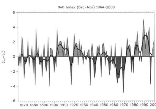
Abstract. This paper aims to provide a comprehensive review of previous studies and concepts concerning the North Atlantic Oscillation. The North Atlantic Oscillation (NAO) and its recent homologue, the Arctic Oscillation/Northern Hemisphere annular mode (AO/NAM), are the most prominent modes of variability in the Northern Hemisphere winter climate. The NAO teleconnection is characterised by a meridional displacement of atmospheric mass over the North Atlantic area. Its state is usually expressed by the standardised air pressure difference between the Azores High and the Iceland Low. This NAO index is a measure of the strength of the westerly flow (positive with strong westerlies, and vice versa). Together with the El Niño/Southern Oscillation (ENSO) phenomenon, the NAO is a major source of seasonal to interdecadal variability in the global atmosphere. On interannual and shorter time scales, the NAO dynamics can be explained as a purely internal mode of variability of the atmospheric circulation. Interdecadal variability may be influenced, however, by ocean and sea-ice processes.
Keywords:atmospheric circulation, climate, flow, North Atlantic Oscillation
Abbreviations:AMO – Atlantic Multidecadal Oscillation; AO/NAM – Arctic Oscillation (synonym to Northern Hemisphere annular mode, NAM); AOGCM – Atmosphere-Ocean General Circulation Model; AOI – Arctic Oscillation Index; CCA – Canonical Correlation Analysis; ECMWF – European Centre for Medium-Range Weather Forecasts; ENSO – El Niño/Southern Oscillation; EOF – Empir- ical Orthogonal Function; EU – Eurasian Pattern; GA – Greenland Above; GB – Greenland Below;
GC – Gyre Circulation; GCM – Global Circulation Model; GHG – Greenhouse Gas; GIN Seas – Greenland-Iceland-Norwegian Seas; GR – Gridded NAOI by Luterbacher et al. (1999; 2001a); GSA – Great Salinity Anomaly; HU – NAO by Hurrell (1995a); ITCZ – Intertropical Convergence Zone;
JO – NAOI by Jones et al. (1997); LO – Lorenz index (Lorenz 1951); MFT – Multiresolution Fourier Transform; NAC – North Atlantic Current; NAO – North Atlantic Oscillation; NAOI – North Atlantic Oscillation Index; NCEP/NCAR – National Center for Environmental Prediction/National Center for Atmospheric Research; NG – Temperature Norway Greenland (Wallace 2000); NH – Northern Hemisphere; PC – Subpolar SLP principal component; PCA – Principal Component Analysis; PNA – Pacific North American Pattern; PNJ – Polar Night Jet; PJO – Polar-night Jet Oscillation; QBO – Quasi Biennial Oscillation or Tropical Biennial Oscillation; RO – normalised NAOI by Rogers (1984); SH – Southern Hemisphere; SIC – Sea Ice Concentration; SLP – Sea Level Pressure; SST – Sea Surface Temperature; SVD – Singular Value Decomposition; TAV – Tropical Atlantic Vari- ability; TDS – Transpolar Drift Stream; THC – Thermohaline Circulation; TW – AOI according to Thompson and Wallace (1998); WA – Western Atlantic; WB – Walker and Bliss NAOI (1932).
Surveys in Geophysics 22: 321–382, 2001.
© 2001Kluwer Academic Publishers. Printed in the Netherlands.
1. Introduction
Everyone living in Europe knows that different winters have different characterist- ics. For example, the winters between 1975 and 1995 were generally mild and there was little snow in Central Europe, whereas in the 1960s winters were often cold and dry like 1963 and sometimes large amounts of snow were observed (Wanner et al., 1997; Uppenbrink, 1999). Meteorologists would say that air temperatures and snowfall in both cases were related to the atmospheric circulation over the North Atlantic–European sector. A long lasting weather situation can at most characterise a whole winter, but what makes mild or severe winters tend to occur in succession?
Some weather situations might occur over some years more frequently than others might, and then the opposite could be the case in other periods. This question is not only important for understanding climate but also raises the hope of being able to make seasonal forecasts.
One such mode that comes out of many climate statistics is often called the North Atlantic Oscillation (NAO; we will go into more detail about the concur- rent modes and the ongoing debate in the next Section). The NAO describes a large-scale meridional vacillation in atmospheric mass between the North Atlantic regions of the subtropical anticyclone near the Azores and the subpolar low pres- sure system near Iceland. It is a major source of seasonal to interdecadal variability in the worldwide atmospheric circulation (Hurrell, 1995a) and represents the most important “teleconnection” (some authors prefer the term “anomaly pattern” in this context; Wallace and Gutzler, 1981; Kushnir and Wallace, 1989) of the North Atlantic-European area (Hurrell and van Loon, 1997; Kapala et al., 1998), where it is most pronounced in winter. The measure for the state of the NAO, the North Atlantic Oscillation Index (NAOI) is widely used as a general indicator for the strength of the westerlies over the eastern North Atlantic and western Europe and most importantly for winter climate in Europe (Hurrell and van Loon, 1997; Wan- ner et al., 1997; WMO, 1998). In fact, the NAOI is highly correlated with a large variety of atmosphere-related environmental variables, mainly during the winter season (see Dickson et al., 2000 and Souriau and Yiou, 2001, for nice overviews).
The NAO is a descriptive summary, and consequently its precise definition de-
pends on the statistical approach used. Unfortunately, a uniquely defined NAOI
does not exist, nor is there a unique spatial pattern. However, the NAO is not only
the result of statistical considerations. What is behind the statistics, what is behind
the complex NAO dynamics? Is it simply the dynamical expression of the land-sea
distribution and orography of the Northern Hemisphere (NH) that inevitably has to
come out from any circulation statistics? Or is it the expression of time-dependent
processes, or both, a result of spatio-temporal considerations? Is the NAOI varying
randomly or is it controlled on certain time scales? Does the NAO respond to for-
cings applied by volcanic eruptions, changes in the solar activity, greenhouse gases,
or just by anomalous ocean temperatures? There is no single conceptual framework
to what exactly controls the NAO. There are alternative views; a situation which
characterises the current debate. A pattern that is closely related to the NAO, the Arctic Oscillation (AO) or Northern Hemisphere annular mode (NAM; Thompson and Wallace, 1998; 2001; Wallace, 2000) has recently received much attention. It is defined as the leading EOF of the monthly sea level pressure (SLP) fields north of 20
◦N weighted by area. The AO has large similarities to the NAO with respect to its spatial pattern and their index series are highly correlated (more details will be given in Chapter 6). NAO and AO describe the same phenomenon, but lead to different dynamical interpretations (Wallace, 2000). In a recent paper, Delworth and Dixon (2000) denote the NAO as the regional representation of the largest changes in midlatitudes associated with the AO, occurring in the Atlantic sector.
In this contribution, we would like to present both views. However, since there is the danger to be judged from the use of an acronym, we want to make clear that we use the acronym NAO whenever the phenomenon is referred to (for historical reasons) and make the distinction between NAO and AO/NAM when discussing the dynamical concepts.
The NAO has received a lot of attention in the climate research community espe- cially in recent years, and even more so with the proposition of the AO/NAM. The NAO-AO/NAM issue rivals the El Niño/Southern Oscillation in terms of its signi- ficance for understanding global climate variability (Wallace, 2000). Researchers from other fields have started to be interested in this phenomenon, and it appears more and more in the media. Despite the lack of a unifying concept, many detailed studies have been published and some new dynamical ideas have been developed in the last years (for an overview see Greatbach, 2000).
This paper aims to inform a broader scientific community and even interested non-specialists about the complex NAO-AO/NAM phenomenon. Section 2 aims to give an overview about the concept and the dynamics of the NAO or related modes. The history of its discovery and research is described in Section 3. This part of the article is designed to be understandable also for the above mentioned non-specialists. The North Atlantic Oscillation dynamics, including their spatial representation, are described in the Sections 4 and 5 by including not only obser- vational but also theoretical and modeling studies. Section 6 presents the statistical analysis of mainly two time series of NAO indices. This part also comprises a diagnostic study of the state of the NAO since AD 1659, including a spectral analysis. Section 7 deals with the simulated future trends of the North Atlantic and Arctic Oscillations (NAO and AO/NAM) in climate models and the projected changes for the future. Conclusions from the point of view of the researcher and consequences for our understanding of climate are given in chapter 8.
2. North Atlantic Oscillation: The Phenomenon
Circulation modes such as the NAO are found by decomposing the spatio-temporal
variability of atmospheric variables into spatial patterns on one hand, and time
series that describe the strength of the patterns on the other. The decomposition can be based entirely on statistical methods. This is the case of the AO. It can also be based on a priori knowledge, such as the predominance of the Azores High and the Icelandic Low for weather and climate in Europe. This is the case for the NAO. It should be noted that these are not the only centres of action relevant for European weather and climate. Other modes like the Eastern Atlantic and the Eurasian Pattern (EU) are also important (see e.g., Barnston and Livezey, 1987;
Cayan 1992b and Luterbacher et al., 1999).
Before entering the discussion about the concepts and the dynamical back- ground, we would like to start the paper with a short description of the spatial manifestation of the NAO pattern in the SLP distribution and to look at the regional impact, i.e., the spatial pattern of the relation of other relevant climate variables (temperature, precipitation) to the NAO.
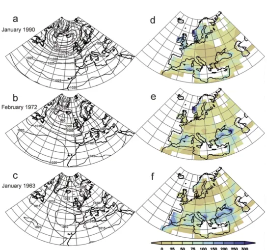
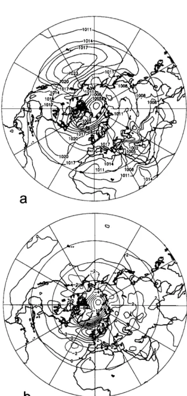
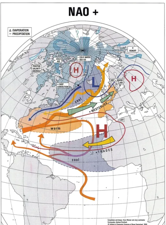
The SLP distribution over the North Atlantic for the positive NAO mode (NAO + ) has a well developed Icelandic Low and Azores High, associated with stronger westerlies over the eastern North Atlantic and the European continent. Fig- ure 1a shows an example of a month (January 1990) with a strong pressure gradient between Iceland and the Azores, thus a positive NAOI. In the negative NAO mode (NAO − ), an example is shown in Figure 1b (February 1972), the Icelandic Low and the Azores High are rather weak, thus giving rise to reduced westerlies over the eastern North Atlantic. Note, however, that in the negative NAO mode, the pressure distribution is not necessarily reversed. There is still an Icelandic Low and an Azores High, but weaker than normal. Complete reversals with higher pressure over Iceland region than over the Azores region in a monthly average (extremely negative NAOI) occur very rarely but are particularly important. They share a remarkable part of the interdecadal variability of the surface air temperature in the North Atlantic sector (Moses et al., 1987). An example of a reversal in SLP is given in Figure 1c (January 1963) which was associated with a strong easterly flow over the eastern North Atlantic. Other winter months with typical reversals were January 1881 and January 1918.
The positive and negative phases of the NAO mode are accompanied by differ-
ent spatial patterns of precipitation. In the positive phase (Figure 1d), precipitation
is high over Scotland and southwestern Norway. In contrast, in the case of the
reversal (Figure 1f), high amounts of precipitation were observed in the Medi-
terranean area and the Black Sea (see also Hurrell and van Loon, 1997). Both
phases of the NAO can be described with one anomaly pattern of different sign
that has to be added to the mean SLP distribution and the strength of which can
be measured. Section 3, from a historical point of view and Section 6 will go
into more details concerning the different North Atlantic Oscillation indices and
related indices. Note that the NAOIs are usually defined as the normalised pressure
difference between two stations in the vicinity of the Azores High and the Icelandic
Low. The Arctic Oscillation index is defined as the first principal component time
series of the SLP fields north of 20
◦N. There is not only a positive or negative
Figure 1.Monthly mean sea level pressure (a–c, hPa) and precipitation (d–f, mm) for January 1990, February 1972, and January 1963, respectively. Sea level pressure data are from NCEP/NCAR Reanalysis Data (Kalnay et al., 1996; Kistler et al., 2001), precipitation data are from Hulme (1992).
mode of the NAO, but also “everything” in between. That means, the NAO has rather a continuum of possible states than a finite set of regimes, and a bimodality in the different NAOI series is not determinable (see Section 6).
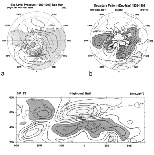
When regressing SLP time series at each grid point upon a NAOI, the resulting field of regression coefficients (often called “amplitude or regression pattern” to distinguish it from the “correlation pattern”, i.e., the pattern of the correlation coef- ficients at each grid point) is no longer influenced by the mean SLP distribution.
The dipole character of the NAO appears very clearly. This is shown in Figure 2a
for a time series of winter mean SLP values (December to March) using the winter
NAOI of Hurrell (1995a) from 1935 to 1999 (based on Lisbon and Stykkisholmur
station pressure). The area of negative coefficients extends over the northern North
Atlantic, the Arctic Basin and North Siberia and a zonally structured area of op-
posite sign appears over the central North Atlantic and the Mediterranean area. The
Figure 2.Spatial pattern of the NAO and its influence on temperature and precipitation, defined for winter means (December to March); (a) SPL anomalies projected on the NAOI (Hurrell, in Visbeck et al., 1998). (b) Observed surface temperature change associated with a one standard deviation of the NAOI. The regression coefficient was computed for the winters of 1935–1996. Dark (light) shad- ing indicates positive (negative) changes (Hurrell and van Loon, 1997). (c) Precipitation anomalies associated with the NAO; E−P (Evaporation minus Precipitation) is plotted, computed as a residual of the atmospheric moisture budget using ECMWF global analyses, for high NAO index minus low index winters (after Hurrell, 1995).
highest pressure changes with changing NAOI are found over the Denmark Strait and the area east and west of the Iberian Peninsula, and not exactly over Iceland and the Azores.
Amplitude or correlation patterns for the different NAOIs and concurrent pat-
terns look rather similar. The most important difference is that in the Arctic
Oscillation amplitude pattern of SLP, the southern centre of action is more zonally
elongated towards Europe and North America and the Northern Pacific centre of action is stronger, which gives a more “annular” appearance. Yet, also the AO shows a predominance of the Atlantic-European region (Deser, 2000; Ambaum et al., 2001). The subtle differences in the spatial patterns of the various indices are not shown here, the reader is referred to the figures in the papers of Thompson and Wallace (1998; 2000; 2001), Cullen et al. (2000), Deser (2000), Wallace (2000) and Ambaum et al. (2001).
By regression of the hemispheric temperature and precipitation fields on the same NAOI, we distinguish clear but different spatial patterns. The observed tem- perature change associated with one standard deviation change of the NAOI (Figure 2b) shows that the NAO has a dominant influence on the wintertime temperatures of the NH, especially in the area between North America and Eurasia (Hurrell and van Loon, 1997). Southwest of Iceland and east of the Gulf of Bothnia the changes are clearly higher than 1
◦C per one standard deviation. Similar to the temperature changes, the precipitation anomalies related to NAOI changes (Figure 2c) show the classical seesaw between west Greenland and west Scandinavia (van Loon and Rogers, 1978; Hurrell, 1995a). This seesaw or pendulum is also well known from the winter temperatures between western Greenland and northwest Europe (van Loon and Rogers, 1978). The pendulum swings between “Greenland Above”
(GA) and “Greenland Below” (GB) normal winter temperatures. During the GB- mode (an expression of the positive NAO phase), temperatures in the Greenland region and across southern Europe and the Middle East tend to be below average, but above average in the eastern United States and across northern Europe (Walker and Bliss, 1932; van Loon and Rogers, 1978; Stephenson et al., 2000). The pos- itive NAO phase is also associated with above-normal precipitation over northern Europe (including Iceland) and Scandinavia and below-normal precipitation over southern and central Europe as well as Northwest Africa (see Figure 1). Oppos- ite patterns of temperature and precipitation anomalies are typically found during strong negative NAO phases in the GA-mode (van Loon and Rogers, 1978). In addition, the wintertime precipitation anomalies depict the north-south gradients between Greenland and the Bermuda Islands, as well as between Scandinavia and the Mediterranean Sea.
The regional climate impact of the NAO has been subject to a vast number of detailed studies. The interested reader is referred to these studies, dealing with the correlation between the NAO and the regional or continental distribution of important variables such as temperature, precipitation, or sea-ice (e.g., van Loon and Rogers, 1978; Lamb and Peppler, 1987; Hurrell, 1995a; Hurrell, 1996; Mal- berg and Bökens, 1997; Rodó et al., 1997; Wanner et al., 1997; Kapala et al., 1998; Koslowski and Glaser, 1999; Osborn et al., 1999; Pozo-Vásquez et al., 2001;
Slonosky and Yiou, 2001).
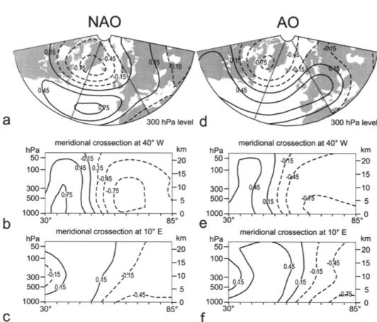
The NAO has distinct upper tropospheric features. Figures 3a–c show the correl-
ations between the monthly 3-dimensional geopotential height anomaly field and a
NAOI (based on station data from Ponta Delgada and Reykjavik; see Luterbacher
Figure 3.Correlations between monthly geopotential height anomalies and the NAOI (a–c) and the AOI (d–f), respectively, for the months November to April 1958 to 1997 (n = 240). (a, d): maps of the correlations at 300 hPa. (b, e): meridional cross-section at 40◦W. (c, f): meridional cross-section at 10◦E. Geopotential height data are from the NCEP/NCAR reanalysis data set (Kalnay et al., 1996;
Kistler et al., 2001), AOI from Thompson and Wallace (1998). The NAOI is based on Ponta Delgada and Reykjavik station pressure (for details see Brönnimann et al., 2000).
et al., 1999) for the winter months (November to April) from 1958 to 1997. Since in this case the winter months were pooled in a sample rather than averaged, the long term mean annual cycle of geopotential height was removed prior to analysis.
Correlations are displayed at the 300 hPa level (Figure 3a) and in two meridional cross-sections at 40
◦W (Figure 3b, representing a cut through the centres of action of the NAO) and at 10
◦E (Figure 3c, downwind on the European continent).
The correlation pattern at 300 hPa (Figure 3a) differs from the surface patterns
only in some details. The upper tropospheric structures of the NAO are displaced
slightly westward. Apart from the dipole-like structure, a third feature appears at
subtropical latitudes (Figures 3a and c), for which there is no corresponding surface
signature, as previously noted by Appenzeller et al. (2000). The meridional cross-
sections reveal a close to vertical structure over the North Atlantic but a northward
displacement with height over Europe.
Figures 3d–f present the correlations of geopotential height with the Arctic Os- cillation Index (AOI). In the upper troposphere and stratosphere, AO and NAO show similar structures over the North Atlantic, but geopotential height fields reveal clearly higher correlations to the AOI than to the NAOI over Europe and America (see also Thompson and Wallace, 2000). The correlations between geo- potential height over the North Atlantic and the wintertime NAOI and even more so with the AOI are significant up to the 100 hPa and 50 hPa levels; thus the NAO/AO signal encompasses the whole troposphere and lower stratosphere of this region.
This association is strongest in winter, which consequently, is often called the
“active season”. In January and February, the NAO signal was even detected in the mesopause winds at ∼ 95 km height (Jacobi and Beckmann, 1999).
The clear signal in the stratosphere merits further attention since stratosphere- troposphere coupling is relevant for many climate processes, such as solar and volcanic climate forcing, internal system dynamics such as sudden stratospheric warming, El Niño/Southern Oscillation (ENSO) and Quasi Biennial Oscillation (QBO; Perlwitz and Graf, 1995). It might also be useful for the understanding of long-term stratospheric ozone variability (Appenzeller et al., 2000; Brönnimann et al., 2000). Leading modes of stratosphere-troposphere coupled variability in the NH extracted from geopotential height fields by means of Singular Value Decom- position (SVD; Baldwin et al., 1994) or Canonical Correlation Analysis (CCA;
Perlwitz and Graf, 1995) reveal a stratospheric pattern that describes strength and position of the polar vortex and a tropospheric pattern that resembles the NAO, but which exhibits a more zonally symmetric structure. As mentioned above, this pat- tern was later identified as “Arctic Oscillation” by Thompson and Wallace (1998;
2000; 2001) and interpreted as the surface signature of modulations in strength of the polar vortex aloft. Correlating the SLP monthly anomalies of the NH with the leading Empirical Orthogonal Function (EOF) of the 50 hPa level gives essentially the same pattern (Deser, 2000). Thus, note that the NAO and AO/NAM are coupled with the polar vortex in the stratosphere. Over the Atlantic, a pattern similar to the NAO is also found in the difference in 1000 hPa geopotential height composites between westerly and easterly QBO phases (Baldwin et al., 2001). Section 4 will go more into the details with respect to stratosphere-troposphere coupling.
To conclude this Section on the spatial aspects of the North Atlantic climate
oscillations, we note that the spatial pattern of the NAO is a pronounced dipole-like
pressure anomaly over the North Atlantic and has associated patterns of anomalies
of temperature and precipitation over Europe, the Atlantic and even the eastern
United States. The AO pattern is very similar. However, it encompasses the entire
extratropical hemisphere, but with the largest signal over the Atlantic sector. The
signal of both, NAO and AO is not confined to the surface but reaches up to the
middle atmosphere.
3. History and Concepts
3.1. H
ISTORICAL REVIEW OF PREVIOUS NAO-
RELATED STUDIESIn this chapter, the history of research on NAO-related topics is reviewed. It can be seen that many of the earlier views and concepts still resound in current research on NAO and AO. For other aspects of the early work, the reader is referred to the original papers and to the overviews given by Wallace (2000) and Stephenson et al. (2000).
The occurrence of periods with mild and severe winters, of course, was clearly noted by people many centuries ago. The first written evidence related to the “NAO phenomenon” dates back to at least the eighteenth century. As described in van Loon and Rogers (1978), the missionary Hans Egede Saabye made the following observations in a diary which he kept in Greenland from 1770–1778: “In Green- land, all winters are severe, yet they are not alike. The Danes have noticed that when the winter in Denmark was severe, as we perceive it, the winter in Greenland in its manner was mild, and conversely”. In his book on “Historie von Grönland”, published in 1765, D. Crantz wrote about the opposition of winters in the two regions. Traders and missionaries visiting Greenland were aware of this “telecon- nection” between Danish and Greenland climate, although they did not have the necessary measurements for further scientific investigation.
In the nineteenth century, when more data became available, climatologists
began to study the spatial characteristics of winter temperature. Dove (1839; 1841)
investigated some 60 temperature series of up to 40 year length from the NH and
noted that anomalies vary more pronounced between East and West than between
North and South. He noted a double opposition of the monthly or seasonal tem-
perature anomalies of northern Europe with respect to both, North America and
Siberia, and found this to be in agreement with the statement by Hans Egede
Saabye. Hann (1890) then illustrated the seesaw by using 42 years of monthly mean
temperatures from Jakobshavn on the west coast of Greenland (69
◦N, 51
◦W) and
Vienna (48
◦N, 16
◦E) in Austria. Later studies used Oslo, Norway (60
◦N, 11
◦E)
instead of Vienna. One trigger for the work of meteorologists at that time was
the experience of some anomalously cold winters in Europe such as the winter of
1879/80. Teisserenc de Bort (1883) started to study the positions of large pressure
centres (he defined the term “centres of action”) during anomalous winters. He dis-
tinguished five types of anomalous winters according to the position of the Azores
High and the Russian High and to some extent also the Icelandic Low. He suggested
that surface influences (such as Eurasian snow cover) were responsible for these
displacements. Petterson (1890) and Meinardus (1898) investigated the influence
of the Gulf Stream on weather and climate in Western Europe. They suggested
that interannual fluctuations in the Gulf Stream system could be responsible for
anomalous winters, and they noted that these fluctuations could affect the weather
in western Iceland and Greenland in the opposite way than in Europe.
The focus of most meteorologists and climatologists at that time, however, was more concerned with describing the phenomena rather than understanding its un- derlying processes. Around the turn of the century, meteorologists started to think about seasonal forecasts and used a more statistical approach to study weather and climate. Hildebrandsson (1897) plotted pressure series from different sites and found a distinct inverse relation between the pressure at Iceland and the Azores. He also noted that series from the Azores and Siberia ran “parallel”, whereas Alaska and Siberia showed an opposite behaviour. An impetus to this kind of “statistical”
climatology was the concept of correlation, which was invented in 1877 by Francis Galton, but first published in 1888 (cf. Johnson and Katz, 1998). Walker (1909) and Exner (1913) were some of the first to apply this technique in climatology.
While the focus of Walker’s work was the prediction of the Indian Monsoon and the flooding of the Nile, Exner’s interest was mainly the extratropical NH. He published a map of the correlation between the monthly pressure anomalies at the North Pole (approximated by the mean of three series from Greenland, northern Norway, and Northern Siberia, respectively) and some 50 sites in the NH (Figure 4a). He pointed to the annular appearance of the pattern and the strong signature in the North Atlantic and Mediterranean areas. In fact, his correlation pattern is similar to the one of the AO (Wallace, 2000). On the other hand, his work remained statistical and did not really address the physical processes behind the polar vortex.
Figure 4b shows Exner’s map of correlations of pressure anomalies between Stykkisholmur and some 70 sites (Exner, 1924). This pattern resembles more the classical NAO pattern. Walker (1923) expanded his earlier statistical work to in- clude also the North Atlantic area and addressed the “Iceland-Azores Oscillation”.
In his milestone paper (Walker, 1924), he described three modes which dominate world weather and introduced the terms North Atlantic Oscillation, North Pacific Oscillation (the two Northern Oscillations) and Southern Oscillation. He vaguely related the NAO to the Gulf Stream and the sea-ice dynamics in the North Atlantic, but he was sceptical about periodicities of 2 and 4.5 years of the sea-ice extent off Iceland and Iceland pressure that were discussed by other scientists at that time. Part of Walker’s genius in isolating dominant modes was the way he expertly
“rejected” spurious correlations using significance testing.
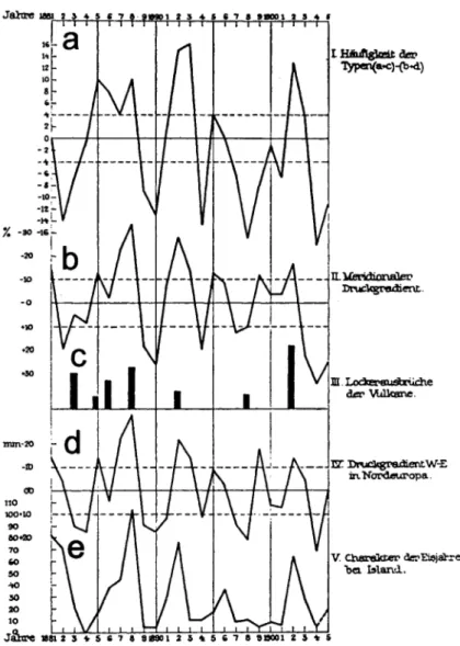
In the same year, Defant (1924) published a study on the monthly SLP anomaly
fields over the North Atlantic. He distinguished two pairs (four types) of anomalies,
where the first pair (83% of all months) corresponds to the NAO-pattern and the
second pair to a strong anomaly at 55
◦N and a weak opposite anomaly between
10
◦and 30
◦N. By subjectively attributing to each month an anomaly type and a
strength and applying a weighting procedure he was able to draw annual time series
(Figure 5). He related this to the anomalies of the zonally averaged meridional
pressure gradient over the Atlantic, volcanic eruptions, the zonal pressure gradient
between Northern Europe and the northern North Atlantic, and the sea ice extent
off Iceland. He considered these variations to be internal oscillations of the climate
system of 3–5 years periodicity that were disturbed by volcanic eruptions. Defant
Figure 4.(a) Map of the correlation between monthly anomalies of “polar pressure” (average of three stations in northern Greenland, northern Norway, and northern Siberia, respectively) and pressure at around 50 sites of the Northern Hemisphere from 1887 to 1906 (from Exner, 1913). (b) Map of the correlation between monthly anomalies of pressure at Stykkisholmur and pressure at about 70 sites for winter months (September to March) from 1887 to 1916 (from Exner, 1924).
Figure 5.Time series from 1881 to 1905 of different variables from the study of Defant (1924). (a) Defant’s circulation index, where negative values correspond to a positive NAO; (b) percent anomaly of the pressure gradient between 60◦to 70◦N and 25◦to 35◦N, averaged from 10◦to 60◦W; (c) index of volcanic eruptions; (d) pressure difference between Northern Europe (0◦to 40◦E, 60◦to 75◦N) and the North Atlantic between 60◦and 70◦N (in mm Hg); (e) duration of sea ice cover off Iceland (in eights of a month).
(1924) also pointed to possible relations between the North Atlantic climate and the
“heat engine” of the tropical Atlantic, taking up older, speculative ideas of Shaw (1905) and Hann (1906).
Walker’s concept of the NAO became very popular among contemporary met-
eorologists and created the need for a quantitative measure of the strength of the
NAO. Walker and Bliss (1932) constructed the first NAOI in a rather complex,
iterative procedure involving seven time series of temperature and SLP data from Europe and North America, by using the following formula:
P
Vienna+ T
Bodö+ T
Stornoway+ 0.7P
Bermuda− P
Stykkisholmur− P
Ivigtut− 0.7T
Godthaab+ 0.7(T
Hatteras+ T
Washington)/2.
P stands for air pressure and T for air temperature averaged over the winter period December to February. The individual series were standardised to have standard deviations of √
20, and the weights were discovered iteratively. It is interesting to note that the series of Azores pressure was found to be a bad NAOI predictor and was excluded in the procedure. According to Wallace (2000), Walker and Bliss (1932) procedure can be considered to be an iterative approximation to Principal Component Analysis (PCA).
Further descriptive studies were published in the 1930s on the temperature seesaw between Northern Europe and Greenland (Angström, 1935; Loewe, 1937).
At about the same time, along with a change-over from a descriptive, statistical view of climatology and meteorology to an explanatory, dynamical approach, new concepts on climate variability in the Atlantic-European region were developed. A number of theoretically motivated studies about the interaction of the zonal circu- lation and pressure centres were published by a group of leading meteorologists such as Rossby, Willett, Namias, Lorenz and others (Lorenz, 1967). Although the improvement of forecasts motivated the background for this research, these authors focussed more on the dynamics of the system governing equations.
Rossby et al. (1939) studied the structure and dynamics of the planetary waves in the presence of disturbances and deduced an influence of the strength of the zonal circulation on the temporal behaviour of the quasi-stationary centres of ac- tion. To address the hemispheric zonal circulation in the presence of embedded eddy disturbances, they introduced a “zonal index” defined as the zonally averaged difference between SLP at 55
◦N and 35
◦N. For Rossby, it was clear that this was a measure for the strength of the polar vortex in the free atmosphere to the north.
Later, Rossby and Willet (1948) intensified their studies on the polar vortex and addressed the issue of stratosphere-troposphere coupling. Rossby’s zonal index be- came popular for a certain time, and climatological studies of the zonal circulation were performed. Namias (1950), with a clear focus towards the improvement of forecasts, recognised the importance of latitudinal shifts in the zonal mean zonal wind. Lorenz (1950) studied the variability of the zonal mean circulation and the oscillations in the distribution of atmospheric mass. He introduced a new index, defined as the zonal mean meridional pressure gradient at 55
◦N. In fact, there were many different zonal indices used at that time (Kutzbach, 1970), however, none of them became popular (see Wallace, 2000, for a more detailed discussion).
Building on the impressive study by Helland-Hansen and Nansen (1920),
Bjerknes (1964) reviewed ocean-atmosphere-interaction in relation to North At-
lantic climate variability. He pointed to the important role of the atmosphere for the
heat exchange and discussed in detail trends and anomalies in Atlantic sea surface
temperatures (SST) as induced by atmospheric stresses and oceanic circulation.
Bjerknes (1964) used the pressure difference between Iceland and the Azores as a simple measure of westerly flow strength. This is in fact a simple North At- lantic Oscillation index, although Bjerknes preferred the term “zonal index”. A noteworthy element of this work is the dynamical analysis of past climate variab- ility (largely based on studies done by Lamb and Johnson, 1959; 1961). Bjerknes presented ideas on the extraordinary situation in the North Atlantic from 1780 to 1820 with respect to air–sea interaction.
A much used descriptive statistical approach for isolating maximum variance patterns in the large scale circulation is the PCA of the SLP field. Although some work had been done in the 1950s (e.g., Lorenz, 1951), it was mainly Kutzbach (1970) who pioneered the use of this method for studying large scale circulation an- omalies. PCA gives patterns and corresponding time series (principal components) of the patterns, which can be related to other time series. Many later studies have successfully used the same approach for SLP as well as for geopotential height fields: e.g., Trenberth and Paolino (1980), Wallace and Gutzler (1981), Barnston and Livezey (1987), Kushnir and Wallace (1989), Cayan (1992a, b), Thompson and Wallace (1998) and Volodin and Galin (1999). The first principal component pattern in winter looks relatively similar in all studies. The differences are mainly due to the selection, density and weighting of grid-points as well as due to rotated or non-rotated principal components.
The intention of these studies of the 1980s was to find the dominant modes of the low-frequency atmospheric circulation. Wallace and Gutzler (1981) pointed to the zonally symmetric, global-scale seesaw between polar and temperate latitudes in the SLP, as well as to the more regional-scale pattern resembling the so-called Pacific North American (PNA) and Western Atlantic (WA) pressure patterns at mid-tropospheric levels. By applying similar techniques to a 700 hPa level geopo- tential height data set, Barnston and Livezey (1987) showed that the NAO is the only low-frequency circulation pattern which is found in every month of the year.
Other studies in the 1970s re-examined the winter temperature see-saw between Greenland and Northern Europe (van Loon and Rogers, 1978; Rogers and van Loon, 1979; Meehl and van Loon, 1979). They found significant correlations between circulation and SSTs and investigated the teleconnections with the Pacific region and with the tropical climate system. These studies significantly “shaped”
the current concept of the NAO as a large-scale climate mode in the North Atlantic region with important impacts in European climate. The new efforts in the field of North Atlantic climate variability in the 1970s and 1980s were partly triggered by the dominance of the positive NAO phase at that time and by the increasing requests for seasonal climate forecasts. This view is represented by Lamb and Peppler (1987) who outlined the main concept of NAO and applied it to a regional climate problem, namely to the interannual variation of Moroccan precipitation.
The idea of a two point NAOI capturing the two quasi-permanent pressure centres
of the North Atlantic, the Azores High and Icelandic Low, was re-introduced by
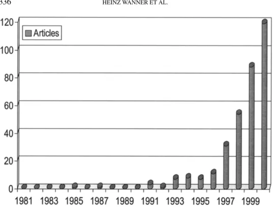
Figure 6.Bar-plot showing the increasing number of published articles containing the expression
“North Atlantic Oscillation” either in the title or in the abstract during the period 1981 and 2000.
Source: web of science bibliographic database.
Rogers (1984). He defined the NAOI as the difference in the standardised SLP series from Ponta Delgada, Azores minus Reykjavik, Iceland.
In the beginning of the 1990s, the NAO was studied in more detail in the light of
ocean-atmosphere interactions. The NAOI was related to interdecadal variabilities
of latent and sensible heat flux anomalies of the North Atlantic and the oceanic
circulation (Cayan, 1992a, b; Deser and Blackmon, 1993; Kushnir, 1994). At about
the same time, climate modellers began to search and study the NAO in their model
simulated climates (Delworth et al., 1993). In the 1990s, the number of scientific
papers on the NAO grew very rapidly. Figure 6 shows the number of all articles
with the expression “North Atlantic Oscillation” in either the title or the abstracts
between 1981 and 2000. The interest in NAO appeared at the beginning of 1980s
(in 1984 Rogers published his NAO paper). In the following decade, the tremend-
ous increase – a small NAO-boom – of the number of published papers indicates
the growing interest on this topic, especially after the publication of Hurrell in
1995 (Hurrell 1995a). In 2000, have been published 119 papers about NAO itself,
its influence and correlation with other phenomena.
Hurrell (1995a) investigated the influence of the NAO on temperature and pressure variability over the European continent on the interannual to decadal timescale. Since pressure observations at Azores go back only about one century, Hurrell defined a new NAOI as the difference between the standardised station pressure series of Lisbon minus Stykkisholmur, Iceland. This index has become the most commonly used NAOI in climate research. Jones et al. (1997) further ex- tended an instrumental NAOI back to 1821 by using station pressure observations from Gibraltar and the Reykjavik area. For studying low frequency atmospheric variability over the Atlantic-European area, it is necessary to extend the NAOI even further back into the pre-instrumental period of the Little Ice Age. There- fore, a focus of current research is to reconstruct NAOIs using early instrumental pressure, temperature and precipitation station series and environmental proxy and documentary proxy data (White et al. 1996; Cook et al., 1998; 2001; Appenzeller et al., 1998; Luterbacher, et al., 1999; Cullen et al., 2000; Luterbacher et al., 2001a, among others). Section 6 presents our new, highly resolved monthly NAOI reconstruction back to AD 1659.
The modern debate concerning the NAO-AO/NAM gave rise to a more intense reflection also on the definition of NAO. First of all, the questions were raised whether it makes sense or not just to use a two-point index with fixed locations. On the one hand, a two-point definition is simple and easy to apply. On the other hand it is obvious that more sophisticated statistical techniques allow a better spatio- temporal description of the phenomenon. By using EOF techniques, Barnston and Livezey (1987) and Glowienka-Hense (1990) have already indicated that the two nodes of the North Atlantic dipole displace with changing seasons. Wanner et al.
(1997) and Portis et al. (2001) have studied this seasonality of the NAO. They showed that both nodes migrate westward during summer. Recently, Cullen et al.
(2000) and Luterbacher (2001a) tried to optimise the NAO reconstructions by using multiproxy data (see also Section 6.1). Finally, Slonosky and Yiou (2001) tried to evade the problem of the seasonal shift of the pressure centres by using two different two-point indices (Ponta Delgada – Reykjavik in summer and Gibraltar – Reykjavik in winter).
To complete the picture, it must be mentioned that Schlesinger and Ramankutty (1994) as well as Schlesinger et al. (2000) described an oscillation in the global climate system with a period of 65–70 years. Kerr (2000), by discussing the cli- mate swing between a cold and warm phase in the North Atlantic, called this phenomenon Atlantic Multidecadal Oscillation (AMO).
What does the history of research on North Atlantic climate variability tell us?
Firstly, different motivations can be distinguished, recurring from time to time:
diagnostic analysis of recent climate variability, interest in the processes governing
the climate system and its internal variability, the hope to be able to do seasonal
forecasts and – a relatively new motivation – the analysis of low-frequency natural
(as opposed to anthropogenic) climate variability using proxies and climate mod-
els. Secondly, the concepts of NAO and AO are closely linked in a historical view.
They did not develop separately from each other, nor is the NAO concept a “histor- ical accident” (Thompson and Wallace, 1998; Deser, 2000) and the AO concept a new invention. Both concepts have roots in the historical debate. Thirdly, ever since Hildebrandson and Walker, a weak association between the North Atlantic and the Pacific SLP was admitted but the North Atlantic area was mostly considered to dominate the NH teleconnections. Fourthly, the underlying dynamical explanations for the NAO-AO oscillations still provide a major challenge to be addressed for understanding of climate variability.
3.2. N
ORTH ATLANTIC OSCILLATION VERSUS ARCTIC OSCILLATION OR NORTHERN HEMISPHERIC ANNULAR MODEIn their EOF analysis, Slonosky et al. (1997) pointed to the association between sea ice cover and air pressure variations. They remarked on the barotropic nature of this oscillation. Thompson and Wallace (1998; 2000; 2001) determined the leading EOF of monthly SLP fields north of 20
◦N weighted by area. The pattern they found has striking resemblances to the NAO in the Atlantic sector, but is zonally more symmetric with one centre of action over the Arctic region and an annular structure with opposite sign at mid-latitudes. They called this pattern “Arctic Os- cillation” in order to emphasise its Arctic aspect and to show its resemblance to the dominant “Antarctic Oscillation” mode of the extratropical Southern Hemisphere (SH) (Thompson et al., 2000). More recently, it is now referred to as the Northern Hemisphere annular mode (NAM; Wallace, 2000).
What distinguishes the AO/NAM from the NAO? It is not so much the spatial pattern but the interpretation. In the NAO framework, the pressure distribution (mainly at the surface level) over the Atlantic, i.e., the Azores High and the Icelandic Low, is the main actor. The zonal mean signal evident in statistics is merely an imprint of the Atlantic. As a consequence, possible driving factors are looked for in the North Atlantic region that involve the ocean and sea-ice dynamics.
In the more general AO view, the main actor is the zonal circulation and the At- lantic signal is a regional modification of the primary zonal signal. The equivalent barotropic structure and the dynamics of the higher atmosphere, namely the polar vortex appears as a more tempting forcing in this framework. According to Deser (2000), the annular appearance of the AO is caused by the Arctic centre of action, while there is no coordinated behaviour of the Atlantic and Pacific centres of action.
Ambaum et al. (2001) show that the NAO reflects the correlations between the
surface pressure variability at all of its centres of action whereas this is not the case
for the AO. Monthly mean SLP in the Pacific and Atlantic are not significantly
correlated yet both locations have large loading values in the AO pattern. The only
significant correlation between centres of action in the AO pattern is between the
Iceland and the Azores (Ambaum et al., 2001). In this sense, the authors conclude
that the latter is not a covariance structure and state the possible interpretation that
the AO is a non-local artefact of PCA.
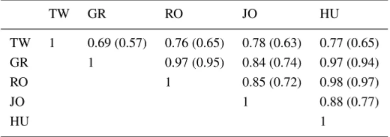
To learn more about the differences between NAO and AO, it could be worth- while to study the anomaly during a month where the different NAOIs and the AOI were far apart. Figure 7 shows the SLP field (raw in Figure 7a and anom- alies in Figure 7b) from the 1961 to 1990 climatology of such a month (August 1976). The Hurrell-NAOI (Lisbon minus Stykkisholmur) was − 2.7, a gridded NAOI (65
◦N/20
◦W–60
◦N/15
◦W minus 40
◦N/30
◦W–35
◦N/25
◦W) was − 4.5, the Jones-NAOI (Gibraltar minus Reykjavik) was − 3.5, and the NAOI based on Ponta Delgada and Reykjavik (Luterbacher et al., 1999) was − 4.2. While there are already considerable discrepancies within the different NAOIs for this particular month, they nevertheless all agree that the meridional pressure gradient over the Atlantic was strongly reduced. In contrast, the AOI has a clearly positive value ( + 0.9). How can this be explained? If one considers the NAO as a regional phe- nomenon of the North Atlantic and the AO as a hemispheric zonal pattern, one would assume a major anomaly in a region other than the North Atlantic. However, as can be seen in Figure 7b, this is not the case. There is the signature of a strong polar vortex, but there is also a negative anomaly at the Azores region. The most remarkable feature is the pronounced high pressure anomaly over the North Sea, from Ireland to Norway.
The North Atlantic or the Arctic Oscillation are currently open to debate on interpretation (Deser, 2000; Wallace, 2000; Ambaum et al., 2001). On a long term, we are certain that this debate is likely to prove fruitful for our understanding of the climate system. However, in the current discussion the question has to be asked:
Is the NAO obsolete? We do not believe that the NAO is obsolete. The AO is a statistical construct, resulting from an EOF analysis (Ambaum et al., 2001). If it were to be connected to one distinct mechanism, then the assumption would be that the effect of different processes on the SLP anomaly field would be strictly in- dependent (orthogonal), which is not reasonable. The AOI is a statistically derived measure. Mainly because of its size, it explains more of the northern hemispheric temperature variability than the NAOI. The AOI captures the largest fraction of the variability of the SLP distribution and has stronger trends correlated with those in many environmental phenomena than does the NAOI. But is the AO therefore closer to the “driving mechanisms” than the NAO? Not necessarily. In contrast to Wallace (2000), we do not believe that one has to decide between the two.
Rather, the AO concept has opened the eyes of many researchers not to neglect
the upper troposphere and stratosphere and to consider the hemispheric-scale zonal
circulation and the energetics and dynamics behind it, whereas the NAO concept
has made scientists think about ocean-atmosphere interaction and search causes for
low-frequency climate variability.
Figure 7.The extratropical northern hemispheric SLP distribution. (a) raw data, (b) anomaly with respect to 1961 to 1990, in August 1976.
4. Dynamical Aspects of the NAO
This Section will discuss different possible mechanisms for the NAO. Firstly, the question is asked whether the clue could be found simply within the atmosphere or not. Secondly, the influence of the ocean, including the important dynamical processes related to ocean-atmosphere interactions within the Atlantic region is addressed. Aspects concerning the influence of the thermohaline circulation (THC) and the SST variability in the tropical Atlantic area are also discussed in this Sub- section. A third Subsection, centred on the freshwater problem in the subpolar and polar area, brings the polar sea ice, the evaporation to precipitation relationship and the run off from the huge northern landmasses to the Arctic Ocean basin into play.
The pioneering paper on SST-SLP-interactions was published by Bjerknes (1964).
By analysing SST and SLP anomalies, he came to the conclusion that interannual SST variability is mainly driven by changes in the heat flux from the atmosphere, but that ocean dynamics (especially heat transport) play a major role in controlling SSTs on interdecadal timescales.
In general, it is important to emphasise that many of the discussed problems are still very controversial, and open to many debates. Therefore, the crucial question about how far the NAO is an expression of a climate regime (Palmer, 1999), which itself is the result of a single climate forcing, or a certain mix or cocktail of different (natural and/or anthropogenic) forcing factors, is not tackled in this review article.
4.1. T
HE NAO,
A PURELY ATMOSPHERIC PHENOMENON?
The question arises whether the NAO could be a natural unforced atmospheric phenomenon or not. James and James (1989) found a long-term mode being able to create low-frequency variability, which is exclusively based on non-linear feed- backs within the atmosphere. Furthermore, Barnett (1985) and Marshall et al.
(1997) showed that it is possible to reproduce NAO-like fluctuations with atmo- spheric General Circulation Models (GCM), which are forced with temporally non-varying SSTs.
The observational preoccupation with North Atlantic weather and climate pro- vokes the old question as to whether the existence and the spatial arrangement of the NAO is to some extent an aggregated average of atmospheric synoptic behaviour consisting of east-northeast moving low pressure systems within the quasistationary wave in the lee of the Rocky Mountains and North America.
From the viewpoint of the NAO being a regional manifestation of the AO, the
planetary-wave signature embedded in the AO is induced by horizontal temperature
advection as a consequence of the zonal mean flow perturbation and the strong
local sources and sinks of heat, i.e., land-sea contrasts (Thompson and Wallace,
1998; 2000; 2001). In this context, it would be especially interesting to estimate
the dynamical influence of Greenland, for example in two numerical experiments
with and without considering the dynamical effects of the Greenland land mass
(K. Fraedrich, pers. communication). Furthermore, Hurrell (1995b) as well as Limpasuvan and Hartmann (1999) discussed the role transient and stationary eddy fluxes play for the maintenance of the different phases of the NAO-AO/NAM phenomenon. De Weaver and Nigam (2000) showed that the interactions between the zonal-mean flow anomalies and the climatological eddies make the dominant contribution to the maintenance of the NAO stationary waves.
One hypothesis that is presently discussed relates to the coupling between tropo- spheric and stratospheric circulation. Perlwitz and Graf (1995) as well as Kodera et al. (1996; 1999) and a large number of recent references point to the statistical con- nection between the strength of the stratospheric winter vortex and the tropospheric circulation over the North Atlantic. During winters with an anomalously strong stratospheric polar vortex, the NAO tends to be in its positive phase. The key actors in this mechanism are vertically propagating planetary waves originating from the troposphere and the zonal circulation at the tropopause level and in the stratosphere.
At some altitude these waves break, their energy dissipates and interacts with the mean flow. Following Perlwitz and Graf (1995), the lower stratospheric zonal wind and its vertical shear, influence upward propagation of planetary waves.
It is generally assumed that the strong westerly vortex in winter provides a waveguide for efficient upward propagation of tropospheric waves and therefore, an association between the stratosphere and the troposphere (“active season”). Fol- lowing Kodera and Kuroda (2000), the circulation can be forced in an AO-like way by downward propagation of zonal-mean zonal wind anomalies from the strato- sphere (typically in February, March) as well as by tropospheric waves (in early winter). The slow oscillation of the zonal-mean zonal wind in the stratosphere, the Polar-night Jet Oscillation (PJO) acts as a preconditioner and feedback. Kodera et al. (1999) also point to the interesting fact that, prior to the early 1970s, the NAO and Polar Night Jet (PNJ) indices varies almost independently, while recently they exhibit a similar variability.
Stratosphere-troposphere coupling is not restricted to short time scales. Perlwitz et al. (2000) studied the dynamics of the polar vortex in a long-term integration of a climate model and found two quasi-stable climate modes that can be described as a weak vortex and a strong vortex state. Both modes are related to different stratosphere–troposphere coupling mechanisms. The climate of the second half of the twentieth century, in this framework, showed stronger similarities to the weak vortex state.
The coupling mechanisms between the stratosphere and the troposphere offer
a platform for possible explanations of stratospheric controls on climate (includ-
ing NAO): QBO, solar cycle (Labitzke and van Loon, 1995), explosive volcanism
(Robock and Mao, 1992; Robock, 2000), ozone depletion and Greenhouse Gas
(GHG) induced global warming (Graf et al., 1998). Although it seems that the
atmosphere reacts in an AO-like way to some of these forcings, no final agreement
is reached as to what extent the stratosphere is actively controlling the long-term
behaviour of the NAO or AO (Baldwin and Dunkerton, 1999; Kuroda and Kodera,
1999; Thompson and Wallace, 2000; 2001; Thompson et al., 2000). Other scient- ists, however, do not believe in a stratospheric control of climate variability. Despite the more and more detailed picture we have of the statistical relations between stratospheric and tropospheric circulation, the most fundamental question remains unsolved: What is the direction of cause and effect and what is the feedback (see also Deser, 2000)?
4.2. O
N THE NAO DYNAMICS WITHIN THE NORTH ATLANTIC BASINAccording to the previous Subsection, one could argue that dynamical coupling with ocean and sea-ice would not be necessary to understand NAO dynamics.
Based on the findings by Bjerknes (1964) and on progress of knowledge related to the ENSO phenomenon, one has to consider dynamical coupling, especially on higher time scales. In contrast to the ENSO, which is a rather zonally arranged tropical phenomenon, the NAO system reaches from the tropical Atlantic Ocean to the polar basin with its sea-ice system. Its spatial extent is clearly smaller, and it must also be influenced by global processes outside the Atlantic area (Hurrell, 1996). This is one important reason for the complexity of the NAO and its dy- namics. We are therefore still far from having a consensus about the processes being responsible for the spatio-temporal NAO variability observed on different time scales, namely in the interdecadal range.
We first try to give, in the following Subsections, a short overview on pos- sible processes relevant for the generation of the NAO centred system variability within the North Atlantic Ocean, including the tropical Atlantic and the northern polar basin. We are not able to discuss extensively all the relevant processes being responsible for the generation of short to long term variability of the coupled ocean–sea-ice–atmosphere system in the Atlantic area. We consciously do not split the Subsections related to different time scales or between modelling and observations. We rather try to differentiate between a few dynamical phenomena or processes, which are important for the NAO dynamics, and therefore linked to specific regions.
4.2.1. NAO Related Atmospheric Forcing of the Ocean
If we follow Bjerknes’ (1964) concept of the time scale dependency of North
Atlantic air–sea interaction, we have to consider one way interactions between
atmosphere and ocean first, and then to look at complex coupled modes being
relevant for NAO. On interannual time scales, observational results demonstrate
that atmospheric anomalies might be able to force the variations in the ocean by
anomalous heat fluxes and surface mixing (Wallace et al., 1990; Zorita et al.,
1992). Hasselmann (1976) and Frankignoul and Hasselmann (1977) were able
to explain this active role of the atmosphere with the framework of a stochastic
climate model. In this model, weather noise, usually representing white spectra, is
integrated by the much slower reacting ocean, leading to spectra that are essentially
red down to frequencies where the system is stabilised by some internal feedback mechanisms. Later, Frankignoul et al. (1997) have extended the stochastic climate model to decadal time-scales. However, Stephenson et al. (2000) showed that the power spectrum of the NAO has increasingly more power at the low frequen- cies than expected from red noise, because of long-range dependence in the time series. Häkkinen (1999), based on a 43-year ocean model simulation (1951–93), showed that the meridional overturning cell and heat transport must be driven by the NAO related heat flux. Tsimplis and Josey (2001) found that the strengthening of the NAO from the 1960s to the 1990s explains a significant proportion of the reduction in Mediterranean Sea level over this period. The link arises from the combined effects of atmospheric pressure anomalies and changes in evaporation and precipitation.
In a recent study, Eden and Jung (2000) studied how the North Atlantic circula- tion responds to a forcing by the NAO on interdecadal time scales. They found that the observed and modelled developments of interdecadal SST anomalies during the periods 1915–1939 and 1960–1984 against the local damping influence from the NAO can be traced back to the lagged response (10–20 years) of the North Atlantic THC and the subpolar gyre strength to interdecadal variability of the NAO. This aspect has to be further discussed when looking at coupled modes. In conclusion, the NAO influences the Atlantic Ocean by inducing substantial changes in sur- face wind patterns, thereby altering the heat and freshwater exchange at the ocean surface, and influencing the thermohaline and horizontal gyres circulations (GC) (Hurrell et al., 2001).
4.2.2. Oceanic Forcing of the North Atlantic Atmosphere and NAO
The question how North Atlantic SSTs can influence the atmosphere and therefore also the NAO structure and dynamics is a pressing one. Frankignoul (1985) was able to demonstrate that atmospheric forced SST anomalies are damped by the turbulent surface heat fluxes, thereby influencing the atmospheric boundary layer.
Several authors looked at imprints of the upper ocean structure on atmospheric
circulation in winter or spring (e.g., Ratcliffe and Murray, 1970; Palmer and Sun,
1985). Together with Barnston and Livezey (1987), Peng and Mysak (1993) as
well as Peng et al. (1995), Palmer and Sun (1985) have shown that strongly an-
omalous warm SSTs near the coast of Newfoundland are significantly related to
atmospheric circulation anomalies, indicating a meridional pattern with positive
SLP anomalies over the North Atlantic (that is to say in the lee of the warm pool)
and negative values over north-western Europe. Czaja and Frankignoul (1999) have
further demonstrated that significant anomalies of the atmospheric circulation are
related to previous North Atlantic SST anomalies. For instance, a signal over the
northwest Labrador Sea in late spring is associated with the dominant mode of
SST variability during the preceding winter, and a NAO-like signal in early winter
is connected to SST anomalies east of Newfoundland and in the eastern subtropical
North Atlantic during the preceding summer.
Rodwell et al. (1999) as well as Mehta et al. (2000) used long time series of SSTs and sea-ice cover to force an ensemble of Atmosphere–Ocean General Circulation Model (AOGCM) integrations with the aim to examine the predictab- ility of the winter NAO and AO. They found that the modelled ensemble mean NAO indices correlate much better with the observed NAO indices than a typical individual integration. Rodwell et al. (1999) argue that the SST characteristics are “communicated” to the atmosphere through evaporation, precipitation and at- mospheric heating processes leading to changes in temperature, precipitation and storminess over Europe. However, Bretherton and Battisti (2000) used a simple model to explain the findings by Rodwell et al. (1999) and Mehta et al. (2000) as due to the artificial way in which such atmosphere models are forced by the ocean. They forced a linear model atmosphere/ocean interaction by high-frequency atmospheric stochastic variability and demonstrated, despite the hindcast skill, that the useful predictability, associated with midlatitude SST anomalies, is limited to one or two seasons.
By using the University of California atmospheric GCM, Robertson et al.
(2000) investigated the influence of the Atlantic SST anomalies on the atmospheric circulation over the North Atlantic during winter. Among other results, they found that the interannual fluctuations in the simulated NAO were significantly correlated with SST anomalies over the tropical and subtropical South Atlantic.
4.2.3. Dynamics of the Tropical and Subtropical Atlantic and Their Relation to NAO
During the last few years, the relations between the dynamics in the tropical and subtropical Atlantic and the NAO attached more importance. Nobre and Shukla (1996) and Black et al. (1999) have pointed to the covarying fluctuation between the Atlantic tropical SSTs and the trade winds. Together with Enfield and Mayer (1997), they showed that stronger than normal southeasterly trade winds in the SH are associated with negative SST anomalies and vice versa. Chang et al. (1997) demonstrated that the surface heat flux plays an active role in the tropical Atlantic.
Nevertheless, it is questionable whether the correlation in the decadal dipole – with a seesaw between negative SST anomalies in the SH and positive SST an- omalies north of the Intertropical Convergence Zone (ITCZ) – is highly significant or not (Houghton and Tourre, 1992). Several studies point to the possibility that the climate variability and the position of the ITCZ in the tropical Atlantic Ocean is sensitive to the cross-equatorial SST differences (Hastenrath and Heller, 1977;
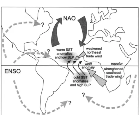
Folland et al., 1991; Servain, 1991; Chang et al., 1997). The dipole might also influence the rainfall over parts of South America (Moura and Shukla 1981) and the Sahel region (Lamb and Peppler, 1991). The variability of the NAO seems to be coupled to the northeasterly trades and the SSTs on the NH (see Figure 8).
Recently, George and Saunders (2001) demonstrated that the dominant mode of
wind speed variability in the wintertime tropical is represented by the NAO. They
also showed that that the winter NAOI determines monthly precipitation levels
Figure 8.Influence of ENSO and important mechanisms of Tropical Atlantic Variability (after Chang, adapted from Visbeck et al., 1998).