in the Last Glacial Maximum

in the Last Glacial Maximum

Determined by Atmospheric Model Simulations

I n a u g u r a l D i s s e r t a t i o n

zur

Erlangung des Doktorgrades

der Mathematisch-Naturwissenschaftlichen Fakultät der Universität zu Köln

vorgelegt von

Erik J. Schaffernicht

aus Köln

Prof. Dr. Joaquim G. Pinto, Karlsruher Institut für Technologie

Mündliche Prüfung am 24. Juli 2018

The Last Glacial Maximum (LGM) is a turning point of the Earth’s climate and the human dispersal.

Yet, the then prevailing atmosphere dynamics over Europe and the North Atlantic as well as the mineral dust cycle in Europe are not well understood. This dissertation improves understanding the LGM climate and its dust cycle. Based on global climate simulations, it compares the LGM climatologies, jet stream, Circulation Weather Types (CWTs), and Combined Empirical Orthogo- nal Functions (CEOFs) with their present analogues. The dust cycle was reconstructed for Europe based on statistic dynamic downscaling using CWT frequency-conform regional Weather Research and Forecasting Model (WRF) simulations for the LGM. Proxies and reanalyses served to evaluate all simulations; among them a comprehensive compilation of loess-based reconstructed mass ac- cumulation rates for the LGM. By comparing the simulated LGM depositions with these rates, a linkage was established between the LGM dust cycle and the present loess.

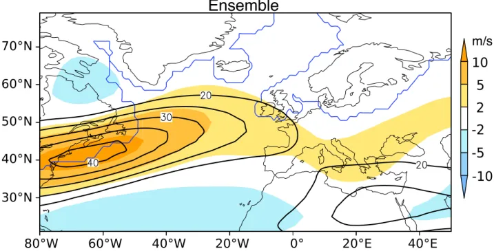
For the North Atlantic and Europe, the CEOFs suggest a lower LGM than present climate vari- ability. The jet stream was narrower and partly more than 10 m/s faster there. Possible subsequent jet stream paths ran over and along the Nordic Seas, eastwards along the onset of the Central Ger- man Uplands or over the Mediterranean. The North Atlantic Oscillation (NAO) was 50% stronger combined with a 6° wider (westward) Azores High. The latitude-deviating LGM temperatures indi- cate that the North Atlantic Current extended up to Norway. Precipitation reduced by more than 150 mm/yr over the proglacial European areas; including a reduction of more than 300 mm/yr over the North Sea Basin. Near the EIS coast, periods of precipitation and temperatures that ranged be- low their climatological average synchronized with above-average precipitation periods over the Azores; both likely correlating with a below-average NAO. Similarly, stronger EIS High periods correlated with reduced precipitation and temperatures in western and central Europe. Combined with strong dry northeast sector winds, they favored erosion along the proglacial areas. Consis- tently, more frequent southerlies, cyclones, and east sector winds occurred in central and eastern Europe. This agrees with katabatic winds and the EIS-induced blocking that shifted the storm tracks southward. In contrast to the present westerlies, east sector winds (36%) and cyclones (22%) dominated central Europe. The east sector winds dominated the dust transport from the proglacial EIS areas to central Europe. In particular over western Europe, cyclones and strong — yet rare — west sector winds contributed in addition to the dust transport. Most dust was emitted from the Alps-, Black Sea- and EIS-bounded area. Its emissions culminated in proglacial central Europe with peaks of more than 100 kg m^–2yr^–1. The LGM dust plumes mainly ran westwards along the EIS margin. The highest aeolian depositions covered West Poland, the German Bight, and the North German Plain (between 1 and 100 kg m^–2yr^–1). The significance of the east sector winds for the LGM is corroborated by the consistency of the simulated depositions and the mass accumula- tion rates reconstructed from more than 70 distinct loess sites across Europe.

Das letzte glaziale Maximum (LGM) ist ein Wendepunkt des Erdklimas und der Menschheitsaus- breitung. Dessen ungeachtet ist das Verständnis für die damalige europäische und nordatlantische Atmosphärendynamik sowie den Mineralstaubzyklus in Europa wenig ausgeprägt. Diese Disser- tation trägt zu einem besseren Verständnis beider bei. Basierend auf globalen Klimasimulationen werden die Klimatologien, der Jetstream, die Zirkulationswetterarten (CWTs) und die kombinierten empirischen Orthogonalfunktionen (CEOFs) des LGMs und der Gegenwart miteinander verglichen.

Zudem wird der Staubzyklus in Europa rekonstruiert mittels statistisch dynamischem Downsca- ling, welches CWT-Frequenz-konforme, regionale Weather Research and Forecasting (WRF) Mo- dellsimulationen nutzt. Unabhängige Referenzen für die Simulationsergebnisse bieten Reanalysen und Proxies. Im Rahmen Letzterer wurden ca. 100 lössbasierte Masse-Akkumulationsraten zusam- mengestellt. Deren Vergleich mit den simulierten Raten setzt den LGM-Staubzyklus in Beziehung zum gegenwärtigen Löss.

Für Europa und den Nordatlantik suggerieren die CEOFs eine geringere Klimavariabilität als heute. Der Jetstream war dort schmaler und teilweise mehr als 10 m/s schneller; mögliche Strö- mungspfade verliefen vor der Küste des eurasischen Eisschildes (EIS), ostwärts über den deut- schen Mittelgebirgen oder über dem Mittelmeer. Die Nordatlantische Oszillation (NAO) war 50%

stärker verbunden mit einem 6° westwärts ausgedehnteren Azorenhoch. Der Nordatlantikstrom reichte gemäß Breitengrad-abweichender Temperaturen bis nach Norwegen. Niederschläge fielen über Europas proglazialen Gebieten um mehr als 150 mm/a geringer aus; über dem Nordseebe- cken um mehr als 300 mm/a. Unterdurchschnittliche Niederschläge und Temperaturen über dem arktisnahen Atlantik und dem westlichen EIS sychronisierten mit überdurchschnittlichen Nieder- schlägen über den Azoren; wahrscheinlich korrelierend mit einer unterdurchschnittlichen NAO.

Phasen eines stärkeren EIS-Hochs gingen einher mit Niederschlags- und Temperaturrückgängen in Europa. Verbunden mit starken, trockenen Nordostsektorwinden begünstigten diese Rückgänge die Erosion der proglazialen Gebiete. Konsistent dazu traten häufigere Südwinde, Zyklonen und Ostsektorwinde über Mittel- und Osteuropa auf. Dazu passen die katabatischen Winde und das EIS-erzeugte Blocking, das die Sturmzugbahnen südwärts verschob. In Mitteleuropa überwiegten während des LGMs Zyklonen (22%) und Ostsektorwinde (36%). Die Ostsektorwinde dominierten den Staubtransport von den proglazialen EIS-Gebieten nach Mitteleuropa. Besonders über Westeu- ropa trugen auch Zyklonen und starke — aber seltene — Westsektorwinde zum Staubtransport bei.

Die stärksten Staubemissionen stammten von dem durch Alpen, Schwarzmeer und EIS begrenzten Gebiet. Dessen Raten gipfelten im proglazialen Mitteleuropa in vereinzelt mehr als 100 kg m^–2a^–1. Auftretende Staubwolken zogen hauptsächlich westwärts entlang des EIS-Rands. Die größten äo- lischen Sedimentationsraten (zwischen 1 und 100 kg m^–2a^–1) traten in Westpolen, der norddeut- schen Ebene und der Deutschen Bucht auf. Die Bedeutung der Ostsektorwinde wird durch die Konsistenz der für das LGM simulierten Ablagerungs- und der von mehr als 70 verschiedenen Lössfundstellen rekonstruierten Masse-Akkumulationsraten bestätigt.

Abstract 3

Zusammenfassung 4

Contents 5

1 Introduction 8

1.1 Motivation . . . . 8

1.2 The Past Climate is a Key to Respect our Future . . . . 9

1.3 Importance and effects of the Last Glacial Maximum for our Ancestors . . . 10

1.4 Glacial Dust Cycle, Climate Proxies, and Present Loess . . . 10

1.5 Linkage between the Glacial Dust Cycle and the Current Loess . . . 13

1.6 Goal and Methods . . . 15

2 The Last Glacial Maximum 16 2.1 Earth’s orbit triggered the Last Glacial Maximum . . . 16

2.2 Sea level, Ice sheets, and Lakes . . . 17

2.3 Temperature distribution . . . 18

2.4 Greenhouse gas concentrations during the LGM and until today . . . 19

2.5 Biosphere . . . 21

3 Climate and Proxy Data 23 3.1 Reanalyses and Global Climate Model Simulations . . . 23

3.2 Boundary Conditions for Regional Climate Simulations . . . 24

3.3 Climate Archives and Proxies . . . 24

4 Climatologies of the European and Atlantic Atmosphere 28 4.1 Introduction . . . 28

4.2 Hypotheses . . . 29

4.3 Methods . . . 29

4.4 Results and Discussion . . . 30

4.5 Conclusions . . . 43

5 Atmospheric Variability beyond Climatologies 45 5.1 Introduction . . . 45

5.2 Hypotheses . . . 46

5.3 Methods — Combined Empirical Orthogonal Functions . . . 47

5.4 Results and Discussion . . . 48

5.5 Conclusions . . . 67

6 Dominant Eastern Sector Winds over Europe 70

6.1 Introduction . . . 70

6.2 Hypotheses . . . 71

6.3 Methods — Circulation Weather Types . . . 72

6.4 Results and Discussion . . . 74

6.5 Conclusions . . . 88

7 Linkage of the European Dust Cycle and Loess Records 89 7.1 Introduction . . . 89

7.2 Hypothesis on the Glacial European Dust Cycle . . . 93

7.3 Methods — Statistic Dynamic Downscaling . . . 94

7.4 Results and Discussions . . . 98

7.4.1 Prevailing Eastern Sector Winds and Cyclones over Central Europe . . . 98

7.4.2 Major Erosion from the Fringes of the Eurasian Ice Sheet . . . 104

7.4.3 Dust Emission to Deposition Comparison within Europe . . . 110

7.4.4 Consistency of Simulated Dust Depositions and Loess Accumulation Rates . 113 7.4.5 Intra-Annual Distribution of Episodes . . . 139

7.4.6 Seasonally resolved Atmospheric Circulation and Dust Distribution . . . 146

7.4.7 Static LGM Boundary Conditions for Regional Dust Simulations . . . 148

7.5 Limitations . . . 155

8 Conclusions 159 8.1 Climatology of the Last Glacial Maximum . . . 159

8.2 Subclimatological Atmospheric Patterns . . . 160

8.3 Dominant Eastern Sector Winds over Central and Eastern Europe . . . 162

8.4 Linkage of the European Dust Cycle and the Loess records . . . 162

9 References 164 10 Abbreviations, Acronyms, Physical Units 187 11 List of Figures 190 12 Acknowledgments 193 13 Supplementary 195 13.1 Legal Statements . . . 195

13.2 Erklärung zur Dissertation . . . 196

13.3 Teilpublikation . . . 196

acronyms that are not expanded on their first occurrence.

1 Introduction

1.1 Motivation

The paleo climate and environment affected the migration of Homo sapiensto and within Europe during the last 200 000 years^1,2. Yet, robust knowledge on their migratory conditions and routes lacks^3–6: How, where, and under which conditions were settlements chosen in Europe? For ex- ample, settlements disintegrated repeatedly on the Iberian Peninsula⁷, possibly due to Heinrich Events⁸; yet, a well-established theory is still missing. Also, the central European settlement hia- tus^7,9,10related to the Last Glacial Maximum (LGM, 21 000±3 000 years ago^11,12) is not completely understood and contradictory assumptions have been published: either the western European pop- ulation withdrew to refugia in southern France and on the Iberian Peninsula at that time^10,13; or the European population expanded considerably at 23 ka ago according to mitochondrial DNA analy- ses^14,15. In this case, it possibly affected vulnerable fauna¹⁶.

To improve the understanding of human migration to and within Europe, the Collaborative Re- search Centre 806 (CRC806) ‘Our Way to Europe’ was established⁷consisting of three phases. The research leading to this dissertation formed part of its second phase, during which the CRC806 en- compassed the following collaborating disciplines (marked arethose, which closely relate to data, methods or findings of this dissertation): physical geography,sedimentology,geology, geomorphol- ogy, speleology, archaeology, anthropology, palynology, paleobotany, and meteorology including mineral dust modeling. Within the CRC806 framework, this dissertation implements an interdis- ciplinary research approach and perspective.

Almost all these disciplines focus on fieldwork. Yet, the scope of fieldwork is usually limited to addressing one or a few sites; each extending between some meters up to a few kilometers at maximum. Sampling, excavation or core drilling is rarely carried out at high spatial resolution for areas of a 100 km² or larger. Therefore, it often remains unanswerable whether fieldwork-based reconstructions represent more than a local site-specific finding — in particular when focusing on fieldwork only. Fieldwork alone can either not or only fragmentarily provide the surrounding three dimensional spatial context on regional to continental scales.

This dissertation provides this missing context. It focuses on the LGM climate including the reconstruction of the mineral dust cycle for the LGM. Its findings base on analyzing global^17–20 and performing regional climate-dust simulations to reconstruct the dust cycle. These findings are evaluated by relating them to climate proxies. This referencing advances the interpretation of the fieldwork results and the climate simulations, as it establishes the complementary paleoclimatic context to fieldwork.

This dissertation establishes a more complete multidisciplinary understanding of the Earth’s past climate; its analyses and reconstructions serve to understand the interaction between the atmo-, oceano-, cryo-, bio-, and pedosphere. Their relevance is not limited to the CRC806; on the contrary, they show connections that also serve soil scientists, atmospheric chemists, and cli- matologists. Its climate analyses enable to assess the regional significance and to establish the supra-regional understanding of fieldwork results.

1.2 The Past Climate is a Key to Respect our Future

In this dissertation, the LGM is analyzed and compared to the present climate. The LGM represents a fundamentally different state of the Earth’s climate (Sec. 2). However, it is not the only time when a global temperature trend resulted in a fundamentally different climate. Since the industrialization and more vigorous since the 1950s, the humans force global warming, which affects the Earth’s climate drastically^21–23. Though the current human-induced global warming trend is inverse to the cooling trend during the LGM onset, both trends modify the Earth system dynamics and severely affect the genera^24–26. However, in contrast to the pace of the temperature trend leading to the LGM, the driving pace of the human-induced global warming is much faster than any previous well-understood global temperature trend during the existence ofHomo sapiens^21–23.

During the Earth’s past, similar or even faster climate changes were only caused by major as- teroid impacts followed by mass extinctions²⁷. So far, severe mass extinctions on Earth have been rare: only five in the last 540 million years²⁴. After the most recent impact 65 million years ago 70% of the Earth’s marine invertebrate species vanished; 50% of all genera perished^27,28. Despite this being published in 1980, and despite the serious number of species that already died out in the last decades, almost all humans, who cause the ongoing greenhouse gas emissions, decide—by sticking to their behavior—to continue loosing biodiversity^24–26,28. The first human-induced mass extinction is very likely, as it has already begun²⁹.

The survival of species has depended and will continue to depend on feedback and tipping points that control, balance or torpedo the Earth’s climate system — depending on the immanent non- linear dynamics of this system. Their understanding is crucial to be aware of present and upcoming global warming hazards^23,30–32. The accomplishment of our near future depends critically on both, the best possible understanding of the non-linear climate dynamics, and our swift action now to stop any additional human-induced global warming^21–23. In addition, our rapid societal action is needed to mitigate the already inevitable and ever-increasing impact of the existing climate crisis.

This dissertation enhances knowledge of the climate dynamics and variability beyond the aver- age quasi-stationary state that lasted for at least the last two to three millennia before industrializa- tion. The comparison of the LGM with this state emphasizes the different and thus characteristic dynamics and variability of each of them. Improving their understanding is crucial to recognize the changing patterns during the transient, globally warming climate today and in the near future.

1.3 Importance and effects of the Last Glacial Maximum for our Ancestors

In the Earth’s past climate, the LGM is the most recent turning point (Sec. 2). Although it offered new potential human habitats and migration routes, such as the narrowed Strait of Sicily, the dry Bosporus and northern Adriatic, the restriction by the atmosphere, the cryosphere, and their in- teractions with the pedosphere during the LGM dominated human mobility^33,34. As a result of the increased aridity³⁵, particular in central to eastern Europe^36–40, the pre-glacial biomes including their specific fauna deteriorated or shifted⁴⁰, thereby reducing their human carrying capacity.

The LGM reduced the European megafauna considerably¹⁶. The woolly mammoth and several other species disappeared across central Europe^10,41. The giant deer withdrew from western and central Europe¹⁰. Many other species withdrew to refugia⁴²; for example, reindeer remains dated to the LGM were mainly found south of 50°N indicating the southward retreat of the reindeer pop- ulation⁴¹. This exemplifies the effects of the LGM on the megafaunal range dynamics^40,41.

Phylogeographic patterns indicate isolated populations in southern European LGM climate refu- gia⁴². Mitochondrial DNA of pre-LGM bears evidences almost no such patterns. This presumably applies also to many European species⁴². It indicates the significant impact of the LGM climate on the fauna evolution⁴¹.

In Eurasia, the reindeer probably was the main human resource⁴¹. Its retreat presumably re- duced the human carrying capacity of northern central Europe during the LGM, which proba- bly reversed the human expansion, i.e. the decreasing human population withdrew to the glacial megafauna refugia. To interrelate how the varying human population density and climate af- fected the megafaunal species, an improved understanding of the LGM climate is needed¹⁶. This dissertation provides this by analyzing the LGM climate in Europe and over the North Atlantic (Sec. 4, 5, and 6) as well as by reconstructing the LGM environment with a particular focus on mineral dust (Sec. 7). Ultimately, the accomplished LGM climate analyses and dust cycle recon- struction pave the way for modeling the human mobility during the LGM.

1.4 Glacial Dust Cycle, Climate Proxies, and Present Loess

Despite the importance of the LGM in the Earth’s past climate, its regional atmospheric charac- teristics including the aeolian mineral dust cycle are not well known. For this cycle, the boundary layer winds and their directions are of particular importance. On the local scale, wind proxies en- able the reconstruction of the then prevailing surface wind directions. Yet, these reconstructions are often ambiguous and their extrapolation to regional or continental scales is controversial.

Many studies assume that westerlies continuously dominated Europe during the LGM similar to present-day westerlies^43–45. However, plenty of evidence exists for prevailing north and east sector winds during the LGM in Europe: Central and eastern European sediments indicate north sector winds⁴⁶. Easterlies are evidenced by several proxies across Europe: grain size records in northern central Europe⁴⁶, Eifel sediments⁴⁷, heavy minerals and carbonate peaks⁴⁸, Harz Foreland loess⁴⁹, and wind-polished rocks⁴⁵ in central Europe near the margin of the Eurasian ice sheet. Danish proxies in addition evidence southeasters⁴⁵. In Hungary and the Carpathian Basin, sediments evidence north sector winds, westerlies, and southeasters^46,50–52. Ukrainian sand deposits evidence north sector winds^46,52.

To evaluate these proxy-based, yet partly opposing wind direction reconstructions, and to over- come the absence of instrumental observations, the wind distribution in Europe during the LGM was analyzed in this dissertation based on global climate simulations. At the regional scale, the simulated pressure patterns were classified into Circulation Weather Types^53–55 (CWTs) . The GCM quality was assessed by comparing the CWT frequencies that result from their simulations for the recent climate with those resulting from reanalyses. Key characteristics of the regional wind distribution during the LGM were revealed by comparing the CWT frequencies calculated from the LGM simulation with those calculated from the simulations of the recent climate. Compiling the western, central, eastern, and southern European distributions establishes a pan-European refer- ence for the LGM wind system. This enables relating the distinct kinds of local wind proxies with the pan-European wind system and serves to reconstruct the LGM dust cycle for Europe by statis- tic dynamic downscaling.

The dominant LGM wind directions directly affected the aeolian mineral dust cycle in Europe at that time. This cycle is of particular interest because mineral dust is a core theme in Earth system science and climate sciences⁵⁶: For example, aeolian dust enhances or suppresses precipitation⁵⁷; it alters the radiation budget; its deposits evidence changing aridity⁵⁸ and paleo wind systems⁵⁹.

Compared to the present, reduced LGM wet depositions³⁵, the more vigorous atmospheric cir- culation, and stronger cyclones at the upper mid-latitudes^60,61 relate to the at least ten times greater dust loads during the LGM⁶². Over erodible areas, strong winds presumably transformed to dust storms hindering humans by reducing the visibility to zero⁶³. Increased aridity³⁵, severe cold^64–71, huge ice sheets^17,72,73, and the lower sea level^12,74–77led to more dust sources³⁵; many of them probably near the southern or eastern margin of the Eurasian ice sheet⁴⁴.

This dissertation improves the understanding of the high-resolved spatial distribution of dust emission rates by taking into account effects of vegetation, snow, ice, and soil moisture on the emissions. Although the LGM temperatures and greenhouse gas concentrations were lower than today⁷⁸, understanding how extreme aridity, strong winds, and steep topography affected aeolian erosion allows to improve the projections of erosion dynamics for the upcoming climate.

Dust is relevant to paleo sciences, as it is frequently found in all kinds of climate archives, which are the only in situ fragments for reconstructing the local paleoclimate. Some of these archives such as sediments and ice cores record in addition also regional and global paleoclimate properties.

Therefore, it is important to understand these archives in the best possible way. Yet, transforming climate archives to meaning- and insightful climate proxies is in some cases not at all, in most cases not well or not completely understood. Improvement is needed on extracting data and converting it to statements, understanding, and context — which corresponds to learning from the fragments of the ‘book’ written by nature at times far beyond the individual and societal memory.

In this dissertation climate proxies for the LGM are compared to simulation results for tem- perature, precipitation, and wind (Sec. 4, 5, and 6). The dissertation provides the complementary spatial context and reveals the unknown dynamics that explains the encountered patterns of, and the reconstructed values from the proxies. It reveals and establishes the linkage between the LGM dust cycle in Europe and one of its most important proxy — the loess.

Loess is particularly appropriate for validating spatially resolved dust simulations, because it is on land the most prominent, widely, and abundantly distributed dust deposition proxy in Europe;

it has been sampled and analyzed for decades⁷⁹. In Europe, loess covers large areas⁷⁹(Fig. 41); its creation began 75 kyr ago, followed by the enhanced built-up during the last glacial, and ended 15 kyr ago⁸⁰. In the eastern European history, the LGM represents the most substantial phase of loess accumulation⁸¹. Its thickest layers form the European loess belt at about 50°N. They extend from France to the eastern European Plain⁸², which stretches from Slovakia to the Caspian Moun- tains. This belt includes the large loess sheets of the southern proglacial EIS regions, which are optimal for studying the paleoclimate^79,83–85.

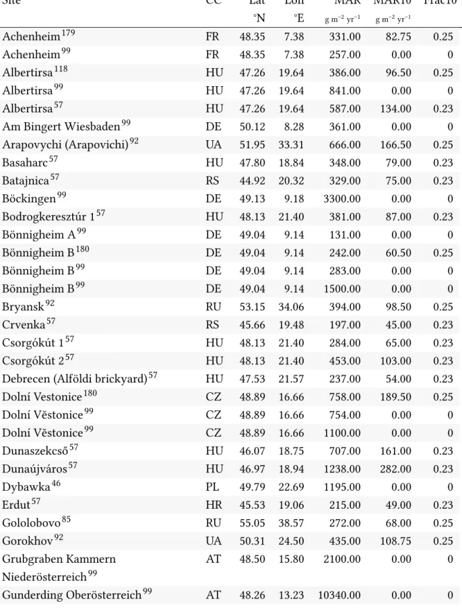
This dissertation contributes a concise, new, and otherwise missing overview (Tab. 1) of all (∼100) from loess for the LGM reconstructed mass accumulation rates (MARs) for the domain that was defined to reconstruct the dust cycle for the LGM. This state-of-the-art overview enables the quan- titative, independent, and spatially resolved verification of the simulated LGM dust deposition rates for Europe.

1.5 Linkage between the Glacial Dust Cycle and the Current Loess

Although most of the present-day loess-paleosol sites in Europe include a sequence that poten- tially originated from dust accumulations during the LGM, the linkage to their corresponding LGM dust sources is not well known. This has seriously compromised their value as climate proxies.

As large amounts of dust were transported during the LGM, it is particular important to establish this linkage for this period⁸⁰.

Laboratory analyses of European sediment samples are one attempt to restore this linkage. For the LGM, they result in European dust source locations up to the littoral of the Aral Sea⁸⁶: The Lower Rhine Embayment loess likely originated from sources further west⁸⁷. Central European sediments refer to sources south or southeast of the EIS, north or east of the Alps, and around the Carpathians46,57,88,89. The Carpathian loess refers to various sources⁴⁶. Aeolian contributions to the loess in the Lower Danube Basin come from the dry-fallen Black Sea littoral⁹⁰.

Drawbacks of the proxy-based reconstructed linkages are their dating dependence and, for some types of proxies, their dependence on assumptions on the past atmospheric circulation that do not necessarily apply homogeneously to all locations or past periods. In addition, these linkages are fragments of knowledge; they do not explain the atmospheric dust dynamics nor do they abstract from the individual sediment to the general context. To overcome these fieldwork-inherent short- comings, this dissertation contributes to reveals the linkage between the dust cycle during the LGM and the present-day loess distribution in Europe based on climate-dust simulations for Eu- rope (Sec. 7).

A few fieldwork-based studies of sediments offer a reconstruction of the dust transport di- rection(s) that caused the respective sediment: For the LGM, aeolian sediments in the Eifel evi- dence easterlies⁴⁷. For the Late Pleniglacial, proxies evidence westerlies and southwesters near the Polish-Ukrainian border⁴⁶, northerlies and northwesters in the Carpathian Basin⁴⁶, and north sector winds that transported dust and sand from the proglacial plains to Ukraine, Romania, and the eastern Carpathians^46,52. Serbian and Ukrainian loess sites evidence east sector winds^46,91. The central and eastern European loess partly originated from the Aral Sea implying dust-transporting easterlies and southeasters⁸⁶.

These proxy-inferred directions usually base solely on (a few) samples taken only from one site or sediment core. The resulting MARs and wind directions often vary considerably for neighbor- ing sites⁴⁶. Their temporal scope is generalized to long time spans such as the Late Pleniglacial, which itself consisted of distinct atmospheric circulation periods due to the varying Eurasian and Laurentide ice sheets⁶⁹. The reconstruction of the LGM wind dynamics and dust cycle exclusively from sediments is problematic because the samples do not contain any indicators to distinguish dust contributions of rare storms from those of the frequent wind directions⁴⁵.

These discrepancies and uncertainties of the dust proxies show the need for state-of-the-art pa- leo dust modeling, which is provided by this dissertation. The therefore accomplished climate- dust simulations serve to establish the linkage between the LGM dust cycle and the loess records.

They contribute to an improved understanding of the LGM dust cycle in Europe.

For glacial climates, only a few simulation-based studies have been published that researched on the mineral dust cycle43,44,92–98. Two of them^43,44 limited their domain to a sub-European re- gion during the Marine Isotope Stage 3. Due to their domain extent (8° latitude, 20°–40° longitude) and non LGM-compliant ice sheets^43,44, it is very unlikely that they approximate well the real dust cycle during the LGM in Europe⁶⁹. The deposition rates that are calculated for the LGM by the GCMs^92–98(between 1 and 100 g m^–2yr^–1) significantly underestimate the loess-based recon- structed MARs for Europe46,57,59,99.

This GCM deficiency to represent the real dust cycle during the LGM is corroborated by failing GCM dust simulations¹⁰⁰ for 1982 to 2005. These present-day dust simulations run by 23 GCMs systematically underestimate the dust emissions and transport that is obtained independently from fieldwork and satellite observations¹⁰⁰. These underestimated dust processes presumably result from the insufficient resolution, dust schemes, dust size and source distributions of the GCMs^35,100,101. In summary, up to now, GCMs fail to represent the dust cycle for both, the present and the LGM. As a consequence, both, appropriate global and regional climate-dust simulations are missing for Europe during the LGM.

This dissertation provides the more appropriate reconstruction of the dust cycle. It overcomes the existing discrepancy of fieldwork- and simulation-based rates for the LGM. To this aim, high-resolved regional climate-dust simulations were run using the WRF-Chem-LGM. The WRF-Chem-LGM is a version of the Weather Research and Forecasting Model coupled with Chemistry^102–105 (WRF-Chem) that was slightly upgraded for this purpose to respect the effects of a glacial environment on the dust emissions, and to consider LGM-specific boundary conditions (Sec. 7.3). The WRF-Chem-LGM simulations avoid several and reduce considerably the remaining deficiencies compared to the previous43,44,92–98 simulations by others. The LGM upgrade of the WRF-Chem takes into account glacial vegetation, topography, and dust sources. It hinders dust emissions proportionally to the areal fraction covered by snow or ice sheets.

It is unprecedented in the LGM climate-dust modeling to combine the online¹⁰² atmosphere- dust interaction, the high resolution over the whole European domain, and the dust cycle complete- ness. This completeness comprises the dust emissions by aerodynamic entrainment, saltation bom- bardment, and aggregate disintegration¹⁰⁶; the dust transport, the gravitational settling¹⁰², the dry and the wet deposition^102,107.

In contrast to most dust simulations^92,96,108, the performed WRF-Chem-LGM simulations are neither tuned nor otherwise manipulated towards any predefined outcome, which distinguishes the current approach from many others. The consistency of the fieldwork-based MARs46,57,59,99 and the simulated deposition rates shows the quality of the simulations contributed by this dissertation.

Independent findings provide a complementary perspective on my results and assess their rel- evance. These independent references comprise other simulations43,69,96–98,109–113, geomorpho- logical, biological, and geological climate proxies, such as marine sediments¹¹⁴, pollen^70,115–117, coleoptera⁷¹, sand deposits⁵², equilibrium line altitudes⁶⁶, as well as the spatial distribution and the rates of about a hundred local fieldwork-based reconstructed mass accumulations of loess sites in Europe (Sec. 7 and Tab. 1).

1.6 Goal and Methods

This dissertation creates the linkage between the mineral dust cycle during the LGM and the present-day loess deposits in Europe. To achieve this goal, a comprehensive understanding of the LGM climate dynamics and its differences to the present climate dynamics is sought. This encompasses the recognition of atmospheric patterns that dominated the LGM in contrast to the present climate. To accomplish this, the analyses based on different kinds of scientific data: first and foremost on climate and climate-dust simulations; for the verification of the simulations, the analyses also base on various climate and dust proxies, among others pollen^70,115–117, rocks⁴⁵, fossils⁷¹, marine sediment cores¹¹⁴, glacier equilibrium line altitudes⁶⁶, sand deposits^45,52, and loess46,57,85,92,99,118–125. The verification of the simulation-based dust depositions is facilitated by a comprehensive mass accumulation rate compilation based on loess deposits all across Europe (Tab. 1).

The pattern recognition includes the analysis of and the comparison between the LGM and the present climatologies for the principle variables of the atmosphere: pressure, temperature, and precipitation. It also includes the subclimatological decomposition of these variables using com- bined empirical orthogonal functions¹²⁶to understand the variables’ reciprocal dependency, feed- back, and interaction. The combined empirical orthogonal functions provide insights into the syn- chronous spatial atmosphere dynamics patterns generated by the variables’ interaction and their feedback to the remaining Earth system components and dynamics.

In addition to the effects of this reciprocal climate dynamics on the mineral dust cycle, the dust transport is determined by the prevailing winds. This is taken into account for Europe by classifying the daily simulation-based weather variability using the CWT analysis^36,53–55. This classification enables the statistic dynamic downscaling based reconstruction of the LGM dust cy- cle. This reconstruction requires regional episodic climate-dust simulations for the LGM. These were created by running a LGM-adapted version of the Weather Research and Forecasting Model coupled with Chemistry^102–105 (WRF-Chem). The domain boundaries of these simulations were driven by the LGM simulation of the Max‐Planck‐Institute Earth System Model^18–20,127(MPI-ESM).

The CWT-based dust simulations enable to establish the linkage between the current loess deposits and their LGM dust sources.

2 The Last Glacial Maximum

2.1 Earth’s orbit triggered the Last Glacial Maximum

The LGM (21 000±3 000 years ago^11,12) is a milestone of the Earth’s past climate. Within the Qua- ternary, it is the most recent major climatic turning point that marks the transition from the Pleis- tocene to the Holocene.

The astronomical theory of paleoclimate¹²⁸explains the onset of the Last Glacial by the favorable period of the Earth’s orbit and rotation. The superposition of the different cyclic variabilities that describe the configuration of the Earth towards the Sun limits the conditions to cyclic and discrete time slots that allow for glaciation. The dynamics of the Earth leads to a continuous realization of Earth Sun configurations that are different from their predecessor within the cyclic variability range. Thus, each realization of a successive configuration potentially leads to a change of the seasonal and latitudinal distribution of the Earth’s insolation.

During the Quaternary, ice ages began when successive low northern hemisphere insolation configurations prevailed¹²⁹, which enabled the growth and rise of vast northern hemispheric ice sheets during a few millennia. The mechanisms that allowed the onset of the Last Glacial can be reduced to three changes in the Earth’s orbit. The eccentricity 𝑒 of the Earth’s orbit varies during the 100 kyr cycle and determines the total amount of energy received by the Earth^128–130. The Earth’s axis inclination𝜀(obliquity or tilt) varies about 1.5° during the 41 kyr tilt cycle, which affects the latitudinal distribution of the incoming radiation, hence the seasonality⁷³. The spatial distribution and the seasonal pattern of the insolation depends on 𝜀 and 𝑒sin𝜔, with̄ 𝜔̄ as the longitude of the perihelion¹²⁸. The latter term describes the changing insolation due to the 21 kyr precession cycle, which takes into account the times of maximum and minimum Earth Sun distance combined with the effect of the changing insolation angle during the year.

Hence, the term 𝑒sin𝜔̄ describes the precession effects that modify the seasonal partitioning of the insolation. Thus, the superposition of both, 𝑒sin𝜔̄ and 𝜀, determines the Earth’s spatiotemporal surface distribution of the incoming energy. In accordance with this theory, the northern hemispheric boreal summer insolation density was lower than average during the onset of the Last Glacial. Moreover, mid-month and monthly mean insolation can explain long term climatic changes that have occurred during the Quaternary. Particularly, the mid August and the daily autumnal equinox insolation showed negative deviations about 20 kyr ago, coinciding with the LGM¹³¹.

2.2 Sea level, Ice sheets, and Lakes

During the LGM, the sea level was distinctly lower^12,74–77 than today (compare Fig. 1 and Fig. 75, for example). It decreased by ∼134 m according to about 1000 inverted observations⁷⁴. An Earth mantle finite volume model⁷⁵ found a ∼130 m sea level decrease, in agreement with an ice sheet model¹². A coherent LGM sea level decrease range of 127.5±7.5 m resulted from the assessment⁷⁶ of sea level records, modeling, geochemical proxies, and reconstructed ice sheet extents. According to observations⁷⁷at Barbados and the Australian Bonaparte Gulf, the ice-volume equivalent LGM sea level was between 130 and 135 m lower.

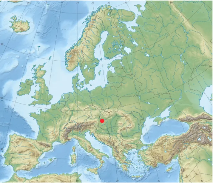
Figure 1: Present-day orography and bathymetry of Europe; from Wikipedia¹³². Shelves, which mostly fell dry during the LGM (Fig. 75), are colored in light blues. To reconstruct the mineral dust cycle for the LGM in Europe (Sec. 7.4), an analysis of the wind regime frequencies (Sec. 6) is required.

These Circulation Weather Type frequencies were calculated for a region labeled Transdanubia (Sec. 7.4, p. 98) that is centered around 47.5°N, 17.5°E (red dot). Transdanubia encompasses the Eastern Alps, the northern Dinarides, the Balkans, and the Carpathians (cf. also Fig. 18).

The Laurentide⁷²(LIS, up to ∼3600 m height), Greenland (GIS), and Eurasian ice sheet (EIS) cov- ered⁷²large parts of the Northern Hemisphere during the LGM. On northern Europe, the EIS mar- gin was several hundred meters thick, and the EIS thickness increased up to ∼2400 m at its center⁷². The EIS encompassed the Scandinavian ice sheet (SIS, also called Fennoscandian ice sheet), the British-Irish (BIIS), the Svalbard, the Barents Sea, and Kara Sea ice sheet. It covered¹¹Europe from the Arctic (∼80°N) to ∼50°N, thereby increasing the northern European topography distinctly¹³³. Moreover, the southeast sector of the SIS and the Alpine ice sheet reached their maximum about coterminously to the global LGM¹³⁴.

The LGM lake levels differed¹³⁵from today. An Italian lake and a lake in southern France were drier, whereas two lakes, one at the Balkans and one in southern Turkey, were much wetter¹³⁵.

2.3 Temperature distribution

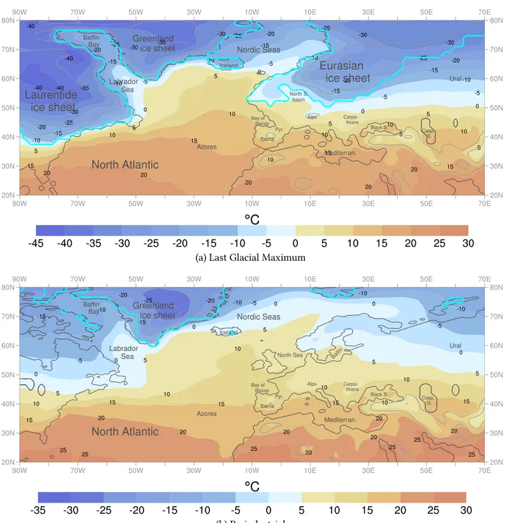
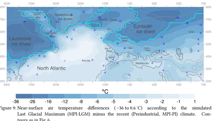
Compared with today, the LGM atmosphere was colder and drier^136–140. The mean global LGM near-surface air temperature differed49,129,141,142 by Δ𝑇 = −4.5±0.5^∘C from its present value. Compared to today, during the average European LGM winter, the simulated 2 m air temperature decreased⁶⁴ between 8 and 16^∘C in agreement with a pollen-reconstructed annual mean temperature decrease¹¹⁶ of Δ𝑇 = −12±3^∘C in western Europe. There, the coldest month cooled¹¹⁶ by Δ𝑇 = −30±10^∘C and the precipitation north of the Mediterranean decreased¹¹⁶ byΔ𝑃 = −800±100 mm, i.e.−60±20%, compared to today. Over the ice-sheet free central European regions, the annual average temperatures decreased between −5 and −10^∘C according to a regional simulation¹¹¹. According to paleobotany¹¹⁶, the cooling and drying at the LGM was more pronounced in western than in southeastern Europe. This gradient of decreasing temperatures was in line with more severe western than eastern European cooling, which was reported¹⁴⁰ as necessary for reproducing the LGM glaciers. Coherently, the polar front⁶⁶ and the westerlies⁷³ were shifted southward causing a drier climate116,140,143. For regions south of the Pyrenees–Alps line, temperature decreased by Δ𝑇 = −10±5^∘C according to pollen records¹¹⁶. For central Poland between 26 and 24 kyr ago, the mean annual temperature was −4^∘C, the intra annual temperature ranged between−27and 8^∘C, both reconstructed from coleoptera⁷¹. Nearby the EIS margin at the NW Russian plains, ice wedges¹³⁶ indicated an average annual temperature below−6^∘C. The average simulated LGM summer temperature decreased⁶⁴ by at least -16 to -8^∘C over the Scandinavian ice sheet compared to modern day summer temperatures in Scandinavia.

The Eurasian Arctic climate between 20 and 15 kyr ago was extremely cold and dry¹³⁶. Simi- larly, during the LGM, the northeastern Mediterranean was very cold and extremely dry⁸⁰; pollen evidence even for the whole Mediterranean strong dryness¹¹⁶. Also, the Carpathian Basin was drier⁵¹.

2.4 Greenhouse gas concentrations during the LGM and until today

Greenhouse gas concentrations were considerably lower during the LGM^78,144than at present time.

For the present (2018), CO₂concentration observations result in more than 400 ppmv. This value is strictly increasing at increasingly high rates on the multi annual scale since the onset of direct measurements¹⁴⁵.

The most prominent continuous direct measurement of the CO₂concentration is represented by the Mauna Loa Observatory (Hawaii, United States) time series¹⁴⁵that was started by David Keel- ing in March 1958. Laboratory analyzes of the Vostok ice core (Fig. 2) resulted⁷⁸in a mean CO₂con- centration of ∼185 ppmv (CH₄: ∼360 ppbv) for the LGM, i.e. until today, the CO₂concentration has more than doubled compared to the LGM.

Figure 2: LGM to Holocene CO₂(circles), CH₄(diamonds), and deuterium (δ D, solid curve, not discussed) concentrations based on the Vostok Dome C ice core measurements. The depth (top axis) is only valid for the CO₂ and CH₄ records. Younger Dryas (YD), Bølling/Allerød warm phase (B/A).

From Monnin et al.⁷⁸© AAAS (p. 195).

From the LGM to the present, the CO₂ concentration has increased by more than 215 ppmv (CH₄ by more than 1485 ppbv). Based on numerous evidence, such as the Vostok ice core⁷⁸ and the Mauna Loa measurements¹⁴⁵, this increase occurred at considerably varying rates including short periods of CO₂decrease during the last 18 kyr.

Between 17 and 10 kyr ago, the CO₂concentration increased monotonically⁷⁸by 75 ppmv reach- ing ∼268 ppmv¹⁴⁶. For the industrialization onset (1760), Antarctic climate archive CO₂concentra- tion reconstructions^147,148 resulted in ∼278 ppmv. This implies a total, yet not necessarily mono- tonic, increase of about 15 ppmv over ∼10 kyr. This increase is explainable by forest clearance through humans, first evidenced¹⁴⁶ for China (9400 years ago), then India (8500 years ago), then southern-central Europe (between 8000 and 7000 years ago).

At about 5000 years ago, the methane (CH₄) concentration started rising, as the Antarctic cli- mate proxies show¹⁴⁶. Synchronously, humans started irrigating rice¹⁴⁶and it is well known, that farming and irrigating rice releases methane¹⁴⁹. The methane concentration increase found in ice cores for the subsequent millennia can be explained as a direct consequence of ongoing rice irrigation and farming¹⁴⁶. This methane release amplified the greenhouse effect. Though the life- time of methane is shorter, its greenhouse effect per molecule is far larger^22,23,150 than that of CO₂. As the exponential human population density increase occurred first in southeastern Asia, it is also most likely that the extensive anthropological land use changes, which considerably trans- formed the previously ecosystems (shaped by hunters and gathers), also remain traceable in the cryospheric CH₄and CO₂concentration archives.

From 1760 to 1958, during about 200 years only, the CO₂concentration rose by ∼40 ppmv, from

∼278 to 316 ppmv^147,148. This strong acceleration of CO₂increase is directly related to the human- induced industrialization starting in Britain, then expanding over western Europe and subsequently over most mid-latitude regions of high population densities around the globe. From 1958 to the present¹⁴⁵, the CO₂ increase accelerated dramatically: The CO₂ concentration rose by another 84 ppmv within only 60 years, according to all direct measurements¹⁴⁵(Fig. 3).

Such a high rate is unprecedented during the existence of Homo sapienson this planet. The se- vere impacts of this global, human-induced greenhouse gas release exposes the essential planetary resources at high risks of destruction. In the past, humans could rely on and benefit from an enor- mous amount of ‘services’ provided by the ecosystems of the Earth ‘for free’. These included the availability of potable water, fertile soils for farming, and sophisticated element cycles taking care of the human waste including the repair of local, human-induced ecosystem damages.

However, the accelerated human-induced greenhouse gas increase implies the human decision to expose their current existence at risk in the upcoming years to centuries by increasing the like- lihood for systematic destruction. The acidification of the oceans, which take up one quarter of the released anthropogenic CO₂, leads to the collapse of key organisms^151–156 such as corals, crabs, oysters, and some plankton (calcifiers) — just to mention one of many current ecosystem threats.

Figure 3: Atmospheric CO₂concentration, observed since 1957. From Betts et al.¹⁴⁵. Extrapolated CO₂con- centration has been removed. © Macmillan Publ. Ltd (p. 195)

2.5 Biosphere

Generally, a lower CO₂ concentration, such as during the LGM, favors the photosynthesis of C₄ vs. C₃ plants^157,158. Yet, to determine the actual change of specific biomes, the precipitation and temperature that affects them must also be factored in^158,159. If photosynthesis is not limited by water stress nor by temperature, then the C₄outperform the C₃plants if both are subjected to a lower CO₂concentration^158–161. According to the Chinese Loess Plateau records, the temperature has to be higher than 15^∘C for the existence of C₄ plants in an originally C₃-dominated plant biome under lower CO₂ concentration¹⁶². Also, the precipitation increase needed by grasses is less than by trees under reduced CO₂conditions¹⁶¹. As a result, open vegetation such as steppe, tundra, or grassland, replaced forests^67,163; in particular grasses expanded their ecological range during the LGM¹⁶¹. For example, C₃grassland was favored instead of shrubs in eastern Europe, according to modeling results¹⁶¹ for the LGM. Besides grassland, central and eastern Europe was partly covered by taiga or montane woodland containing isolated pockets of temperate trees during the last full glacial¹⁶⁴. Simulations¹⁶⁵ and pollen¹⁶⁶ confirm more extensive herbaceous- and reduced shrub-tundra, which favored erosion and detrital sedimentation^80,167, in particular on grassland.

In Spain, southern France, Italy, Greece, Turkey, and southern Ukraine, cool¹¹⁶steppe prevailed, according to pollen^70,168. Consistently, in Italy, the Carpathian Basin, Dinarides, Balkans, northern France, the Benelux, the percentage of trees was below 20% during the LGM, while it could have been up to 40% in Spain and southern France, according to a principle component analysis¹⁶⁶ of pollen. At Monticchio in southern Italy, steppe prevailed¹¹⁷, according to a Mediterranean sed- iment core and lake sediments. Tropical semi-desert existed¹⁶⁷ in Turkey and Lebanon during the LGM. Northern France, the Benelux and unglaciated regions of Denmark, Germany, western Poland, and the United Kingdom were partially polar deserts¹⁶⁷.

On the Russian Plain, subarctic tundra (nearby the EIS) and steppe (nearby the Black Sea) dom- inated — whereas forest occurred fragmentarily¹⁶⁹. Particularly the northwestern Russian Plain was shaped by very dry climate³⁶and (sub-)Arctic vegetation¹³⁶. In the zone from western Ukraine to western Siberia, steppe graded into tundra¹¹⁵.

Taiga prevailed at the north coast of the Sea of Azov during the LGM¹¹⁵. Thus, it expanded about 1500 km southwards of its current limit in west Russia. Broadleaved trees were confined to small refuges¹¹⁵, such as the east coast of the Black Sea (cool mixed forest) and western Georgia (cool conifer forests). Their interglacial Caucasian-Georgian habitat was offset during the LGM by more than –1000 m in height¹¹⁵.

During the LGM, the Danube-region was relatively warmer than other European regions¹⁷⁰. The grass-covered east Carpathians were characterized by burning biomass, according to loess-charcoal analyzes¹⁷¹. These are in contrast to the globally decreasing trend of fires during the LGM¹⁷¹. However, they coincide with humans present in that region at the LGM¹⁷¹. The Carpathian Basin (CB) was much drier, particularly in its south, according to palaeopedology and loess⁹¹ (Surduk, 45.1°N, 20.3°E). On the river flood plains in the CB, wet or mesic grassland dominated, whereas outside of them, dry steppe prevailed¹⁷¹. Woods occurred in the river valleys and on wet, north-facing hillsides of the CB¹⁷¹. Scattered trees were likely present on the CB loess plateaus¹⁷¹. Consistently, grassland and taiga was reported⁵⁷ for the CB between 28 and 12 kyr ago.