International Real Business Cycles in the Developed and Emerging Economies of NAFTA and the EU
Inauguraldissertation zur
Erlangung des Doktorgrades der
Wirtschafts- und Sozialwissenschaftlichen Fakultät der
Universität zu Köln
2008
vorgelegt von
Esther Elisabeth Conrad, M.A.
aus Bielefeld
Erstgutachter: Professor Dr. Axel A. Weber Zweitgutachter: Professor Dr. Peter Funk Tag der Promotion: 03. Juli 2009
Erklärung
Ich erkläre hiermit, dass ich die vorgelegte Arbeit ohne Hilfe Dritter und ohne Benutzung anderer als der angegebenen Hilfsmittel angefertigt habe. Die aus anderen Quellen direkt oder indirekt übernommenen Aussagen, Daten und Konzepte sind unter Angabe der Quelle gekennzeichnet. Bei der Auswahl und Auswertung folgenden Materials haben mir die nachstehend aufgeführten Personen in der jeweils beschrieben Weise unentgeltlich geholfen:
Die Humboldt Universität in Berlin, die mir Zugang zu den in Kapitel 2 verwendeten Datensätzen ermöglichte.
Weitere Personen waren an der inhaltlich-materiellen Erstellung der vorliegenden Arbeit nicht beteiligt. Insbesondere habe ich hierfür nicht die entgeltliche Hilfe von Vermittlungs- bzw.
Beratungsdiensten in Anspruch genommen. Niemand hat von mir unmittelbar oder mittelbar geldwerte Leistungen für Arbeiten erhalten, die im Zusammenhang mit dem Inhalt der vorgelegten Dissertation stehen. Die Arbeit wurde bisher weder im In- noch im Ausland in gleicher oder ähnlicher Form einer anderen Prüfungsbehörde vorgelegt. Ich versichere, dass ich nach bestem Wissen die reine Wahrheit gesagt und nichts verschwiegen habe.
Berlin, 02. Mai. 2008
Esther Conrad
To my parents, to Eva and Charlotte
and to my dog, Loki
In addition I want to thank the following persons and institutions: My mother for her infinite patience and support, my advisor Professor Dr. Axel A. Weber for his patience and willingness to see this project through to the end, Prof. Dr. Andreas Schabert for pointing me in the right direction, Helge Budde and Sabine Liebe for always being there, Sylvia Weber and Bernhard Kerp for helping me manage time, Frank Bielig for showing me another way, and the Humboldt University in Berlin for giving me access to key data.
Berlin, 02. Mai. 2008
Esther Conrad
Abstract
This study empirically and theoretically evaluates economic interdependence of emerging and developed economies in terms of business cycles. In addition to evaluating Mexico’s business cycles relative to the developed NAFTA economies, it considers the business cycles of some of the Eastern European emerging economies in the EU relative to developed EU economies.
By evaluating intra- and cross-country statistics, the study finds that are empirical regularities (stylized facts) for emerging economies just as there are for developed ones. A key empirical finding is that developed economies belonging to the same trade agreement tend to have highly synchronized business cycles and hence positive output and consumption correlations, but that this relationship does not necessarily hold with respect to emerging economies. In fact, the correlations are virtually absent and sometimes even negative when comparing the emerging economies’ business cycles with those of their developed trading partners. It is shown that the intra-country statistics for both types of economies can successfully be reproduced using a one-country international real business cycle model with an endogenous interest rate. In addition, the non-existent or negative output and consumption correlations between the two economy types can be captured by a two-country international real business cycle model using portfolio adjustment costs and applying negative spillover effects in the productivity process of the emerging economy. The negative spillover effect also allows for a reversal of the usual theoretical implication of theses model types that there should be more consumption- than output smoothing (while data shows the opposite to be true). The study additionally gives a comprehensive overview of contemporary solution mechanisms used to solve this class of models.
I
I n d e x
Index ... I List of Tables ... IV List of Figures ... VI
Chapter 1: Introduction ... 1
1.1 Literature and Summary for Chapter 2 ... 3
1.2 Literature and Summary for Chapter 3 ... 5
1.3 Literature and Summary for Chapter 4 ... 7
Chapter 2: Measuring Business Cycles in Developed and Emerging Economies ... 9
2.1 Empirical Results ... 11
2.1.1 Intra-Country Findings ... 13
2.1.2 Cross-Country Findings ... 21
2.2 Concluding Remarks Chapter 2 ... 35
Chapter 3: Modeling Real Business Cycles of Developed and Emerging Economies ... 37
3.1 The Debt Elastic Interest Rate Model ... 39
3.2 The Steady State ... 45
3.3 Model 1: Calibration and Results for a Developed Economy ... 48
3.3.1 Impulse Response Analysis for Model 1 ... 51
3.3.2 Empirical vs. Theoretical Business Cycle Moments for Model 1 ... 55
3.4 Model 2: Calibration and Results for an Emerging Economy ... 58
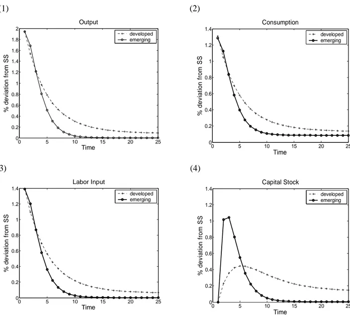
3.4.1 Impulse Response Analysis for Model 2 ... 62
II
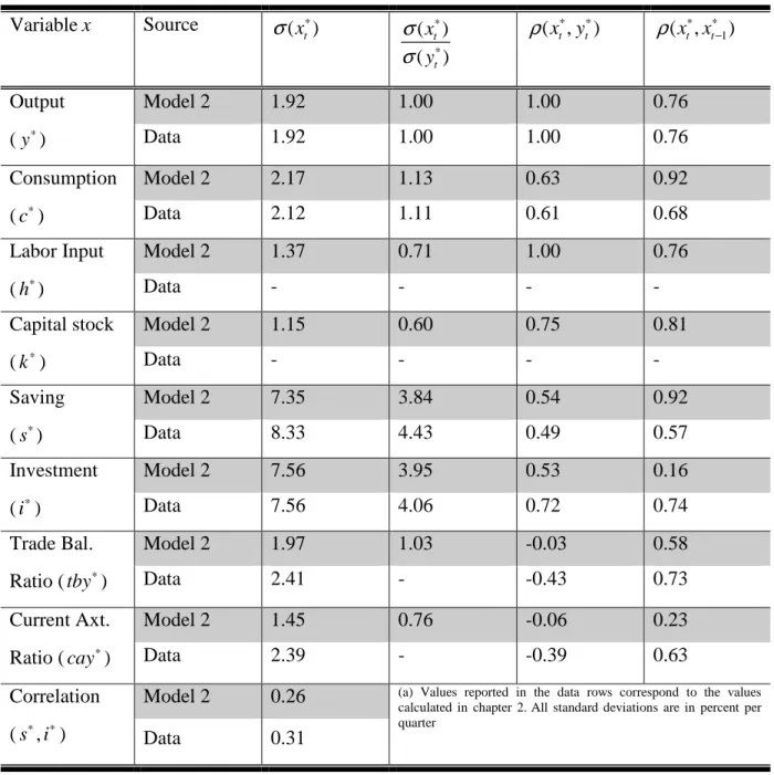
3.4.2 Empirical vs. Theoretical Business Cycle Moments for Model 2 ... 65
3.5 Model 3: Calibration and Results for a Two-Country Model of a Developed and Emerging Economy ... 67
3.5.1 Impulse Response Analysis for Model 3 ... 75
3.5.2 Empirical vs. Theoretical Business Cycle Moments for Model 3 ... 83
3.6 Concluding Remarks Chapter 3 ... 85
Chapter 4: A Primer on Solving Open Economy SDGE Models ... 87
4.1 Log-Linearizing the Debt Elastic Interest Rate Model ... 91
4.2 Derivation of Model 4 ... 94
4.2.1 Solution Stability and Uniqueness of Model 4 ... 97
4.2.2 Characterizing the Solution of Model 4 ... 100
4.3 The Method of Undetermined Coefficients ... 102
4.3.1 Interpreting the Undetermined Coefficients ... 106
4.4 The Eigenvalue Decomposition ... 109
4.4.1 Applying the Eigenvalue Decomposition to Model 4 ... 109
4.5 The Schur (QZ)-Decomposition for Higher Dimensional Models ... 113
Chapter 5: Conclusion ... 122
Chapter 6: Appendices ... 126
6.1 Data Appendix A: Chapter 2 ... 126
6.2 Technical Appendix B: Chapter 3 ... 128
6.2.1 Solving the Optimization Problem ... 128
6.2.2 Differentiation Needed for Steady State Determination ... 129
6.2.3 A Theoretical Discussion of Impulse Response Functions ... 131
6.2.4 Model 3: Remaining Business Cycle Statistics ... 133
6.3 Technical Appendix C: Chapter 4 ... 134
6.3.1 Linearizing the Trade Balance and Current Account ... 134
Ratios ... 134
6.3.2 The Eigenvalue Decomposition in the n-Variable Case ... 135
III 6.3.3 The Eigenvalue Decomposition: On the Role of the Stable Eigenvalue in
Transition Functions in Model 4 ... 144
6.3.4 The Schur-Decomposition: Reducing the Coefficient Matrix W ... 145
6.4 Computer Algorithms ... 147
6.4.1 Uhlig’s Toolbox ... 149
6.4.2 Oviedo’s Toolbox ... 151
References ... 154
IV
L i s t o f T a b l e s
Chapter 2
Table 2.1: Standard Deviations ... 14
Table 2.2: Selected Relative Standard Deviations ... 15
Table 2.3: Contemporaneous Correlation with Output ... 17
Table 2.4: Absolute and Relative Saving and Investment Correlations ... 19
Table 2.5: First-Order Autocorrelations ... 20
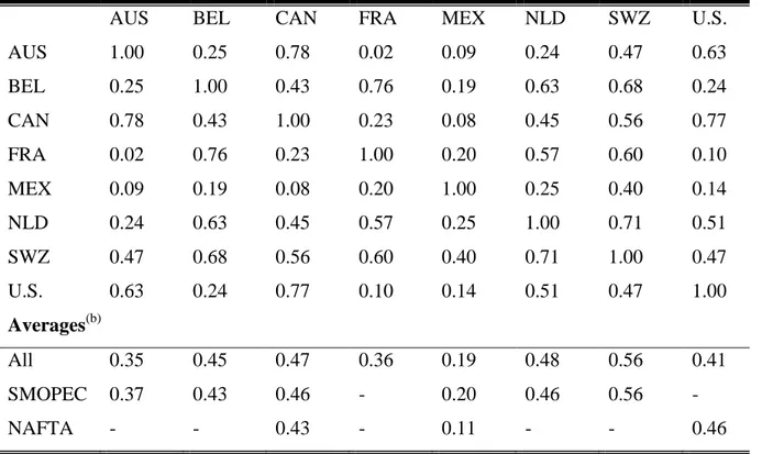
Table 2.6: Cross-Country Output Correlations ... 33
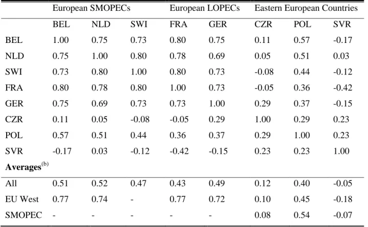
Table 2.7: Cross Country Output Correlations of European Countries Only ... 34
Table 2.8: Cross-Country Consumption Correlations ... 34
Table 2.9: Cross Country Consumption Correlations of European Countries Only ... 35
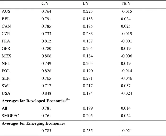
Chapter 3 Table 3.1: Averages of the Great Ratios ... 47
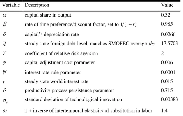
Table 3.2: Parameter Values for Model 1 (Developed Economy) ... 50
Table 3.3: Business Cycle Summary Stats: Model 1 vs. Average of Developed SMOPECs .. 56
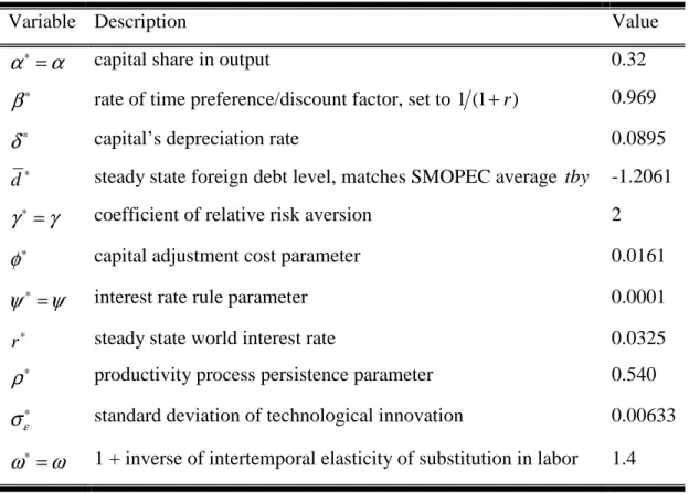
Table 3.4: Parameter Values for Model 2 (Emerging Economy) ... 61
Table 3.5:Business Cycle Summary Stats: Model 2 vs. Average of Emerging Economies .... 65
Table 3.6: Parameter Values for Model 3 (the Two-Country Model) ... 74
Table 3.7: Cross Country Business Cycle Summary Statistics : Model 3 vs. Data ... 84
Table 3.8: Intra-Country Business Cycle Summary Statistics: Model 3 vs. Data ... 84
V Chapter 4
Table 4.1: Variable Classification and Notation ... 90 Table 4.2: Policy and Transition Function Coefficients for Productivity in Model 4 (in %) 109
Chapter 6
Table 6.1: Additional Business Cycle Statistics of Model 3 ... 133 Table 6.2: Decomposing Uhlig’s Toolbox ... 151 Table 6.3: Decomposing Oviedo’s Toolbox ... 153
VI
L i s t o f F i g u r e s
Chapter 2
Figure 2.1: Synchronized Canadian and U.S. Business Cycles ... 23
Figure 2.2: Business Cycles in Countries Belonging to a Common Trade Agreement ... 24
Figure 2.3: The Eastern European Countries’ Output Cycle vs. the EU LOPECs... 26
Figure 2.4: The Eastern European Countries’ Output Cycle vs. the EU SMOPECs ... 28
Figure 2.5: The Eastern European Countries’ Consumption Cycle vs. the EU LOPECs ... 29
Figure 2.6: The Eastern European Countries’ Consumption Cycle vs. the EU SMOPECs ... 31
Chapter 3 Figure 3.1: Impulse Response Functions of the Developed Economy (Model 1) ... 52
Figure 3.2: Impulse Response Functions of the Emerging Economy (Model 2) ... 62
Figure 3.3: Impulse Response Functions of Model 3 after a One Percent Increase in the Technological Innovation of the Developed Economy Only ... 77
Figure 3.4: Impulse Response Functions of Model 3 after a One Percent Increase in the Technological Innovation of the Emerging Economy Only ... 80
Figure 3.5: Impulse Response Functions of Model 3 after a One Percent Increase in the Technological Innovation of Both Economies ... 81
Chapter 4 Figure 4.1: The Characteristic Polynomial of the Matrix A for Model 4 ... 99
1
C h a p t e r 1
Introduction
As globalization pushes countries into ever increasing, supranational interdependence, the nature of economic ties between developed and emerging economies is catapulted to the forefront of public debates. The word interdependence hosts ‘dependence’, a word that in light of the recent housing, banking, oil and food shortage crises that have propagated through developed and emerging economies alike, gains even more of a negative connotation.
Conversely, the ability of some economies to realize unprecedented growth through globalization, specifically via trade and more specifically via their ability to exploit their comparative advantages (think China), elicits more positive emotions. In short, economic interdependence is a topic inquisitive minds should grapple with.
Three issues (that certainly do not exhaust the potential spectrum of issues) come to mind: The first is a simple matter of measurement: How interdependent are economies of similar or different development types, how has this changed over time and how do regional aspects factor into interdependence? The second issue is how real business cycle analysis, which has proven vastly successful in modelling the business cycles of developed economies, can help us understand the behaviour of emerging economies and the interaction between emerging and developed economies. The last issue is qualitative: Do the benefits of interdependence outweigh the potential pitfalls? In other words, is the interdependence of business cycles dangerous (can one country’s recession drag down another leading to a
“domino effect”?) or does it lead to greater prosperity for all involved?
This study is mainly concerned with addressing the first two issues from a quantitative perspective and only treats the qualitative debate on the desirability of interdependence on the periphery. The five main findings are:
(1) There are empirical regularities for emerging economies similar to the ‘stylized facts’
that have been found for developed economies in the real business cycle literature.
2 (2) Two and half decades of data show that developed economies within close geographical proximity to one another or belonging to the same trade agreement tend to have highly synchronized business cycles, while the emerging economies’ business cycles with respect to their developed neighbors or trading partners display little synchronization.
(3) Many empirical features of both the developed as well as the emerging economies can successfully be reproduced with an international real business cycle model based on an endogenous interest rate.
(4) It is also theoretically possible to capture the lack of business cycle synchronization across the two economy types in a two-country model using portfolio adjustment costs and negative spillover effects in the productivity process of the emerging economy.1 (5) Even though the desirability of linked business cycles has lost some of its shine due to
the recent events mentioned above, it remains a fact that countries with highly synchronized business cycles are the more prosperous ones and that such a harmonization is therefore likely to be more advantageous than not.
The following chapters first establish intra-country and cross-country business cycle statistics for developed and emerging economies in North America and Europe. The countries were chosen depending on the reliability and availability of data and because the issues surrounding economic interdependence have been particularly poignant for them in recent years as they entered comprehensive trade agreements. Second, the question as to what kind of international real business cycle model can be used to reproduce the empirical intra- and cross-country data findings for both types of economies is taken up. These topics are treated in chapters 2 and 3 respectively. Chapter 4 gives an in-depth treatment of contemporary solution mechanisms for stochastic dynamic equilibrium (SDGE) models, with an application to one of the models introduced in chapter 3. Chapter 5 offers concluding remarks, while chapter 6 provides data and technical appendices to chapters 2 – 4. The remainder of chapter 1’s introduction provides a brief overview of the related literature for each chapter followed by a chapter summary.
1 This theoretical mechanism translates into allowing emerging economies to exploit their comparative advantage.
3
1.1 Literature and Summary for Chapter 2 (Measuring Business Cycles in Developed and Emerging Economies)
Studies on business cycles in developed economies are abundant, while analyses of business cycles in emerging economies are, as of yet, more of an ‘up-and-coming’ research trend. After being dormant for several decades, modern real business cycle (RBC) research was reignited by the work of Kydland and Prescott (1982). Initially most RBC studies focused on the United States (U.S.) using closed economy models. Starting in the early nineties, however, the models received more of an international flair: Mendoza (1991) estimated a small open economy model for Canada. Baxter and Crucini (1993) delivered a comprehensive overview of international business cycle frequencies for a selection of small and large economies and developed a model that could account for the saving-investment correlation puzzle (which finds a home-bias in saving). Backus, et al. (1992) were among the first to discover that a two-country real business cycle model (calibrated for the United States versus a European aggregate) generates higher consumption than output correlations – a finding that is at odds with the data. Stockmann and Tesar (1990) and Zimmermann (1995) are additional useful references on business cycle statistics for developed economies. More recent studies focus on emerging economies as well: Uribe and Yue (2006), for example, study interest rate premia for a set of emerging economies using a real business cycle model with habits, a working- capital constraint and debt adjustment costs. García-Cicco, et al. (2006) develop a real business cycle model with growth, an endogenous interest rate and a combination of transitory and permanent shocks, which they then compare to Argentine data. They find that the model is not able to account for Argentine business cycles. Neumeyer and Perri (2005) present a range of business cycle statistics for emerging economies and then develop a model with working-capital and an endogenous interest rate subject to interest rate shocks. Also calibrated to Argentina, they find (contrary to García-Cicco, et al. (2006)) that their model can generate results that are coherent with the data. Aguiar and Gopinath (2007) examine an even broader country set and create a model that successfully mimics the behavior of both a developed (Canada) and an emerging economy (Mexico). In addition they provide a precise decomposition of transitory and permanent shock components to productivity.
4 The emerging and developed economies of chapter 2 were chosen based on their geographical proximity to one another and their membership in a common preferential trade agreement (with two exceptions noted below). The first group is given by the countries belonging to the North American Free Trade Agreement (NAFTA): The developed ones are Canada and the U.S., the emerging one is Mexico. The second group is given by European countries, which, with one exception, belong to the European Union (EU): Here the developed countries are given by Belgium, France, Germany, the Netherlands and Switzerland (not an EU member), while the emerging ones are given by the Czech Republic, Poland and the Slovak Republic. Australia is included additionally as a ‘wild card’.
Chapter 2, in line with other research, confirms several empirical regularities (stylized facts) regarding the business cycles of the developed economies considered in this study:
Most prominently, consumption tends to be less volatile than output, labor input is about as volatile as output, capital is about half as volatile as output and investment is about three times more volatile than output (all measured by standard deviations), while net exports and the current account tend to be acyclical. In addition, cross-country comparisons of the developed economies generate positive consumption and output correlations, although there appears to be more output than consumption smoothing (a puzzling and robust feature of the data, which Backus, et al. (1992) were among the first to discover). For the emerging economies of chapter 2, the variables are generally more volatile than in developed economies, although the ranking of the variables’ volatility remains approximately the same.
The main exceptions are that the relative consumption to output volatility is larger than one (versus less than one in developed economies) and that the international variables tend to be much more countercyclical.
Chapter 2 also provides some insight on a topic that seems to have received little attention in the literature so far: The cross-country correlations for countries in the same vicinity but of a different development level. Even though consumption and output correlations across the developed economies in both the North American and European group indeed tend to be positive, the same correlations tend to be non-existent or even negative when comparing a developed and an emerging economy. Paradoxically, this is sometimes even more pronounced for neighboring countries belonging to the same regional preferential trade agreement – a fact that initially seems counterintuitive. Theoretically one ought to expect that positive productivity shocks translate into greater spillover effects (and hence positive output and consumption correlations) for countries with little geographical distance between them or for countries sharing membership in a regional trade agreement or both.
5 Although the business cycles of the developed economies in each of the two geographical groups exhibit precisely this behavior, emerging economies vis-à-vis their developed neighbors and preferential trade partners do not. As mentioned, the answer to this puzzle may be that spillover effects do not disseminate equally in both directions. Rather a positive spillover of productivity shocks going from developed to emerging economies but a negative spillover effect going from emerging to developed economies may be the source of the discrepancy. A negative spillover effect, as explained in chapter 3, could be interpreted as a mechanism that allows the emerging economy to exploit its comparative advantage at the expense of the developed economy. With negative spillover effects, a positive productivity shock in the emerging country would, ceteris paribus, eventually lead to a decline in the productivity of the developed country and could therefore explain the lack of business cycle synchronization
1.2 Literature and Summary for Chapter 3 (Modeling Real Business Cycles of Developed and Emerging Economies)
Some of the literature related to chapter 2 relates to chapter 3 as well. Modifications to the standard, non-stationary open economy model are presented by Mendoza (1991), Schmitt–
Grohé and Uribe (2001, 2003) and Kim and Kose (2003), who all examine the role of an endogenous discount factor2 as a stationarity–inducing mechanism in an open economy SDGE model. Schmitt–Grohé and Uribe (2003) give a comprehensive overview on small open economy real business cycle models by comparing and contrasting five modeling specifications: (1) a model based on an endogenous discount factor which either depends on the average per capita level of consumption or on a representative agent’s consumption level, (2) a model featuring a debt elastic interest rate premium, (3) a model including portfolio adjustment costs to debt holdings, (4) a complete asset market model and (5) the standard non-stationary open economy model. They conclude that each of the stationarity–inducing
2 Also known as Uzawa type preferences, where individuals become more impatient the more they consume. See Uzawa (1968)
6 instruments just mentioned predict similar dynamics and that the computationally more involved endogenous discount factor model is therefore the least parsimonious –if the researcher’s aim is to simplify numerical approximations. Kim, et al. (2001) compare the welfare implications of complete versus incomplete asset markets in the context of an endowment economy. Two country models have been examined by Kollmann (1996, 1998) using an incomplete asset market structure while Backus, et al. (1992) and Baxter and Crucini (1993) are among the standard works for two-country models with a complete asset market structure.
Chapter 3 is based on two of the small open economy models discussed in Schmitt–
Grohé and Uribe (2003): The first incorporates an interest rate premium (i.e. an endogenous interest rate) and the second uses portfolio adjustment costs, both of which are a function of deviations of debt from the steady state. The interest rate premium model is used twice, once to match selected data features for an average of the developed economies introduced in chapter 2 (model 1) and once to match the same features for an average of the emerging economies (model 2).3 The portfolio adjustment cost approach is used in a two-country model (model 3), which is primarily calibrated to match the characteristics of cross-country consumption and output correlations between averages of the emerging and developed economies. It turns out that an interest rate premium model (models 1 and 2) is not just able to capture statistical features of the developed economies but of the emerging economies as well (a contended issue in the literature). Additionally, using some potentially unconventional parameterization for the exogenous productivity process (i.e. by allowing for the possibility of negative spillover effects), the two-country portfolio adjustment cost model is able to match the virtually non-existent consumption and output correlations between the two types of economies and reverses the ‘usual’ modeling implication that there should be more consumption than output smoothing.
The use of either an endogenous interest rate premium or a portfolio adjustment cost function in a small open economy model is a way to ensure that the steady state is well defined and the solution stationary. A standard small open economy model without such mechanisms can exhibit infinite second moments because either steady state consumption or debt are not well defined. According to Schmitt-Grohé and Uribe (2003), this can imply that
“endogenous variables … wonder around an infinitely large region in response to bounded
3 An alternative to taking averages for each type of economy would be to choose one representative emerging and developed economy as in Aguiar and Gopinath (2007) who chose Mexico and Canada. The reason this was not the course of action chosen here is because the Eastern European countries and Mexico at times display very different results.
7 shocks. This introduces serious computational difficulties because all available techniques are valid locally around a given stationary path” (p.164). It should be intuitive that the interest rate premium and the portfolio adjustment costs increase in a country’s debt obligations (or decrease in a country’s assets holdings).
Both model types feature incomplete asset markets. The use of an incomplete rather than a complete asset market is necessitated by the statistical findings of chapter 2, which reveal a low and sometimes even negative consumption (as well as output) correlation among developed and emerging economies. It is a well known fact, that complete asset market models, in which agents have access to a state contingent array of financial instruments, allow idiosyncratic risks to be pooled. As a result, high positive consumption correlations are created in two-country models, which would obviously constitute an incorrect modeling specification for the task at hand. In an incomplete asset market agents have access to a single risk free asset, which prevents excessive consumption and output smoothing and thereby generates lower correlations.
1.3 Literature and Summary for Chapter 4 (A Primer on Solving Open Economy SDGE Models)
The theoretical solution mechanisms underlying the kinds of international real business cycle models just mentioned are rooted in the work of Blanchard and Kahn (1980) and more recently in papers by Klein (2000) and Sims (2002). These authors show how to exploit a linear representation of a stochastic model with (potentially multiple) leads and lags of variables. The linearized model paves the way for the derivation of impulse response functions and the determination of business cycle summary statistics, which tend to be the ultimate goal of most analyses on this topic. A standard references on how to linearize these types of models is given by the contribution of King, et al. (2002). Uhlig (1997) and Oviedo (2005) also explain the linearization process in greater detail and elaborate and build on the theoretical solution methods by introducing intelligible computer toolboxes to solve this class of models. These are briefly discussed in the technical appendix to chapter 4 (chapter 6).
8 Second-order approximations are analyzed by Schmitt–Grohé and Uribe (2004) and will not be explored here, especially because first-order approximations usually render very accurate results. Kim and Kim (1999) take on this latter issue by examining why standard, first-order linear approximation methods sometimes imply higher welfare levels for models with incomplete versus complete asset markets. They propose a bias-correction which generates results as accurately as a second-order approximation.
Chapter 4 elucidates the underlying solution mechanisms for the models in chapter 3 by providing a primer (introductory treatment) on solving linearized small open economy SDGE models with an application to the interest rate premium model of chapter 3. In addition, chapter 4 provides a comprehensive overview of the methodological tools and the links between them. As it turns out, some key features of the interest rate premium model (models 1 and 2) can be retained even if domestic investment and the capital stock are kept constant, i.e. are always at their steady state level. The forced constancy of these two variables represents the simplification (this constitutes model 4) relative to models 1 and 2 presented in chapter 3. In effect, this amounts to eliminating one state variable (capital) from the linearized model, which can greatly facilitate the analysis if a researcher is interested in solving this kind of model via ‘back of the envelope’ calculations.
Two ‘traditional’ solution mechanisms, the method of undetermined coefficients and the eigenvalue decomposition, will be explored in the context of the simplified model. In the case of more complex models with more than two state variables, such as models 1 - 3 introduced in chapter 3, these types of calculations become virtually impossible and the Schur-or QZ-decomposition (the current standard of real business cycle solution algorithms) is required. The discussion on the eigenvalue decomposition will be particularly useful for understanding this more complex algorithm, since it is a special case of the Schur- decomposition.
9
C h a p t e r 2
Measuring Business Cycles in Developed and Emerging Economies
Studies of business cycles in emerging and developing economies can approximately be grouped into four sets of stylized facts that form the pillars of this chapter’s empirical analysis and are a proxy by which the accuracy of any model can be measured. These stylized facts can, for example, be found in the work of Backus and Kehoe (1991), Baxter and Crucini (1993) and Mendoza (1991) for developed economies. Additionally, more recent works of Uribe and Yue (2006), García-Cicco, et al. (2006), Neumeyer and Perri (2005) and Aguiar and Gopinath (2007) also focus on business cycles in emerging economies.
For developed economies the stylized facts are given by:
consumption is pro-cyclical and tends to be less volatile than output,4 labor input is pro-cyclical and tends to be as volatile as output, capital is acyclical and about half as volatile as output,
saving and investment are strongly pro-cyclical and about two to three times as volatile as output,
net exports are countercyclical and less volatile for large than for small countries, all of the above variables have strong positive first-order autocorrelations,
the real interest rate tends to be acyclical and lags the business cycle.
For emerging economies the stylized facts are similar to those of developed economies, with the following additions and modifications:
on average, variables are more volatile,
4 A pro-cyclical variable exhibits a positive contemporaneous correlation with output. An acyclical variable exhibits almost no contemporaneous correlation with output in either direction. A counter-cyclical variable exhibits a negative contemporaneous correlation with output. The volatility measure is given by a variable’s percentage standard deviation.
10 consumption tends to be more volatile than output rather than less,
saving and investment are much more volatile relative to developed economies, net exports are strongly countercyclical,
the real interest rate is counter-cyclical and leads the business cycle.
In terms of cross-country correlations for developed economies (these will be extended to emerging economies below) the main stylized facts are:
output and consumption are positively correlated across countries,
cross-country output correlation tends to be higher than cross-country consumption correlations.
An additional and frequently cited stylized fact in both closed and open economy real business cycle literature is the high correlation between saving and investment, a ‘puzzle’ that was initially discovered by Feldstein and Horioka (1980), who demonstrated that domestic saving and investment rates for sixteen OECD countries from 1960–1974 were highly correlated. By regressing investment on saving rates, the coefficient on the latter was found to be near unity in the sample average. This was interpreted as empirical evidence against international capital mobility. If capital were indeed mobile, then we should find no correlation between saving and investment since, in theory, higher domestic saving should be invested where returns are highest and not necessarily remain in the domestic market. This anomaly, especially for developed, large open economies (LOPECs) such as the U.S., has remained a robust empirical finding across two and a half decades of research.
This chapter examines a set of countries, including both developed and emerging economies, which also display the stylized facts mentioned above. In addition, the data sheds some light on new evidence regarding the cross-country correlations between developed and emerging economies. The most prominent finding is that even though consumption and output correlations across developed economies tend to be positive, the same correlations tend to be surprisingly non-existent or negative when comparing a developed and an emerging economy.
This is somewhat surprising, because a positive productivity shock in a non-autarkic country (which describes most countries today) should theoretically ‘spill over’ into other countries, at least to some extent. Perfect historical examples are the industrial revolution that began in Britain and then spread to the U.S. and Europe or the more recent personal computing revolution that emanated from the U.S. into the farthest corners of the world. It should be intuitive that positive productivity shocks can be expected to have greater spillover effects and
11 hence positive output and consumption correlations for countries with little geographical distance between them or for countries sharing membership in a regional trade agreement.
The countries in this chapter’s sample meet these criteria, but nevertheless display stark differences in output and consumption correlations depending on development level.
Although the ability of emerging economies to quickly internalize positive productivity shocks stemming from other countries may be impeded by factors such as an untrained workforce or by a lack of infrastructure, the preponderance and intensity of the negative correlations still seems striking. An explanation for this phenomenon is given in chapter 3, which considers the possibility that there may be negative spillover effects for the developed economies when the emerging economies experience positive productivity shocks.
2.1 Empirical Results
The set of developed economies examined is given by some of the typical small open economies found in the literature –Australia (AUS), Belgium (BEL), Canada (CAN), the Netherlands (NEL) and Switzerland (SWI) – as well as some larger open economies: France (FRA), Germany (GER) and the U.S. These developed economies have been the focus of numerous real business cycle studies and therefore present limited opportunities for new results, except in the sense that the data is as recent as 2006. The set of emerging economies is given by the Czech Republic (CZR), Mexico (MEX), Poland (POL), and the Slovak Republic (SLR). Although Mexico, and more generally various South American and Asian countries, have been the subject of several real business cycle studies focusing on emerging markets (for example, Aguiar and Gopinath (2007), Neumeyer and Perri (2005), García-Cicco, et al.
(2006), Uribe and Yue (2006) and Kydland and Zarazaga (2002)), the set of Eastern European countries has not.5 Because of the proximity of two developed economies, Canada and the U.S., to an emerging economy, Mexico, it is a logical experiment to compare these North American countries with the developed and emerging economies of Europe. Moreover, the North American countries share membership in the North American Free Trade Agreement
5 Notably, the Slovak Republic is actually included in the Aguiar and Gopinath (2005) country set, but Poland and the Czech Republic are not.
12 (NAFTA, established 1994), while the European countries share membership in the European Union (EU, established in 1992). Even though the Eastern European countries in question did not fully join the EU until 2004, they had significant access to the EU market via preferential trade agreements prior to their own accession. In particular, the Czech Republic and Poland began formal accession negotiations in 1998, while the Slovak Republic did so in 2000 (Beichelt (2004)). Australia and Switzerland obviously neither belong to the EU or NAFTA and in the case of Australia, there is also no geographical closeness relative to the rest of the sample. These two countries therefore serve as crosschecks for the obtained results.
The following applies to all data presented: All volatility measures (standard deviations) are based on the longest available data span for each series within each country, measured on a quarterly basis (see data appendix for more information). All correlations are based on the longest common sample of any two series within one country (these are intra- country correlations such as a country’s saving-investment correlation) or on the longest common sample of a series across two countries (these are the cross-country correlations such as two countries’ consumption correlation). Each series x is measured in constant prices it (real terms), then divided by the working age population to obtain per capita terms and lastly transformed into logarithms. The exceptions are the trade-balance to output ratio, the current- account to output ratio and the real interest rate, which are all in percentage terms. All series are detrended using the Hodrick-Prescott filter, setting the smoothing parameter λ=1600.
The (per capita) series considered are: real GDP (y ), real consumption (t c ), t excluding government consumption (g ), labor input (t h ) given by hours worked per t employee in the total economy multiplied by total employment, the capital stock (k ) given t by the volume of the total economy’s capital stock, saving (s ) given by t yt− −ct gt,6 real investment (i ), the trade-balance to output ratio (t tby ) obtained by dividing the current value t of net exports by the value of current GDP, the current-account to output ratio (cay ) given by t the current account as a percentage of current GDP and lastly the real interest rate series (r ), t which was taken from Neumeyer and Perri (2005) for Australia, Canada, the Netherlands and Mexico. Because of the difficulty to obtain comparable labor input and capital stock series, these variables were omitted for the emerging economies. For the developed countries, two average measures are considered: The first (All) takes the mean for all countries, the second eliminates the three largest economies France, Germany and the U.S. (the large open
6 This follows the definition used by Baxter and Crucini (1993). They also discuss why true saving are difficult to measure and why this definition might be the most parsimonious.
13 economies abbreviated as LOPECs) from the sample, leaving the small open economies (SMOPECs).
2.1.1 Intra-Country Findings
Table (2.1) and table (2.2) display absolute and relative (to output) standard deviations of each variable, confirming the stylized facts. In terms of table (2.2), consumption is less volatile than output in developed economies, resulting in a relative standard deviation of 0.85 for the average of all developed economies.7 This trend is reversed for the emerging economies, where consumption tends to be more volatile than output, yielding an average relative standard deviation of 1.13. For the set of all developed economies, labor-input displays similar volatility as output (yielding an average relative standard deviation of 1.03), while the capital stock is only half as variable as output (with an average relative standard deviation of 0.48). Saving and investment are approximately three to four times as volatile as output in developed economies (3.67 and 3.21 respectively), and are about four to five times as volatile as output in emerging economies (4.43 and 4.06 respectively). Lastly, table (2.1) shows that, in terms of absolute standard deviations, the trade balance and current account ratios are more than twice as volatile in emerging than in developed economies (for the trade balance ratio this is 2.41 in emerging versus 0.78 in developed economies and for the current account this is 2.39 in emerging versus 0.98 in developed).
7 Unless there is a big discrepancy, the averages across all developed economies will be emphasized rather than always distinguishing between SMOPECs and LOPECs.
14 Table 2.1: Standard Deviations σ( )xt (a)
( )yt
σ σ( )ct σ( )ht σ( )kt σ( )st σ( )it σ(tbyt) σ(cayt) σ( )rt
AUS 1.43 0.96 1.66 0.35 5.93 5.51 0.98 1.03 0.50
BEL 0.99 0.97 0.79 0.54 3.61 4.11 0.73 1.12 -
CAN 1.57 1.23 1.45 0.88 5.21 4.25 0.97 1.08 0.45
CZR 1.50 1.62 - - 5.70 5.15 1.58 2.12 -
FRA 0.82 0.77 0.72 0.38(c) 3.19 2.74 0.61 0.58 -
GER 0.88 0.91 0.74(b) 0.91 3.18 2.89 0.68 0.70 -
MEX 2.42 2.98 - - 5.16 9.47 2.04 1.91 0.68
NEL 1.18 1.17 2.28(b) 0.33(c) 3.75 3.56 1.02 1.41 0.22
POL 2.21 1.55 - - 14.51 6.55 1.77 1.26 -
SLR 1.53 2.31 - - 7.96 9.06 4.27 4.28 -
SWI 1.25 0.74 0.80 0.29(c) 3.76 3.11 0.82 1.42 -
U.S. 1.31 1.02 1.40(b) 0.64 5.96 3.68 0.40 0.48 -
Averages for Developed Economies(d)
All 1.18 0.97 1.23 0.54 4.32 3.73 0.78 0.98 0.39
SMOPEC 1.28 1.02 1.40 0.48 4.45 4.11 0.90 1.21 0.39
Averages for Emerging Economies
1.92 2.12 - - 8.33 7.56 2.41 2.39 0.68
Notes: (a) All standard deviations are in percentage points per quarter and based on the maximum number of available observations. See the data appendix for additional information. (b) Total hours worked in the business sector rather than the total economy. (c) The capital stock of the business sector rather than the capital stock of the total economy. (d) Average “All” refers to the average across all developed economies,
‘SMOPEC’ is the average obtained by excluding France, Germany, and the U.S. (the large open economies = ‘LOPEC’), leaving the small open developed economies (SMOPECs).
15 Table 2.2: Selected Relative Standard Deviationsσ(x yt t)(a)
( ) ( )
t t
c y σ σ
( ) ( )
t t
h y σ σ
( ) ( )
t t
k y σ σ
( ) ( )
t t
s y σ σ
( ) ( )
t t
i y σ σ
AUS 0.67 1.16 0.24 4.15 3.85
BEL 0.98 0.80 0.55 3.65 4.15
CAN 0.78 0.92 0.56 3.32 2.71
CZR 1.08 - - 3.80 3.43
FRA 0.94 0.88 0.46(c) 3.89 3.34
GER 1.03 0.84(b) 1.03 3.61 3.28
MEX 1.23 - - 2.13 3.91
NEL 0.99 1.93(b) 0.27(c) 3.18 3.02
POL 0.70 - - 6.57 2.96
SLR 1.51 - - 5.20 5.92
SWI 0.59 0.64 0.23(c) 3.01 2.49
U.S. 0.78 1.07(b) 0.48 4.55 2.81
Averages for Developed Economies(d)
All 0.85 1.03 0.48 3.67 3.21
SMOPEC 0.80 1.09 0.37 3.46 3.24
Averages for Emerging Economies
1.13 - - 4.43 4.06
Notes: See table (2.1)
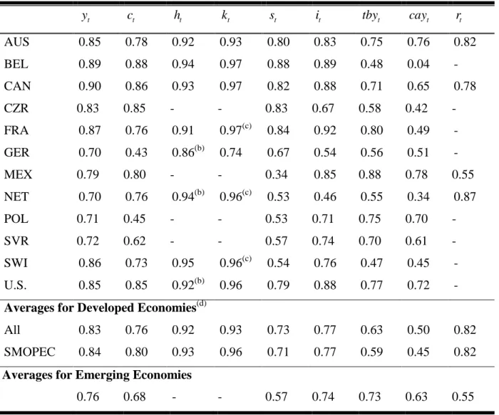
16 Table (2.3) shows that in all of the developed economies, consumption, labor input, saving and investment have positive contemporaneous correlations with output (0.71, 0.67, 0.81 and 0.79). These do not change much when considering the SMOPECs only. Capital is acyclical, yielding an average contemporaneous correlation with output of 0.17, while the correlation between the real interest rate and output for the three developed countries with available data can also be considered weakly pro-cyclical (0.51).8 In addition, both the trade balance and current account ratios are counter-cyclical (with correlation coefficients around - 0.30).
The contemporaneous output correlations in the emerging markets exhibit less similarities across the four countries. The consumption-output correlation, for instance, is much higher in Mexico (0.92) than in the Eastern European countries, where it is below 0.60 in all cases, which, with the exception of Australia (0.40), is also lower than for all the developed countries. Additionally, the saving-output correlation in the emerging economies is not as conform as in the case of the developed economies (ranging from 0.25 for the Slovak Republic to 0.71 for the Czech Republic). This variability may stem from the measurement difficulties associated with the saving definition (see second to last footnote). The investment- output correlation is not as variable as the saving-output correlation and, as is the case for developed economies, tends to be positive (0.72 for the emerging economies versus 0.79 for all developed economies). The trade-balance and current-account to output ratios are more counter-cyclical in emerging markets than in developed countries, with average correlation coefficients of around -0.40 (versus around -0.30 in the developed countries). Although the stylized fact that finds a stronger counter-cyclicality of the trade balance and current account ratios in emerging economies (relative to developed economies) is therefore confirmed, it is not as pronounced as in other studies (see for example, Aguiar and Gopinath (2007)). Lastly, although no generalization can be made due to the small sample on real interest rate series, it is confirmed that the interest rate is pro-cyclical in the three developed economies, while it is countercyclical (with a correlation coefficient of -0.47) for Mexico.
8 Neumeyer and Perri (2005) find an acyclical interest rate for their set of developed economies with an average output correlation coefficient of 0.20.
17 Table 2.3: Contemporaneous Correlation (ρ) of x with Output t yt(a)
(c yt, t)
ρ ρ(h yt, t) ρ(k yt, t) ρ(s yt, t) ρ(i yt, t) ρ(tby yt, t) ρ(cay yt, t) ρ(r yt, t)
AUS 0.40 0.66 -0.19 0.90 0.84 -0.43 -0.47 0.43
BEL 0.79 0.66 0.23 0.75 0.79 -0.51 -0.37 -
CAN 0.88 0.88 -0.07 0.93 0.74 -0.06 -0.18 0.50
CZR 0.59 - - 0.71 0.61 -0.43 -0.27 -
FRA 0.78 0.74 0.26(c) 0.84 0.87 -0.38 -0.26 -
GER 0.63 0.70(b) 0.23 0.72 0.76 -0.29 -0.39 -
MEX 0.92 - - 0.32 0.91 -0.62 -0.63 -0.47
NEL 0.70 0.56(b) 0.33(c) 0.83 0.71 -0.20 -0.27 0.59
POL 0.33 - - 0.68 0.67 -0.29 -0.33 -
SLR 0.58 - - 0.25 0.69 -0.39 -0.31 -
SWI 0.68 0.29 0.59(c) 0.65 0.70 -0.36 -0.12 -
U.S. 0.82 0.86(b) -0.01 0.86 0.94 -0.47 -0.49 -
Averages for Developed Economies(d)
All 0.71 0.67 0.17 0.81 0.79 -0.34 -0.32 0.51
SMOPEC 0.69 0.61 0.18 0.81 0.76 -0.31 -0.28 0.51
Averages for Emerging Economies
0.61 - - 0.49 0.72 -0.43 -0.39 -0.47
Notes: (a) All correlations are based on the maximum number of common observations. See the data appendix for additional information. (b) Total hours worked in the business sector rather than the total economy. (c) The capital stock of the business sector rather than the capital stock of the total economy. (d) “All” refers to the average across all developed economies, ‘SMOPEC’ refers to the average obtained by excluding France, Germany, and the U.S. (the large open economies = ‘LOPEC’), leaving the small open developed economies (SMOPECs).
18 Table (2.4) presents a stylized fact that is rooted in more recent research: Both in terms of absolute saving and investment and in terms of relative saving and investment rates (i.e.
ratios with respect to output), contemporaneous correlations between these two variables tend to be lower for emerging economies than for developed economies. Although a recent consensus has emerged that the Feldstein-Horioka puzzle has not been as pronounced in developed economies in recent years, it does manifest itself in individual cases (most notably the U.S. where the absolute (relative) saving-investment correlation equals 0.79 (0.65) or in Australia and Belgium, where the same correlations are 0.72 (0.53) and 0.73 (0.62) respectively). One reason that the saving-investment correlations have declined in recent years is likely to be due to greater capital mobility that emerged as a consequence of globalization beginning in the 1990s. In the emerging economies, however, the Feldstein- Horioka puzzle can hardly be said to exist. Here, the absolute (relative) saving-investment correlations range from -0.29 (-0.50) for the Slovak Republic to 0.56 (0.29) for Poland. When considering these values, the caveat regarding the potentially inaccurate measurement of saving should be kept in mind. On average, the absolute saving-investment correlation of 0.64 for all developed economies decreases to 0.54 once the LOPECs are omitted and decreases even further to 0.26 once only emerging markets are considered. For the relative saving- investment rate correlation, the average taken across all developed economies is 0.43, 0.40 for the SMOPECs alone, and -0.01 for the emerging economies. Thus, it is safe to conclude that in emerging economies absolute and relative saving and investment exhibit less contemporaneous saving and investment correlations relative to developed economies. The latter seem to exhibit increasingly less of the puzzling characteristics described by Feldstein and Horioka, even though the two variables are still positively correlated throughout the sample