Interactions between the real economy and the stock market

Interactions between the real economy and the stock market

Frank Westerhoff

Working Paper No. 84 December 2011

k*

b

0

B A M

AMBERG CONOMIC

ESEARCH ROUP

B E R G

Working Paper Series BERG

Bamberg Economic Research Group Bamberg University

Feldkirchenstraße 21 D-96052 Bamberg Telefax: (0951) 863 5547 Telephone: (0951) 863 2687 felix.stuebben@uni-bamberg.de

http://www.uni-bamberg.de/vwl/forschung/berg/

ISBN 978-3-931052-95-9

Redaktion:

Dr. Felix Stübben



felix.stuebben@uni-bamberg.de

1

Interactions between the real economy and the stock market

Frank Westerhoff

University of Bamberg, Department of Economics

Abstract

We develop a simple behavioral macro model to study interactions between the real economy and the stock market. The real economy is represented by a Keynesian goods market approach while the setup for the stock market includes heterogeneous speculators.

Using a mixture of analytical and numerical tools we find, for instance, that speculators may create endogenous boom-bust dynamics in the stock market which, by spilling over into the real economy, can cause lasting fluctuations in economic activity. However, fluctuations in economic activity may, by shaping the firms’ fundamental values, also have an impact on the dynamics of the stock market.

Keywords

Goods market, stock market, heterogeneous speculators, stability analysis, complex dynamics.

JEL classification D84, E12, G12.

____________

*

Presented at the International Conference on Rethinking Economic Policies in a Landscape of Heterogeneous Agents, Milan 2011, at the International Conference of the Society for Computational Economics on Computing in Economics and Finance, London, 2010, at the Workshop on Interacting Agents and Nonlinear Dynamics in Macroeconomics, Udine, 2010, and at the Workshop on Optimal Control, Dynamic Games and Nonlinear Dynamics, Amsterdam, 2010. Thanks to Carl Chiarella, Reiner Franke, Tony He, Cars Hommes, Blake LeBaron, Alfredo Medio and Valentyn Panchenko for their many useful comments and suggestions.

**

Contact: Frank Westerhoff, Department of Economics, University of Bamberg, Feldkirchenstrasse 21,

D-96045 Bamberg, Germany (email: frank.westerhoff@uni-bamberg.de).

2 1 Introduction

Over the last 20 years, many interesting agent-based financial market models have been proposed to study the dynamics of financial markets (for recent surveys, see Chiarella et al.

2009, Hommes and Wagener 2009, Lux 2009 and Westerhoff 2009). As revealed by these models, it is the trading activity of heterogeneous interacting speculators that accounts for a large part of the dynamics of financial markets. Even in the absence of stochastic shocks, intricate asset price dynamics may emerge in these models, for instance, due to the speculators’ use of nonlinear trading rules. Buffeted by stochastic shocks, however, these models are able to replicate some important statistical properties of financial markets remarkably well. Thanks to these models, phenomena such as bubbles and crashes, excess volatility and volatility clustering are now much better understood.

Overall, this line of research may be regarded as quite successful. Surprisingly, however, the attention of these models is typically restricted to the dynamics of financial markets. Put differently, the impact financial markets may have on other subsystems of the economy, such as the goods market, is widely neglected. And, of course, the impact other subsystems of the economy may have on financial markets is equally neglected. In this paper, we therefore develop a model in which a goods market is connected with a stock market, which we hope will improve our understanding of interactions between the real economy and the stock market. Given that there are a number of prominent historical examples

in which stock market crises have triggered severe macroeconomic problems – the Great Depression, the so-called Lost Decade in Japan and the recent Global Financial and Economic Crisis, to name just a few – this seems to us to be a worthwhile and important endeavor.

1

A deeper empirical investigation into this issue is provided by Kindleberger and Aliber (2005); however, see

also Galbraith (1997), Minsky (2008), Akerlof and Shiller (2008) or Reinhart and Rogoff (2009).

3

To be able to understand how our model functions, we keep it rather simple.

Moreover, we place greater emphasis on the model’s financial part than on its real part. One reason is that we can readily apply some basic insight from the field of agent-based financial market models here. Another reason is that the recent financial market turmoil has made it clear that financial market crashes may be quite harmful to the real economy. In a nutshell, the structure of our model is thus as follows. We represent the real economy with a simple Keynesian goods market model for a closed economy; our formulation of the stock market recognizes the trading activity of heterogeneous speculators. Ultimately, the goods market is linked to the stock market since both consumption and investment expenditures depend on the performance of the stock market. The stock market, in turn, is linked to the goods market since the stock market’s fundamental value depends on national income.

Obviously, there is a bi-directional feedback relation between national income and stock prices and, indeed, national income and stock prices are jointly driven by a two- dimensional nonlinear map. Based on analytical and numerical insights, we conclude that interactions between the real economy and the stock market may be harmful to the economy. Speculators may generate complex bull and bear stock market dynamics, leading to fluctuations in economic activity. In addition, fluctuations in economic activity affect the firms’ fundamental values and may amplify stock market dynamics. However, speculate activity may not always be welfare decreasing. Under some conditions, a permanent stock market boom may create a permanent economic boom.

The remainder of our paper is organized as follows. In Section 2, we introduce our

model and relate it to the literature. In Section 3, we present our analytical results, for both

isolated and interacting goods and stock markets. In Section 4, we extend our analysis using

numerical methods and explain what drives the dynamics of our model. In Section 5, we

conclude and point out some extensions for future work.

4 2 A simple behavioral macro model

We now develop a simple behavioral macro model which allows us to study interactions between the real economy and the stock market. In Section 2.1, we present a Keynesian type goods market setup which represents the model’s real economy. In Section 2.2, we introduce a financial market framework with heterogeneous interacting speculators. Some references to the literature, along with a brief discussion of the model’s main building blocks and some comments, are provided in Section 2.3.

2.1 The goods market

Our setup for the real economy is as follows. We apply a simple Keynesian goods market approach of a closed economy in which production adjusts with respect to aggregate demand. For simplicity, neither the central bank nor the government seeks to stabilize the economy – though such an extension would be straightforward. To establish a link between the real economy and the stock market, private expenditures depend on national income and on the performance of the stock market. Finally, all relations on the goods market are linear.

To be precise, national income Y adjusts to aggregate demand Z with a one-period production lag. If aggregate demand exceeds (falls short of) production, production increases (decreases). Therefore, we write

)

1 t

(

t

Y Z Y

Y

    , (1) where   0 captures the goods market adjustment speed. To keep matters as simple as possible, we set   1 . Accordingly, national income in period t equals aggregate demand in period t-1.

In a closed economy, aggregate demand is defined as

t t t

t

C I G

Z    , (2)

where C , I and G stand for consumption, investment and government expenditure,

5 respectively.

As previously mentioned, government expenditure and the interest rate are constant.

Private expenditure increases with national income. Since the financial situation of households and firms depends furthermore on the performance of the stock market, private expenditure also increases with the stock price, which we denote by P .

Based on these considerations, the relation between consumption, investment and government expenditure and national income and the stock price is specified as

t t t

t

t

I G a bY cP

C      , (3) where a  0 comprises all autonomous expenditure, 0  b  1 is the marginal propensity to consume and invest from current income and 0  c  1 is the marginal propensity to consume and invest from current stock market wealth.

2.2 The stock market

With respect to the stock market, we explicitly model the trading behavior of a market maker and two types of speculators: chartists and fundamentalists. The market maker determines excess demand, clears the market by taking an offsetting long or short position, and adjusts the stock price for the next period. Chartists are either optimistic or pessimistic, depending on market circumstances. In a bull market, chartists optimistically buy stocks. In a bear market, they pessimistically sell stocks. Fundamentalists behave in exactly the opposite way to chartists. Believing that stock prices return towards their fundamental value, they buy stocks in undervalued markets and sell stocks in overvalued markets. Finally, there is also a non-speculative demand for stocks. For simplicity, the non-speculative demand is exactly matched by the supply of stocks.

2

Since we only consider one stock market, stock price P may also be interpreted as a stock market index.

6

The formal apparatus of our stock market approach is as follows. The market maker uses a linear price adjustment rule and quotes the stock price for period t+1 as

)

1 P ( D D D N

P



 





 , (4) where  is a positive price adjustment parameter, D

and D

are the speculative demands of chartists and fundamentalists, respectively, D

is the non-speculative demand, and N is the supply of stocks. Since  is a scaling parameter, we set, without loss of generality,   1 . Moreover, the non-speculative demand is assumed to be equal to the supply of stocks, i.e. D

 N . Accordingly, the market maker increases the stock price if (speculative) excess demand is positive, and vice versa.

The stock market’s fundamental value responds, of course, to developments in the real economy. In general, the fundamental value of a firm may be represented by the present value of its current and expected future profits. Assuming, for simplicity, that a firm’s profits per production unit are constant and recalling that the interest rate is also constant, the fundamental value of the stock market is proportional to national income, if the economy is in a steady state. Following this line of thought, speculators perceive the fundamental value within our model to be

t

t

dY

F  , (5)

where d is a positive parameter (capturing the true steady-state relation between the

fundamental value and national income). In doing so, speculators use the current level of

national income as a proxy for expected future levels of national income. In a steady state,

speculators’ guess of future levels of national income is correct, and such is their perception

of the fundamental value. If the economy is not in a steady state, speculators (may)

misperceive the fundamental value. Broadly speaking, they tend to overestimate the

fundamental value in good times and underestimate it in bad times.

7

Chartists believe in the persistence of bull and bear markets. Their demand is written as

) (

tC

e P F

D   , (6) where e  0 is a positive reaction parameter. If the stock price is above its (perceived) fundamental value, chartists optimistically take a long position. However, should such a bull market turn into a bear market, chartists’ sentiment switches to pessimism and they enter a short position.

In contrast, fundamentalists expect stock prices to return towards their fundamental value over time. Their demand is formalized as

) 3

(

tF

f F P

D   , (7) where f  0 is a positive reaction parameter. Fundamentalists’ demand is positive if the market is perceived as undervalued and negative if perceived as overvalued. The motivation for the nonlinear shape of trading rule (7) is twofold. Suppose that the perceived mispricing increases. Then, the chance that a fundamental price correction will set in increases as does the potential gain from such a price change – at least in the fundamentalists’ opinion. The aggressiveness of fundamentalists thus increases with the (perceived) mispricing.

2.3 Related literature and discussion

The literature on financial market models with heterogeneous interacting agents is very rich,

as documented by Chiarella et al. (2009), Hommes and Wagener (2009), Lux (2009) and

Westerhoff (2009). Our setup for the stock market is inspired by the seminal contribution by

Day and Huang (1990), who basically started this line of research. In their model, nonlinear

interactions between a market maker, chartists and fundamentalists result in complex bull

and bear market dynamics which is quite similar to ours.

8

Empirical evidence for a chartist trading rule such as (6) can be found in Boswijk et al. (2007). The functional form of the fundamental trading rule (7) is borrowed from Tramontana et al. (2009). However, complex bull and bear market dynamics may also be generated by models in which speculators switch between linear trading rules. For an example in this direction see, for instance, Dieci and Westerhoff (2010). Empirical support for the opinion that financial market participants indeed rely on technical and fundamental analysis is broad and overwhelming: Menkhoff and Taylor (2007) summarize evidence obtained from survey studies conducted among market professionals; Hommes (2011) reports observations obtained from financial market experiments within controlled laboratory environments; and Franke and Westerhoff (2011) successfully estimate various models with heterogeneous interacting speculators.

In our model, trading rules (6) and (7) give the positions of chartists and fundamentalists, respectively, and the market maker adjust prices with respect to the aggregate net positions of speculators. Such a view has also been applied by Hommes et al.

(2005), for instance. Alternatively, it could be assumed that (6) and (7) stand for the actual order submission process of chartists and fundamentalists, such as in Lux (1995), and that the market maker adjusts stock prices with respect to the resulting net order flow. Of course both approaches have their merits. Here we favor the first view since, in a steady state, in which the stock price does not mirror its (perceived) fundamental value, the speculators’

positions remain constant whereas, with the alternative view, they grow over time.

Note that both types of speculator believe in the same fundamental value. De

Grauwe and Kaltwasser (2011) provide an interesting example where speculators disagree

about the fundamental value. Such a feature could easily be added to our model. For

instance, instead of (5) it could be assumed that chartists and fundamentalists use their own

rules to compute the fundamental value. In particular, chartists’ mood could bias their

9

perception of the fundamental value. Note, furthermore, that speculators use in (5) only the last observed value of national income as a proxy for the future level of national income.

Alternatively, it could be assumed that they use a smoothed measure of past observations of national income to enhance their prediction of the course of the economy. However, since we found that this does not affect our main results, we abstain from such a setup.

A central feature of our model is the relation between the real economy and the stock market. On the one hand, the stock market’s fundamental value evolves, as in reality, with respect to developments in the real economy (our approach is essentially adopted from Blanchard’s 2009 textbook). Via this channel, the real economy is connected with the stock market and economic booms/recessions may have an impact on the stock market. On the other hand, the performance of the stock market influences consumption and investment expenditures (see again Blanchard’s 2009 textbook). Via this channel, the stock market is connected with the real economy and stock market bubbles/crashes may have an impact on national income. Due to this bi-directional feedback structure, there is a potential for co- evolving stock market and national income dynamics.

Otherwise, our goods market model is rather standard and corresponds to a basic multiplier model. Instead of (1), in which production in time step t-1 depends on the goods market’s excess demand in period t, it could alternatively be assumed that the goods market clears at every time step and that current consumption and investment expenditure depends on national income and the stock price of the previous period. Exactly the same dynamical system would then be obtained. In addition, an accelerator term could be added to the investment function, as in Samuelson (1939). Preliminary numerical investigations reveal that the model dynamics may become even more interesting, but that also the main results of our paper could become blurred and less easy to grasp.

There are only a few related models to ours. In a more computationally oriented

10

framework, Lengnick and Wohltmann (2011) combine a New Keynesian macro model with a stochastic agent-based financial market model and explore the consequences of transaction taxes. For a related approach, see also Scheffknecht and Geiger (2011). Simpler, yet also very attractive models have been proposed by Asada et al. (2010), Bask (2011) and Charpe et al. (2011), who are particularly concerned with the effectiveness of monetary and fiscal policy rules in the presence of heterogeneous stock market speculators. Despite these recent efforts, this field seems to be widely underresearched. Our setup is even simpler than the aforementioned contributions. As we will see in the remainder of the paper, this allows us a more or less complete investigation of the impact of speculative stock market dynamics on the real economy.

3 Analytical results

We are now able to derive our analytical results. To establish a benchmark model, we first explore the case in which the goods market and the stock market are decoupled. Then, we are ready to study the complete model. Finally, we compare some properties of the steady states of the benchmark model with those of the complete model. These properties include the levels of the steady states, their stability and, in case of the stock prices, potential mispricings.

Our results with respect to isolated goods and stock markets are summarized in Proposition 1 (proofs are given in Appendix A):

Proposition 1 (isolated goods and stock markets): Suppose first that P

 P ~ . National income is then driven by the one-dimensional linear map Y

a bY

c P ~

1

  



. Its

unique steady state Y

 ( a  c P ~ ) /( 1  b ) is positive, globally stable and, after an

exogenous shock, always monotonically approached. Suppose now that Y

 Y ~ . The

11

stock price is then determined by the one-dimensional nonlinear map

1 _t

(

~ ) ( ~

)

t

P e P d Y f d Y P

P

     . There are three coexisting steady states Y

d P

~

1

 and P

 P

 e / f . Steady state P

is positive, yet unstable. Steady states P

are positive for d Y ~  e / f and locally stable for e  1 .

Let us briefly discuss Proposition 1. To decouple the goods market from the stock market, we hold the stock price constant, i.e. we set P

 P ~ . According to Proposition 1, the goods market dynamics is then trivial. National income is due to a one-dimensional linear map and its unique steady state is positive and reminiscent of the classical Keynesian multiplier solution, with 1 /( 1  b ) as the multiplier and a  c P ~ as the autonomous expenditure. In addition, the steady state is globally stable. After an exogenous shock, national income always converges monotonically towards Y

. Since isolated goods markets are unable to produce endogenous business cycles, the real economy may be regarded as a stable system.

The stock market is separated from the goods market by fixing the level of national income, i.e. Y

 Y ~ . As a result, the stock price evolves according to a one-dimensional nonlinear map and possesses three coexisting steady states. Steady state P

is obviously positive. To satisfy that steady states P

 0 , Y ~ has to be sufficiently large, i.e.

f e Y

d ~  / . Note that the distance between P

and P

increases with the chartists’

reaction parameter and decreases with the fundamentalists’ reaction parameter. Moreover,

the inner steady state P

is unstable while the stability of the two outer steady states P

depends solely on chartists’ aggressiveness. For e  1 , all steady states are unstable. The

impact of chartists and fundamentalists on market efficiency will be discussed in more detail

12

in connection with Propositions 2 and 3 and the numerical evidence presented in Section 4.

Our results with respect to interacting goods and stock markets are presented in Proposition 2 (proofs are given in Appendix B):

Proposition 2 (interacting goods and stock markets): The dynamics of the complete model is due to a two-dimensional nonlinear map, given by Y

 a  bY

 cP

and

1 _t

(

) (

)

t

P e P dY f dY P

P

     . This map has three coexisting steady states )

1

1

a /( b cd

Y    , P

 d Y

and

f e cd b Y c

Y    

1 1

3 ,

2 ,

f e cd b P b

P  

 

 1

1 1

3 ,

2 .

All steady states of the model are positive if b  cd  1 and if a is sufficiently large.

Given these requirements, steady state ( Y ₁ , P ₁ ) is unstable whereas steady states )

,

( Y

P

are locally stable for e  ( 1  b ) /( 1  b  cd ) .

As stated in Proposition 2, national income and stock prices are simultaneously determined by the iteration of a two-dimensional nonlinear map. This map has three steady states. To ensure that all steady states of the model are positive, we assume that b  cd  1 and that a is sufficiently large. One steady state, ( Y

, P

) , is always unstable. The other two steady states, ( Y

, P

) , are locally stable if e  ( 1  b ) /( 1  b  cd ) . Hence, the upper limit for parameter e , which still ensures the local stability of ( Y

, P

) , increases with parameter b and decreases with parameters c and d . Note also that the distance between Y

and Y

, as well as the distance between P

and P

, increases with parameters b , c , d and e , and decreases with parameter f .

The latter observations have some important consequences. Suppose, for ease of

exposition, that d  1 . Then it is easy to see that a decrease in b and a simultaneous

increase in c (of the same magnitude, say b   and c   ) drives the outer steady-state

13

values ( Y

, P

) farther away from the (constant) inner steady-state values ( Y

, P

) . Via this chain, the strength of the bi-directional feedback relation between the real economy and the stock market can thus be calibrated. Clearly, the mutual relation between the real economy and the stock market may be turned weaker or stronger by adjusting b and c .

Finally, we compare some properties of the steady states of the benchmark model with those of the complete model.

Proposition 3 (comparison of steady state properties): Suppose that Y ~  Y

and that

1*

~ P

P  . The steady state of the isolated goods market is then given by )

1

*

a /( b cd

Y    and the steady states of the isolated stock market are )

1

*

/(

1

ad b cd

P    and P

 P

 e / f . Ordering the steady states’ levels reveals that Y ₃  Y ₁  Y ^*  Y ₂ and that P ₃  P ₃ ^*  P ₁  P ₁ ^*  P ₂ ^*  P ₂ . With respect to the steady states’ stability, Y

is globally stable while Y

is unstable. Moreover, local stability of P

requires e  1 , but P

are only stable for e  ( 1  b ) /( 1  b  cd )  1 . Since the true fundamental values result in F ^*  dY ^* and F

 d Y

, the steady states’ mispricings are P

 F

 P

 F

 0 and P

 F

 P

 F

  e / f .

Let us first clarify what lies behind the assumptions Y ~  Y

and P ~  P

. As we will see, these assumptions allow us to compare the steady states of the benchmark model with those of the complete model. Economically, Y ~  Y

may be interpreted in the sense that speculators in the benchmark stock market model use the steady state value of the benchmark goods market model to compute the (constant) value of the fundamental value.

As a result, the inner steady state value of the benchmark stock market model is transformed

into P

 dY

. In combination with the assumption P ~  P

, which relates part of the

14

autonomous consumption and investment expenditures to the inner steady-state value of the benchmark stock market model, the steady-state value of the benchmark goods market model can be expressed as Y

 a /( 1  b  cd ) , and, therefore, the inner steady state of the benchmark stock market model can be written as P

 ad /( 1  b  cd ) . Accordingly, we have Y

 Y

and P

 P

, which seems to be a reasonable starting point for comparing Propositions 1 and 2.

A complete ordering of the steady-state values reveals that the unique steady state of national income of the benchmark model is equal to the inner steady state of the complete model and that the other two national income steady states of the complete model are located around them. For the stock market, the inner steady state of the benchmark model corresponds with the inner steady state of the complete model. However, the outer steady states of the complete model are further from the inner steady state than is the case for the benchmark model. Put differently, interactions between the goods market and the stock market make the model’s steady-state levels more extreme (as discussed in connection with Proposition 2).

What about the stability domain of these steady states? The unique national income steady state of the benchmark model is globally stable. By contrast, the inner national income steady state of the complete model is unstable. The inner stock market steady states of the benchmark model and the complete model are both unstable. However, the stability condition for the outer two steady states of the complete model is stricter than that for the benchmark model. Overall, interactions between the goods market and the stock market decrease the stability domain of the model’s steady states.

Note that the steady states for the fundamental value follow directly from F

 dY

.

Therefore, we have F ^*  dY ^* for the benchmark model and F _{1 , 2 , 3}  d Y _{1 , 2 , 3} for the

15

complete model. It becomes immediately apparent that the inner stock market steady states of the benchmark model and the complete model are unbiased, i.e. they are equal to the true fundamental value. This is not the case in the outer stock market steady states. However, mispricings in the outer steady states of the benchmark model are not different to those in the complete model.

From this perspective, the role played by interactions between the goods market and the stock market for the efficiency of the economy is not completely clear. Instead of having a unique and globally attracting goods market steady state, national income has three steady states. One of these steady states, corresponding to the unique steady state of the benchmark model, is unstable. The other two steady states are locally stable, as long as the chartists’

reaction parameter is not too high. In addition, the local stability of the stock market steady states decreases in the presence of market interactions, i.e. the critical threshold which ensures local stability is lower with market interactions than without them. However, the realized mispricings in the two outer stock market steady states of the complete model are identical to those in the benchmark model, although stock prices are further from the inner stock market steady state. The reason is that the multiple steady states of national income of the complete model imply also multiple steady states for the fundamental value. Note also that a distorted stock market steady state located above the unbiased stock market steady state might be beneficial for the national income steady state. However, the fate of the economy is decided by its initial conditions, i.e. the economy may also end up in the lower stock market steady state, and national income would then be permanently lower.

4 Numerical results

In this section, we turn to the simulation part of our analysis to illustrate and extend our

analytical results. Before exploring the complete model, we first inspect the benchmark

16

model. Unless otherwise stated, all of our simulations are based on following parameter setting:

3

a  , b  0 . 95 , c  0 . 02 , d  1 , e  1 . 63 and f  0 . 3 .

In addition, we set Y ~  100 and P ~  100 for the benchmark model, implying Y ^*  Y ₁  100 and P ₁ ^*  P ₁  100 . Note that this corresponds to the scenario of Proposition 3, enabling us to undertake a closer comparison of the dynamics of the benchmark model with that of the complete model.

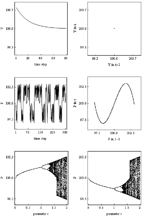
Let us start with Figure 1, which contains the dynamics of isolated goods and stock markets. The top left panel depicts the development of national income, after an exogenous shock in the first period. As already stated in Proposition 1, national income converges monotonically towards its steady-state value. The underlying economic story behind the dynamics is that of the well-known Keynesian multiplier model. After a shock to national income of, say, plus 1 percent, private expenditure and thus national income are b percent above their steady-state values, followed by a positive deviation of b ² percent, and so on, until the shock is completely digested. The top right panel shows the dynamics of national income at time step t versus national income at time step t-1. After a transient phase only a single point remains: the steady-state value of national income. Clearly, without exogenous shocks the goods market dynamics dies out.

+ + + + + Figure 1 about here + + + + +

The center left panel of Figure 1 shows the evolution of the stock price. Since e  1 ,

all steady states of the stock market model are unstable. Instead of a price explosion,

however, intricate bull and bear market dynamics emerge, i.e. erratic up and down

fluctuations in the bull market irregularly alternate with erratic up and down fluctuations in

the bear market. In ( P

, P

₁ ) -space, an S-shaped strange attractor can be detected,

17 indicating that the stock market dynamics is chaotic.

The dynamics of the isolated stock market may be understood as follows. Suppose that the stock market is slightly overvalued. In such a situation, chartists go long and fundamentalists go short. Due to our parameter setting and the fundamentalists’ nonlinear trading rule, excess demand is positive and, as a result, the market maker increases the stock price. Should excess demand still be positive in the next trading period, the market maker quotes an even higher price. Eventually, however, the nonlinearity of the fundamental trading rule kicks in and initiates a change in market powers. Increasingly aggressive fundamentalists render excess demand negative, causing a drop in the stock market.

Afterwards, chartists dominate the market again and the stock price starts to recover. As it turns out, these up and down movements are repeated, albeit in a complex manner.

Occasionally, a bull market turns into bear market. Note that if the stock price is very high, fundamentalists take significant short positions. Excess demand may then be so negative that, due to the market maker’s price adjustment rule, the stock price falls below its fundamental value. In such a situation, chartists turn pessimistic and a period of bear market dynamics sets in. By analogous arguments, a bear market may turn into bull market if the stock price falls very low. Fundamentalists then enter massive long positions, causing a substantial positive excess demand, and thus the market maker is prompted to increase the stock price sharply. Once the stock price exceeds the (perceived) fundamental value, chartists turn optimistic, and their buying behavior starts the next bull market.

The bottom two panels of Figure 1 display two bifurcation diagrams. Here the

dynamics of the stock market is plotted for the chartists’ reaction parameter, ranging from 0

to 2, and two sets of initial conditions. As indicated by Proposition 1, there are three

coexisting steady states and, for e  1 , two of them are locally stable. Initial conditions then

decide whether the stock market is permanently undervalued or overvalued. Our analytical

18

results end at e  1 , yet the bifurcation diagrams show what happens if the chartists’

reaction parameter increases further. As can be seen, two period-two cycles emerge – one located in the bull market and the other in the bear market – each followed by a period-four cycle. A finer resolution would furthermore indicate a sequence of period-doubling bifurcations, leading eventually to complex dynamics, again either located above or below the fundamental value. At around e  1 . 6 , these separated bull and bear market dynamics dissolve and we observe fluctuations similar to those depicted in the central line of panels.

From this point of view, it seems that increasingly aggressive chartists destabilize the underlying economic system.

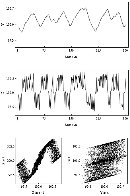
We now investigate the dynamics of the complete model of which Figure 2 provides an example. The first two panels show the course of national income and the stock price, respectively. Irregular fluctuations in economic activity, resembling at least to some degree actual business cycles, coevolve with complex bull and bear market dynamics.

The bottom two panels of Figure 2 illustrate the complexity involved in the dynamics. In the bottom right panel, we plot the stock price at time step t versus the stock price at time step t-1. This panel can be compared with the centre right panel of Figure 1. As we see, the previously S- shaped strange attractor turns into a more complicated, yet still S-shaped object. The bottom right panel of Figure 2 shows the stock price at time step t versus national income at time step t. As to be expected, a strange attractor emerges for the model’s two state variables, also indicating a positive relation between stock prices and national income.

+ + + + + Figure 2 about here + + + + +

3

Recall that the fluctuations of isolated goods market die out over time and that the fluctuations of isolated

stock markets range between 97 and 103 (see Figure 1). In the complete model, however, national income

fluctuates between 99 and 101 while stock price fluctuate between 96 and 104. As mentioned in connection

with Proposition 2, the strength of the bi-directional feedback relation between the real economy and the stock

market may be increased by changing b and c. For instance, for b=0.9 and c=0.07, national income fluctuates

already between 96 and 104 and stock prices between 93 and 107.

19

What drives these dynamics? First of all, the stock price is determined as in the benchmark model, with one crucial exception. Now the (perceived) fundamental value changes over time. Suppose again that the stock price is slightly above the fundamental value so that interactions between chartists and fundamentalists initiate a period of complex bull market dynamics. In contrast to the benchmark model, in which these fluctuations are contained within a certain (constant) range, the range of price fluctuations now shifts gradually upwards. Due to the bull market, private expenditure increases and thus there is an economic expansion. Consequently, speculators perceive a higher fundamental value and therefore the range of the bullish price fluctuations increases. If the stock market eventually crashes, consumption and investment expenditure start to shrink again, sending the economy to a recession. Now speculators perceive comparably lower levels of the fundamental value, which drags the stock market even further down – till a major price correction takes place and the stock market enters the next (temporary) bull regime.

In Figure 3, we explore how the chartists’ and fundamentalists’ reaction parameters affect the dynamics. The left-hand panels show bifurcation diagrams for the stock price and the right-hand panels for national income. The chartists’ reaction parameter varies, as in Figure 1 for the benchmark model, from 0 to 2. Due to multi-stability, two bifurcation diagrams are given for different sets of initial conditions. As stated in Proposition 2, there are three coexisting steady states, two of which are locally stable for

989 . 0 ) 1

/(

) 1

(    

 b b cd

e , as can be seen in Figure 3. Afterwards, a sequence of period-doubling bifurcations emerges, followed first by complex motion restricted to either the bull or the bear market and then ranging across both regions.

A few aspects deserve our attention. First, the steady-state values of the stock prices

are further from P ₁  100 than they are in the benchmark model to P ₁ ^*  100 , as reported in

Proposition 3. However, the same is true for the subsequent regular and irregular dynamics,

20

as long as they are restricted to the bull or bear market regions. Second, for e  1 . 6 , stock prices visit less extreme regions. Of course, stock prices are still highly volatile, but it may be argued that chartists’ high reaction parameters prevent stock prices at least from reaching extreme values. Third, all these phenomena carry over to the goods market. In the benchmark model, there is always a monotonic convergence towards the steady state. In the complete model, there are locally stable steady states, coexisting regular or irregular motions either above or below Y ₁  100 , and complex dynamics fluctuating across bull and bear market regions (this is different to Figure 1, bottom panels, where an increase in chartists’ aggressiveness always increases the amplitude of stock price fluctuations).

Assessing the effect of stock market speculation on national income is not trivial.

Market interactions clearly render the goods market steady state unstable, but national income may, due to a persistent stock market boom, remain permanently above Y ₁  100 . In addition, for e  1 . 6 the evolution of national income is more balanced (i.e. centered around

1  100

Y ) than before. The explanation is rather simple. Most importantly, the adjustment process on the goods market takes time. After the start of a stock market boom, national income improves. However, the adjustment process may be interrupted by a stock market collapse, preventing national income from reaching high values. This is, of course, different to situations where the stock market remains permanently in a bull market. National income and the (perceived) fundamental value then have sufficient time to settle at higher values. In this sense, it is not entirely straightforward whether the economy really benefits from more or less speculative activity.

+ + + + + Figure 3 about here + + + + +

The bottom two panels of Figure 3 present the consequences of an increase in

fundamentalists’ aggressiveness. Since there is no evidence of multi-stability, only one set

of initial conditions is used. As can be seen, the greater the aggressiveness of

21

fundamentalists, the lower the amplitude of business cycles and stock market fluctuations.

In this sense, more aggressive fundamentalists stabilize the dynamics. Nonetheless, fundamentalists are unable to bring the dynamics to a complete rest since the stability of the model’s steady states is independent of parameter f .

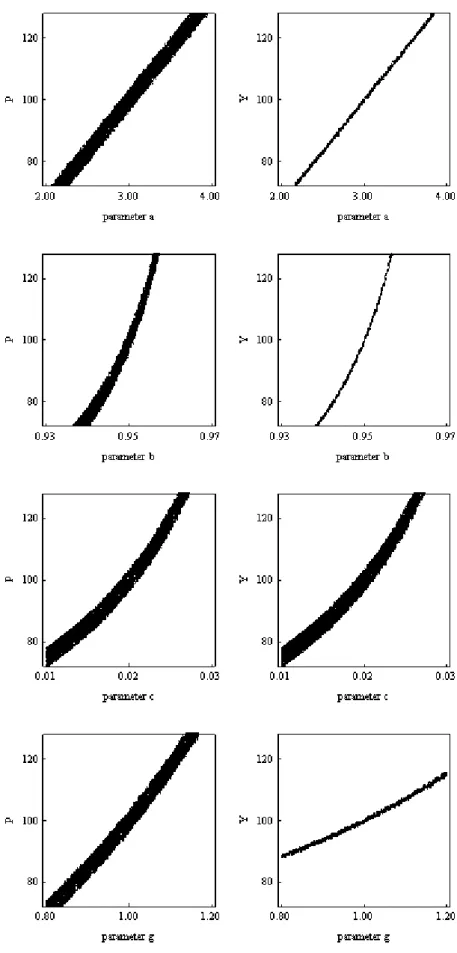
Figure 4 contains bifurcation diagrams for the remaining model parameters. On the left we see results for the stock market and on the right for the goods market. An increase in autonomous expenditures a increases P ₁ and Y ₁ , as evident from Proposition 2, pushing the dynamics upwards. A similar effect is observed for parameters b and c , caused here by a larger multiplier. Finally, an increase in g also stimulates P ₁ and Y ₁ , leading to fluctuations at a higher level. Overall, the dynamics presented in Figure 2 seem to be rather robust since neither a change in a , b , c or d in the selected parameter space of Figure 4 destroys the emergence of endogenous dynamics.

+ + + + + Figure 4 about here + + + + +

5 Conclusions

So far, the main focus of agent-based financial market models is on the dynamics of

financial markets and (virtually) nothing is said about how the dynamics of financial

markets impacts on the real economy and, likewise, how changes in the real economy affect

financial markets. In this paper, we therefore propose a simple behavioral macro model,

enabling us to explore at least some feedback causalities between the real economy and the

stock market. The real economy is approximated by a Keynesian type goods market model

in which consumption and investment expenditure depend on national income and the

performance of the stock market – which links the stock market with the real economy. Our

nonlinear stock market approach explicitly recognizes the trading activity of heterogeneous

speculators, chartists and fundamentalists. Since the fundamental value of the stock market

22

is related to national income, the real economy is linked to the stock market. Ultimately, this establishes a bi-directional feedback structure between the real economy and the stock market and a first starting point for studying interactions between these two economic subsystems.

As it turns out, national income and stock prices are jointly determined by a two- dimensional nonlinear map. The model has three coexisting steady states. The inner steady state, in which national income corresponds to the well-known Keynesian multiplier solution and the stock price to its true fundamental value, is unstable. The two other steady states, located around the inner steady state, are locally stable as long as the chartists’

trading intensity is not too high. Initial conditions then decide whether the economy will enter a permanent boom or a permanent recession. The first scenario is associated with a stock market boom in which stock prices exceed their fundamental value. In the second scenario, the stock market is in a crisis and stock prices fall below the fundamental value. If the local stability of the steady states is destroyed by too aggressive chartists, we observe the emergence of two coexisting period-two cycles, followed by two coexisting period-four cycles, and so on, until there are two coexisting regimes with complex dynamics, either located at a low or high national income and stock price level. If chartists become even more aggressive, we observe intricate switches between bull and bear stock market dynamics, which may then trigger fluctuations in economic activity. Overall, interactions between the real economy and the stock market appear to be destabilizing. This becomes particularly clear if our model is compared which a benchmark model in which interactions are ruled out. Then the unique steady state of the real economy is globally stable, and the stability condition for the two locally stable stock market steady states is less strict.

Given that our model is extremely simple, it may be extended in various directions.

For instance, the case may be considered that the central bank conducts active monetary

23

policy by adjusting the interest rate to influence private expenditure, national income and,

more indirectly, the stock market. Similarly, the case could be considered that the

government relies on countercyclical fiscal policy rules to stabilize the economy. Another

direction to extend our model could be to enrich the goods market. For instance, an

accelerator term could be added to the investment function. Preliminary numerical evidence

reveals that the goods market may then, at least temporarily, decouple from the evolution of

the stock market. Alternatively, one may assume that consumer and investor expenditure are

subject to their sentiments. Then one would obtain a model with animal spirits in the goods

market and stock market. Moreover, a time step in the goods market part of our model

currently corresponds to a time step in the stock market part of the model. One extension of

our model could be to allow for a higher trading frequency in the stock market. Note also

that speculators in our model do not switch between trading strategies. This may be

modified by introducing switching dynamics into the model. For instance, a speculator’s

choice of a trading rule may depend on the rules’ past fitness. Of course, our model could be

developed in various other dimensions. Here we have proposed a rather simple model to

improve our basic understanding of interactions between the real economy and the stock

market. We hope our paper will motivate others to undertake more work in this important

research direction.

24 References

Akerlof, G. and Shiller, R. (2008): Animal spirits. Princeton University Press, Princeton.

Asada, T., Chiarella, C., Flaschel, P., Mouakil, T., Proaño, C.R. and W. Semmler (2010):

Stabilizing an unstable economy: on the choice of proper policy measures. Economics:

The Open-Access, Open-Assessment E-Journal, 4, 2010-21.

Bask, M. (2011), Asset price misalignments and monetary policy. International Journal of Finance and Economics, in press.

Blanchard, O. J., 2009. Macroeconomics, 5th ed. Prentice Hall, New Jersey.

Boswijk, P., Hommes, C. and Manzan, S. (2007): Behavioral heterogeneity in stock prices.

Journal of Economic Dynamics and Control 31, 1938-1970.

Charpe, M., Flaschel, P., Hartmann, F. and Proaño, C.R. (2011): Stabilizing an unstable economy: fiscal and monetary policy, stocks, and the term structure of interest rates.

Economic Modelling, 28 , 2129-2136.

Chiarella, C., Dieci, R. and He, X.-Z. (2009): Heterogeneity, market mechanisms, and asset price dynamics. In: Hens, T. and Schenk-Hoppé, K.R. (eds.): Handbook of Financial Markets: Dynamics and Evolution. North-Holland, Amsterdam, 277-344.

Day, R. and Huang, W. (1990): Bulls, bears and market sheep. Journal of Economic Behavior and Organization, 14, 299-329.

De Grauwe, P. and Kaltwasser, P. (2011): Animal spirits in the foreign exchange market.

Working Paper, University of Leuven.

Dieci, R. and Westerhoff, F. (2010): Heterogeneous speculators, endogenous fluctuations and interacting markets: a model of stock prices and exchange rates. Journal of Economic Dynamics and Control, 34, 743-764.

Franke, R. and Westerhoff, F. (2011): Structural stochastic volatility in asset pricing dynamics: estimation and model contest. Journal of Economic Dynamics and Control, in press.

Galbraith, J. (1997): The Great Crash: 1929. Houghton Mifflin, New York.

Gandolfo, G. (2009): Economic Dynamics, 4th ed. Springer-Verlag, Berlin.

Hommes, C. (2011): The heterogeneous expectations hypothesis: Some evidence from the lab. Journal of Economic Dynamics and Control, 35, 1-24.

Hommes, C. and Wagener, F. (2009): Complex evolutionary systems in behavioral finance.

25

In: Hens, T. and Schenk-Hoppé, K.R. (eds.): Handbook of Financial Markets: Dynamics and Evolution. North-Holland, Amsterdam, 217-276.

Hommes, C., Huang, H. and Wang, D. (2005): A robust rational route to randomness in a simple asset pricing model. Journal of Economic Dynamics and Control 29, 1043-1072.

Kindleberger, C. and Aliber, R. (2005): Manias, panics, and crashes: a history of financial crises, 5th ed. Wiley, Hoboken.

Lengnick, M. and Wohltmann, H. W. (2011): Agent-based financial markets and New Keynesian macroeconomics: a synthesis (updated version). University of Kiel, Economics Working Paper 2011-09.

Lux, T. (2009): Stochastic behavioural asset-pricing models and the stylized facts. In: Hens, T. and Schenk-Hoppé, K.R. (eds.): Handbook of Financial Markets: Dynamics and Evolution. North-Holland, Amsterdam, 161-216.

Lux, T. (1995): Herd behavior, bubbles and crashes. Economic Journal 105, 881-896.

Medio, A. and Lines, M. (2001): Nonlinear Dynamics: A Primer. Cambridge University Press, Cambridge.

Menkhoff, L. and Taylor, M. (2007): The obstinate passion of foreign exchange professionals: technical analysis. Journal of Economic Literature, 45, 936-972.

Minsky, H. (2008): Stabilizing an unstable economy. McGraw-Hill, New York.

Reinhart, C. and Rogoff, K. (2009): This time is different: eight centuries of financial folly.

Princeton University Press, Princeton.

Samuelson P. (1939): Interactions between the multiplier analysis and the principle of acceleration. Review of Economic Statistics, 21, 75-78.

Scheffknecht, L. and Geiger, F. (2011): A behavioral macroeconomic model with endogenous boom-bust cycles and leverage dynamics. Discussion Paper 37-2011, University of Hohenheim.

Tramontana, F., Gardini, L., Dieci, R. and Westerhoff, F. (2009): The emergence of "bull and bear" dynamics in a nonlinear model of interacting markets. Discrete Dynamics in Nature and Society, Vol. 2009, Article ID 310471.

Westerhoff, F. (2009): Exchange rate dynamics: A nonlinear survey. In: Rosser, J.B., Jr.

(ed): Handbook of Research on Complexity. Edward Elgar, Cheltenham, 287-325.

26 Appendix A: Isolated goods and stock markets

Let us start with the goods market. From (1) to (3) we have

t t

t

a bY c P

Y

₁    . (A1)

To isolate the goods market from the stock market, we keep the stock price constant, i.e. we set P

 P ~ . National income is then due to a one-dimensional linear map

P c bY a

Y

~

1   



. (A2) Next, inserting Y

₁  Y

 Y ^* into (A2) reveals that (A2) has the unique steady state

b P c Y a



  1

* ~ . (A3)

Since 0  b  1 , steady state (A3) is obviously positive and globally stable. Moreover, only monotonic adjustment paths are possible.

Let us now turn to the stock market. Combining (4) to (7) yields

1

(

) (

) 3

t

P e P dY f dY P

P

     . (A4)

The stock market is decoupled from the goods market by fixing Y

 Y ~ . We then obtain the one-dimensional nonlinear map

1

(

~ ) ( ~

) 3

t

P e P d Y f d Y P

P

     . (A5)

Setting P

₁  P

 P ^* reveals that Y

d P _* ~

1  , (A6)

and

f e P

P ₂ ^* _{, 3}  ₁ ^*  / , (A7)

i.e. (A5) has three coexisting steady states. Note that P ₂ ^* _{, 3}  0 requires d Y ~  e / f , which

can always be fulfilled by shifting Y ~ sufficiently upwards.

27

A steady state of a one-dimensional nonlinear map is locally stable if the slope of the map, evaluated at the steady state, is smaller than one in modulus. Since the slope of the map at P ₁ ^* is equal to 1  e , steady state P ₁ ^* is unstable. The slope of the map at steady states P ₂ ^* _{, 3} is 1  2 e . Hence, steady states P ₂ ^* _{, 3} are locally stable for

1

e  . (A8) For a deeper analysis of map (A5) see Tramontana et al. (2009).

Appendix B: Interacting goods and stock markets

From (A1) and (A5) it follows directly that the dynamics of the complete model is due to the two-dimensional nonlinear map



 























1 3 1

) (

)

(

t t

t t t

P dY f dY P e P P

cP bY a

Y . (B1)

Plugging Y

₁  Y

 Y and P

₁  P

 P into (B1), we find that the model has three coexisting steady states

b P c a cd b Y a



 



 

1

1 ¹

1 , _{1 1}

1 d Y

cd b

P ad 



  (B2)

and

f e cd b Y c

Y    

1 1

3 ,

2 ,

f e cd b P b

P  

 

 1

1 1

3 ,

2 . (B3)

Obviously, Y ₁  0 requires b  cd  1 . Moreover, Y _{2 , 3}  0 and P _{2 , 3}  0 needs a  c e / f and ad  ( 1  b ) e / f , respectively. To ensure that the model’s steady states are positive, we thus assume that b  cd  1 and that a is sufficiently large.

The Jacobian matrix at steady state ( Y ₁ , P ₁ ) is given by

28

 

 







 

e ed

c P b

Y

J ₁ ( ₁ , ₁ ) 1 , (B4)

with determinant d et ( J

)  b  be  cde and trace tr ( J

)  1  b  e . Local stability of the steady state ( Y

, P

) would necessitate that

0 2

2 ) ( ) (

1  tr J

 d et J

  b  e  be  cde  , (B5a) 0

) 1 (

) ( ) (

1  tr J

 d et J

 e b  cd   , (B5b) 0

1 ) (

1  d et J

  b  be  cde  . (B5c) Since b  cd  1 , inequality (B5b) is never true, i.e. the steady state ( Y

, P

) is unstable.

The Jacobian matrix at steady states ( Y

, P

) reads

 

 





 

e de

c P b

Y

J

(

,

) 2 1 2 , (B6)

with determinant d et ( J

)  b  2 be  2 cde and trace tr ( J

)  1  b  2 e . Hence, local stability of steady states ( Y

, P

) is guaranteed if

0 2

2 2 2 2 ) ( ) (

1  tr J

 d et J

  b  e  be  cde  , (B7a) 0

) 1

( ) ( ) (

1  tr J _{2 , 3}  d et J _{2 , 3}  e  b  cd  , (B7b) 0

2 2 1 ) (

1  d et J

  b  be  cde  . (B7c) While inequalities (B7b) and (B7c) always hold, inequality (B7a) is only satisfied if

cd b e b





  1

1 . (B8)

An introduction to nonlinear dynamical systems, including a stability analysis of their

steady states, can be found in Gandolfo (2009) and Medio and Lines (2001), for instance.

29

Figure 1: The dynamics of isolated goods and stock markets.

Parameter setting as in Section 4. Bifurcation parameters as indicated on the axis.

30

Figure 2: The dynamics of interacting goods and stock markets.

Parameter setting as in Section 4.

31

Figure 3: Speculative forces and the dynamics of the complete model.

Parameter setting as in Section 4. Bifurcation parameters as indicated on the axis.

32

Figure 4: Real forces and the dynamics of the complete model.

Parameter setting as in Section 4. Bifurcation parameters as indicated on the axis.