Quit Turnover and the Business Cycle: A Survey.

IHS Economics Series Working Paper 317

October 2015

Quit Turnover and the Business Cycle: A Survey.

Carlos Carrillo-Tudela

Melvyn Coles

Impressum Author(s):

Carlos Carrillo-Tudela, Melvyn Coles Title:

Quit Turnover and the Business Cycle: A Survey.

ISSN: Unspecified

2015 Institut für Höhere Studien - Institute for Advanced Studies (IHS) Josefstädter Straße 39, A-1080 Wien

E-Mail: o ce@ihs.ac.atffi Web: ww w .ihs.ac. a t

All IHS Working Papers are available online: http://irihs. ihs. ac.at/view/ihs_series/

This paper is available for download without charge at:

https://irihs.ihs.ac.at/id/eprint/3699/

Quit Turnover and the Business Cycle: A Survey.

Carlos Carrillo-Tudela

University of Essex, CEPR, CESifo and IZA

Melvyn Coles

University of Essex

June 2015

1 Introduction

Workers might change jobs for many reasons. They might fall out with the boss and so decide to change employer, or learn that the job is not really for them, or they might accept a poorly paid job as being preferable to being unemployed - say gathering work experience improves one’s CV - and continue search for something better while employed. A slightly different reason is that some firms may hit a sticky patch and, fearing the risk of layoff, employees quit to more permanent employment elsewhere. A competitive labor market ensures such quit turnover is efficient: it reallocates workers from less to more productive matches. In non-competitive labor markets, however, firms always have the incentive to increase profit by paying a wage below marginal product while, in the absence of slavery contracts, employees always retain the option of quitting to better paid employment. The interaction between these two forces need not generate efficient outcomes. The focus of this chapter is to consider new developments in the search and matching literature where wages, quit turnover and unemployment are endogenously determined in economies with aggregate shocks. The aim of the discussion is not only to highlight possible market failures but also to explain how on-the-job search and employee turnover fundamentally affect our understanding of fluctuations in aggregate employment.

∗Correspondence: Department of Economics, University of Essex, Wivenhoe Park, Colchester, CO4 3SQ, UK. Email: cocarr@essex.ac.uk.

†Corresponding author: Department of Economics, University of Essex, Wivenhoe Park, Colchester, CO4 3SQ, UK. Email: mcoles@essex.ac.uk.

1For a wider survey of the on-the-job search literature see Mortensen (2003), Manning (2003). More recently Hornstein et al. (2011) ask whether job search models can explain the large amount of wage dispersion in the data and conclude that on-the-job search plays an important role in explaining such

21000   22000   23000   24000   25000   26000   27000   28000   29000  

1200   1300   1400   1500   1600   1700   1800   1900   2000  

1993q1   1993q4   1994q3   1995q2   1996q1   1996q4   1997q3   1998q2   1999q1   1999q4   2000q3   2001q2   2002q1   2002q4   2003q3   2004q2   2005q1   2005q4   2006q3   2007q2   2008q1   2008q4   2009q3   2010q2   2011q1   2011q4   2012q3   2013q2  

Hires   Separa5ons   Employment  

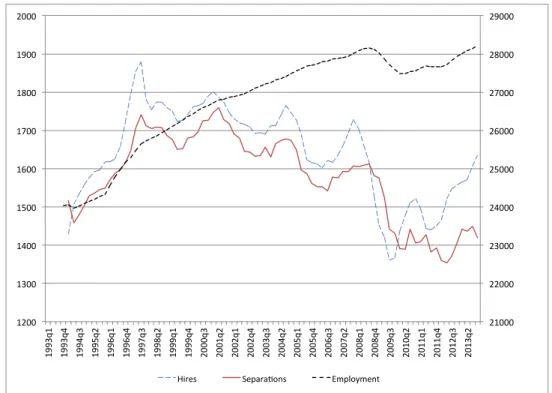
Figure 1: Gross hires, job separations and employment in the UK: 1993-2013 We begin with some motivating evidence. Gross hire flows and gross job separation flows are large, volatile and dwarf the relatively small (net) changes in employment. Using quarterly data, Figure 1 describes how (i) gross hires, (ii) gross job separations and (iii) total employment evolved in the U.K. over the period 1993-2013. All series are drawn to the same scale (thousands of workers) where the left scale describes the gross quarterly flows while the right scale describes total UK employment.

An economy with full employment would find gross hires and gross separations per- fectly overlap. Instead with less than full employment, employment increases whenever gross hires exceed gross job separations. The central feature of these data, however, is that gross job hires and gross job separations vary widely over the cycle, though the two time series track each other so that the gap between them is always small. For example the 2008-2009 recession was associated with an alarming 20% drop in gross hires. Unem- ployment grew strongly during this phase for separations exceeded hires, but the steep fall in hires was closely matched by a steep fall in job separations resulting in a decline

data. When in addition there is learning-by-doing, the framework is easily consistent with the data;

interesting papers using this extended approach include Burdett et al. (2011, 2015), Bagger et al. (2014).

Other important developments use the on-the-job search framework to identify wages and equilibrium sorting, see for example Eeckhout and Kircher (2011), Hagedorn et al. (2014), Lamadon et al. (2014).

Such work, however, is beyond the remit of this chapter.

2We use the U.K. Labour Force Survey to construct the time series reported in the figure. These series are smoothed using a 4 quarter moving average.

in employment which was (relatively) modest.

So why do gross hires and gross separations track each other so closely? The answer is that quit turnover is both large and endogenous. For example, we find that on average 42% of the quarterly hires reported in Figure 1 are filled by job-to-job transitions (see also Fallick and Fleishman (2004) for similar evidence using U.S. data). Thus when gross hires increase in a boom, so does quit turnover. A competitive framework explains such turnover as a creative/destruction process: as new high productivity jobs come on the market, the competitive process drives up the market-clearing wage and workers quit (or separate) from low productivity firms to the new, more productive ones. Monopsony equilibrium with less than full employment instead implies quit turnover increases in the recovery simply because there are more jobs available on the market and, just like the unemployed who wish to escape a low income state, so do workers in low wage employment. The key issue then is understanding the nature of quit turnover and unemployment over the cycle.

Figure 1 does not distinguish between separations due to job destruction shocks (where laid-off workers enter unemployment), or separations where an employee simply quits to take preferred employment elsewhere. Table 1 describes for the U.K. how the job finding hazard rates of the unemployed (h

), job-to-job hazard rates of the employed (h

) and separation hazard rates of the employed into unemployment (h

) covary with measures of worker productivity, unemployment and GDP.

Table 1: Cyclical Correlations

Raw correlations Unemployment GDP Productivity h

(re-employment rates) -0.44 0.47 0.43

h

(job-to-job quits) -0.61 0.76 0.76

h

(job-to-unemployment) 0.28 -0.53 -0.62

Table 1 reveals that hazard rates into unemployment [h

] are strongly countercyclical:

recessions are characterised by many more employed workers entering unemployment. In contrast, unemployed worker re-employment rates [h

] and employed worker job-to-job transition rates [h

] are strongly procyclical (and highly correlated with each other).

Burdett (1978) and Burdett and Mortensen (1998) [BM from now on] are the key seminal papers on endogenous quit turnover in non-competitive labor markets. Given an exogenous distribution of wage offers by firms, Burdett (1978) shows how on-the-job

3The table is constructed using the U.K. LFS for the period 1991-2012, whereh^{U E} is measured as the ratio between the flow of workers that were unemployed in quartertand transited to employment in quartert+ 1 and the stock of unemployed workers in quartert; i.e. h^{U E}_t =U Et+1/Ut. We measureh^EU andh^EE in similar ways but based on the stock of employed workers. Worker productivity is measured using output per worker. The correlations shown in the table are computed using the cyclical components of the log of each of these series using an HP filter with a smoothing parameter value of 1600.

search generates a worker wage profile which, in expectation, is an increasing, concave function of age. The wage profile is increasing (in expectation) as each time the worker receives a better outside offer the worker quits to take the better paid post. The wage profile is concave for each time the worker quits to take a better paid position, the worker, in the future, is less likely to find an even better paid position. Thus a worker’s quit rate also declines (on average) with age. Furthermore workers fear being laid-off as they will, once more, have to climb the wage ladder starting from the bottom rung. In a most elegant way, on-the-job search captures many features of the labor market experience.

BM extend those insights to an equilibrium framework where firms which pay higher wages enjoy lower quit rates and attract more hires. This chapter examines the recent literature which further extends that approach to aggregate shocks and costly hiring. The former extension is important for job-to-job quits are highly procyclical and so likely to have a direct impact on (cyclical) unemployment. The second is important for it is key to understanding how non-competitive hiring and quit turnover distorts unemployment and so identifies genuine policy issues.

In the absence of slavery contracts, an important issue is what type of employment contract should a firm offer? Stevens (2004) provides an excellent analysis of the set of first best contracts when there is on-the-job search with risk neutral workers.

One optimal contract is that a new hire buys the job - the worker pays a job fee f > 0 - and signs an employment contract where the firm promises to pay marginal product in the entire future. Menzio and Shi (2011) adopt this simple contract structure in a directed search framework with idiosyncratic match payoffs. The resulting analysis is “close” to the competitive paradigm in that it finds the allocation of resources, and unemployment in particular, is efficient. It provides an excellent first step in understanding how a quasi- competitive economy with frictional unemployment and endogenous quit turnover reacts to aggregate shocks. We examine those insights in detail below.

A different optimal contract is that the terms of trade are determined by Bertrand competition when a worker receives an outside offer (e.g. Postel-Vinay and Robin (2002)).

As long as there is no endogenous job search effort (otherwise employees chase outside of- fers to get a pay increase - see Postel-Vinay and Robin (2004) for example), quit turnover is again jointly efficient. Robin (2011) extends that case to aggregate productivity shocks, though with no costly hiring margin. Lise and Robin (2015) further extend that approach by introducing a competitive vacancy market. It turns out this sequential auction ap- proach is remarkably flexible and useful for structural estimation. We also describe this

4We do not consider here contracts which increase wages with seniority and so reduce worker quit rates by rewarding loyalty. See Burdett and Coles (2003), Shi (2009), Lentz (2014) for the analysis of optimal wage-tenure contracts with equilibrium job search and risk averse workers.

framework in detail below.

A very different approach, however, instead supposes labor contracts are not first best.

Job fees are rarely (if ever) observed in the labour market (presumably the real world issue is that it is not possible to verifiably measure a worker’s marginal product). Although university chancellors might consider matching outside offers in academia, it is not clear that Bertrand competition is widespread practice in other occupations. We use dynamic monopsony here to refer to the case of equal treatment: that a firm must pay the same wage to equally productive workers doing the same job regardless of race, gender, sex- uality, etc. Thus should an employee on the factory floor receive an outside offer, the firm does not Bertrand compete on that worker’s wages (the sequential auction approach presumes perfect wage discrimination). Rather the worker is allowed to quit to the pre- ferred employment opportunity and the firm considers whether to hire a replacement at the company wage.

As is well known, non-competitive price setting with no price discrimination generates economic inefficiencies. The classic textbook case argues a monopsonist increases profit by lowering its wage along the labour supply curve. With dynamic monopsony as considered here, however, the market inefficiency is more subtle. In Coles and Mortensen (2015), equilibrium unemployment is inefficiently high not because firm hiring rates are too low, rather because quit rates are too high and replacing workers who quit is a time consuming process. Or put differently, unless and until a firm replaces a worker who quits, a job to job transition implies a job is destroyed at the previous employer. Not surprisingly, excessive job destruction rates generate too high unemployment.

Unfortunately describing stochastic equilibria with dynamic monopsony and costly hiring is complex. The Menzio and Shi (2011) and Lise and Robin (2015) approaches are tractable for they assume efficient contracts, a zero profit condition for vacancy creation and a constant returns to scale matching technology. As is standard in the DMP frame- work without on-the-job search, this generates a very special result - that equilibrium values are independent of unemployment. The free entry assumption, however, is clearly strong. Unfortunately any other hiring cost technology requires identifying the optimal hiring strategy of each individual firm given the quit strategies of its employees which, in turn, depend on the entire set of firm hiring strategies. In a stochastic environment, this is a complex fixed point problem.

Moscarini and Postel-Vinay (2013) were the first to extend the dynamic monopsony

framework of Burdett and Mortensen (1998) to the stochastic case. Here we focus on

the Coles and Mortensen (2015) framework which instead assumes hiring costs exhibit

constant returns to scale; that is, a firm with twice as many employees which wishes

to hire twice as many new recruits has twice the hiring costs. The resulting structure generates Gibrat’s Law, that firm growth rates depend on productivity but are otherwise independent of firm size. The simpler structure not only yields a fully tractable macro- equilibrium, the model is extended to allow firm turnover with entry by new start-up companies and idiosyncratic firm productivity shocks.

After quickly describing the BM framework, the following describes and discusses these stochastic extensions. The conclusion describes the insights learned from these approaches.

2 The BM Paradigm

Time is continuous, denoted t

[0,

neutral, equally productive, infinitely lived and discount the future at rate r > 0. At any point in time, each worker is either (i) employed earning some wage w, (ii) unemployed with home production b

0. We let U denote the unemployment rate.

There is a unit measure of firms indexed by x

U[0, 1], where each firm x is risk neutral with productivity p(x) > b and p(.) is an increasing function. There are constant returns to scale: a firm with n employees generates flow revenue np(x). There is exogenous job destruction: at rate δ > 0 an employee at firm x separates and enters unemployment.

There are no hiring costs and all workers receive job offers at an exogenous rate:

unemployed workers receive jobs offers at rate λ

, while employed workers receive job offers at rate λ

. The data suggest λ

< λ

as unemployed worker re-employment rates are much greater than employed worker job-to-job transition rates.

In steady state (below we extend to non-steady state), each firm x precommits to a fixed wage w = w(x) which it pays to each employee. Corresponding to these wage strategies w(.) is a distribution of wage offers F (.). BM show this distribution, in equilibrium, is continuous (no mass points) and has connected support. For ease of exposition we simply assume F (.) has these properties. As the wage paid is fixed, if an employee receives an outside job offer at wage w

> w, the worker accepts the job offer and quits. Once a worker rejects a job, there is no recall.

A key object is the employment distribution G(x), where 1

G(x) is the measure of workers who are employed in firms with type greater than x. Identifying equilibrium takes two steps. As workers do not care about the firm’s type x, only the wage w that it pays, the first step is to describe the optimal job search strategies of workers. This is very

5In the UK, for example, using the LFS for the period 1991-2012 we find that the average quarterly value of h^{U E} is 0.26, while the average quarterly value of h^EE is 0.026.

simple. The second step is to describe the equilibrium wage strategies of firms x

[0, 1]

given the reservation wage R of unemployed workers and that on-the-job search implies employed workers will quit if offered a better paid job.

2.1 Reservation wage strategies in BM

Standard arguments imply, with random contacts, that the flow value of being unemployed satisfies the Bellman equation

rV

= b + λ

w

max[V

(w

)

V

, 0]dF (w

), where V

(w) is the value of being employed on wage w and satisfies

(r + δ)V

(w) = w + λ

w

max[V

(w

)

V

(w), 0]dF (w

) + δV

.

As V

must be increasing in the wage paid w [it is better to earn a higher wage], an unemployed worker accepts any job offer with wage w

R where V

(R) = V

. Putting w = R in the above and solving identifies the reservation wage equation:

R = b + (λ

λ

)

R

[V

(w)

V

]dF (w). (1)

Equation (1) identifies an important tension in this literature. The case λ

> λ

assumes unemployed workers have access to a more efficient search technology: taking a job implies a fall in the job offer rate. Unemployed workers thus require wage w

R > b to compensate for foregone search effectiveness. This case would not seem entirely realistic: if anything network effects suggest that already employed workers have better opportunities for accessing outside job offers. If all workers instead have equal access to the same search technology, the reservation wage equation implies R = b (there is no foregone search effectiveness by taking a job) even though unemployed job seekers might choose greater search effort and so enjoy more frequent job offers (e.g. Lise (2013)). Unfortunately we must rule out endogenous job search effort. For ease of exposition we assume λ

= λ

so that R = b, and refer the reader to BM for the extended case. We continue to retain the λ

, λ

distinction, however, as it is useful to distinguish between the two types of job offers.

6WhileV^E(w)≥V^U,otherwise the worker quits into unemployment and obtainsV^U.

2.2 Equilibrium wage strategies in BM

Consider now any firm x

[0, 1]. This firm takes as given the wage strategies w(x) of

firms x

[0, 1] which together determine F . Let G

denote the steady state distribution of earnings across employed workers. For any wage w

R = b, steady state turnover implies G

is given by:

δ[1

G

(w)] = [λ

U + λ

[G

(w)

U]] [1

F (w)],

where the left hand side describes the flow out of workers employed on wage greater than w [through job destruction] which, in steady state, must equal the flow in [which is composed of those unemployed and those employed on a wage below w who receive a wage offer greater than w]. Solving implies

G

(w) = δ + (λ

λ

) [1

F (w)]U

δ + λ

[1

F (w)] . (2)

Suppose now firm x

posts wage w

. If it posts wage w

< R = b it makes zero steady state profit [all workers prefer unemployment]. Suppose it posts wage w

b. In steady state its employment level n

is given by

[λ

[1

F (w

)] + δ] n

= λ

U + λ

[G

(w

)

U ],

where the left hand side describes its outflow of workers (through quits and job destruc- tion), the right hand side describes gross hires (from unemployment and from firms paying lower wages). Solving yields

n(w

) = λ

U + λ

[G

(w

)

U]

λ

[1

F (w

)] + δ . Firm x

thus offers wage w

R to maximise steady state profit:

Ω(x

) = max

w⁰

λ

U + λ

[G

(w

)

U ]

λ

[1

F (w

)] + δ [p(x

)

w

]. (3)

The first order condition describing optimal w

, and thus the optimal wage strategy w =

w(x

), is given by (6) below. The crucial comparative static is that it is optimal for a firm

with greater productivity p = p(x) to post a strictly greater wage. The intuition is simply

that an employee is more valuable to the more productive firm and so the firm is willing to

post a higher wage to attract and retain additional employees. As firm optimality implies

w(.) must be an increasing function, the distribution of wage offers is now determined by

F (w(x)) = x. (4)

A Market Equilibrium

is a set of wage strategies across firms; i.e. w = w(x) for all x

[0, 1], such that:

•

(a) wage distributions F, G

are given by (4), (2) with steady state unemployment U = δ/(λ

+ δ),

•

(b) wage strategies are optimal given F, G

; i.e.

w(x) = arg max

w⁰

λ

U + λ

[G

(w

)

U ]

λ

[1

F (w

)] + δ [p(x)

w

] for all x

[0, 1]. (5) Solving this fixed point problem is easy - see BM for full details. Essentially the necessary first order condition for optimality implies optimal wage:

w(x) = p(x)

[λ

U + λ

[G

(w)

U ]] [λ

[1

F (w)] + δ]

λ

G

(w) [λ

[1

F (w)] + δ] + λ

F

(w) [λ

U + λ

[G

(w)

U ]] (6) where w = w(x). As F (w) = x and G

(w) = G(x) at w = w(x), total differentiation implies

F

(w) = 1

w

(x) , G

(w) = G

(x) w

(x) .

Substituting out these objects in (6) yields the first order differential equation dw

dx = [p(x)

w(x)] λ

G

(x) [λ

[1

x] + δ] + λ

[λ

U + λ

[G(x)

U ]]

[λ

U + λ

[G(x)

U]] [λ

[1

x] + δ] . (7) where steady state

G(x) = δ + (λ

λ

) [1

x]U

δ + λ

[1

x] . (8)

Equilibrium w(.) is thus the solution to the first order differential equation (7) with G given by (8) and initial value w(0) = b. It is easy to show the solution implies w(x) < p(x) [i.e. firms pay wage below marginal product] and dw/dx > 0 [more productive firms pay higher wages]. To reveal the underlying wage structure, however, let q(x) denote the equilibrium quit rate at firm x; i.e.

q(x) = λ

[1

x],

and so q

(x) =

is the marginal quit rate. Let H(x) denote its equilibrium hiring rate;

i.e.

H(x) = λ

U + λ

(G(x)

U ),

and so H

(x) = λ

G

(x) is the marginal hire rate. Substituting out λ

, λ

in the wage equation (7) identifies the monopsony wage condition:

dw

dx = [p(x)

w(x)]

H

(x)

H(x)

q

(x) q(x) + δ

. (9)

Along the equilibrium wage profile w = w(.), each firm x increases its wage offer w to its equilibrium wage w(x) for it is at this point the marginal cost of paying a higher wage to current employees exactly equals its marginal return, which is the firm’s profit stream p(x)

w per employee multiplied by the marginal increase in labor supply (by hiring more recruits and reducing employee quit rates). At wages w < w(x), increasing wage increases profit by attracting more workers and reducing worker quit rates, while for w > w(x) the latter return is sufficiently small it is better to pay a lower wage.

Allowing job fees completely changes the equilibrium structure. Suppose for example firms are equally productive (i.e. p(.) = p) and can charge job fees f. Optimal contracting in the above implies each firm pays marginal product w = p and sets job fee f = [p

b](r + δ). Such an equilibrium implies no job-to-job transitions [workers are paid marginal product] and the job fee extracts full surplus from unemployed workers (who have V

= b/r).

Sequential auctions also completely change the equilibrium structure. Again suppose identical firms and note Bertrand competition implies an employee earns marginal product w = p on receiving an outside offer. As firms post offers and so extract full surplus from unemployed workers, each new recruit when hired from unemployment is offered starting wage

w

= b

λ

p

b r + δ

,

which reflects at rate λ

the worker enjoys a pay rise to wage w = p by getting an outside

offer. In this special case the sequential auction approach is payoff equivalent to the job

fees case: turnover is efficient, full surplus is extracted from unemployed workers. The

only difference is that rather than pay an upfront job fee f, the new recruit with sequential

auctions earns low starting wage w

< p until a job offer is received.

3 The Stochastic Extensions.

There are three key approaches to the stochastic case with costly hiring. The following discusses in turn Menzio and Shi (2011) [job fees and directed search], Lise and Robin (2015) [sequential auctions] and Coles and Mortensen (2015) [dynamic monopsony]. To keep notation consistent across sections, this survey uses θ to denote aggregate produc- tivity and so uses φ to describe market tightness.

3.1 Job Fees and Directed Search - Menzio and Shi (2011)

Menzio and Shi (2011) assume firms are ex-ante identical but extend the BM approach by allowing idiosyncratic match values and aggregate shocks. The critical ingredients are it allows jobs fees and that on-the-job search is directed. The reader who does not know well the directed search approach might first read the useful survey by Rogerson et al.

(2005).

All workers are ex-ante identical as are firms. There are constant returns to matching and free entry of vacancies. As the size of a firm is not well defined, consider a one firm/one job technology where given aggregate productivity θ

, .., θ

and match productivity z

Z =

, .., z

flow output of the match is θ + z. Assuming discrete time, θ follows a Markov chain with transition probabilities described by H(θ

When a job match is formed, the match specific component z is considered a random draw from distribution F (.) and is fixed during the lifetime of the match. We focus here on the more interesting case that the worker learns the match value z only once the job has been accepted.

Matching takes place on islands where, given market tightness φ on a given island (consistent with a free entry rule), a worker on that island contacts a vacancy with prob- ability m(φ), the vacancy is contacted by a worker with probability q(φ), where constant returns to matching implies q(φ) = m(φ)/φ. As is standard, m(.) is assumed strictly concave and increasing in φ.

At the start of each period, Nature chooses a random fraction λ

of the unemployed to be able to search, while a random fraction λ

λ

of employed workers are able to search. As is standard in the directed search framework, workers in different employment states will search on different islands.

Consider those employed workers in employment state (z, θ) who, in equilibrium, seek

employment on island (z, θ). With job fees, firms with vacancies on this island offer

an equilibrium job fee f

and a contract which promises to pay wage equal to realised

marginal product in the entire future while the match survives. With free entry, let

φ

0 describe the equilibrium market tightness on this island (where φ

= 0 if it is not an equilibrium that an employed worker with match value z searches for a new job).

If W

(z, θ) is the equilibrium value of being employed in state (z, θ) on a contract which always pays marginal product, then

W

(z, θ) = max







b+βEθWu(θ⁰), δ[b+βE_θW_u(θ⁰)] + (1−δ)

( [1−λ1m(φ_zθ)] [θ+z+βE_θWe(z, θ⁰)]

+λ₁m(φ_zθ){−f_zθ+E_z⁰[θ+z⁰+βE_θW_e(z⁰, θ⁰)]}

)







,

with discount factor β

(0, 1) and δ > 0 is the probability of (exogenous) job destruction.

The first line describes the worker’s option to quit into unemployment where W

(θ

) is the value of being unemployed in aggregate state θ

. If the job is not destroyed then with probability λ

m(φ

) an employed worker in state (z, θ) receives a job offer. After paying the posted job fee f

, the worker begins employment with new realised match value z

, where a no recall assumption implies the worker cannot go back to his/her previous job if realised z

< z. Free entry implies the zero profit condition

k = q(φ

)f

where k > 0 is the per period cost of holding an open vacancy and the job fee f

is the firm’s profit by filling it.

A directed search equilibrium determines the equilibrium job fee f

and market tight- ness φ

. Menzio and Shi (2011) formally establish that the unique directed search equi- librium implies (f

, φ

) maximises worker value; i.e.

W

(z, θ) = max

f,φ≥0







b+βE_θWu(θ⁰), δ[b+βEθWu(θ⁰)] + (1−δ)

( [1−λ₁m(φ)] [θ+z+βE_θW_e(z, θ⁰)]

+λ₁m(φ){−f+E_z⁰[θ+z⁰+βE_θW_e(z⁰, θ⁰)]}

)







subject to the zero profit condition:

k = q(φ)f.

The argument is intuitive: suppose equilibrium implies any other market pair (f

, φ

)

satisfying zero profit and so employed workers enjoy suboptimal market value W

. With

free entry, firms then have the incentive to deviate to an alternative matching island, one

which offers the welfare maximising fee f

. Employed workers in market (f

, φ

) with

market value W

queue on this alternative island with a market tightness φ

φ

which

leaves them indifferent between search on the two islands. Straightforward algebra finds that deviating firms on the island offering f

make strictly positive expected profit; i.e.

a profitable deviation exists and so (f

, φ

) cannot describe equilibrium.

Using the zero profit condition to substitute out f yields the recursive Bellman equa- tion:

W

(z, θ) = max

φ≥0







b+βEθWu(θ⁰), δ[b+βE_θW_u(θ⁰)] + (1−δ)

( −λ_ekφ+ [1−λ1m(φ)] [θ+z+βE_θWe(z, θ⁰)]

+λ₁m(φ)E_z⁰[θ+z⁰+βE_θW_e(z⁰, θ⁰)]

)







.

The crucial simplification is the equilibrium island outcome (φ

, f

) for each market type (z, θ) is independent of aggregate unemployment and the distribution of match values across employed workers. Simple value function iteration thus immediately identifies the worker value functions W

(.) and corresponding job-to-job transition rates λ

m(φ

) which vary by match value z and the aggregate productivity state θ. There is also endogenous job destruction: given aggregate productivity θ, workers quit into unemployment if match value z

R(θ) where W

(R, θ) = W

(θ).

The model is easily calibrated to the data, the novel feature being that the distribution of match values F (.) is calibrated so that worker tenures in the model are consistent with the empirical distribution of tenures across employed workers. As the cost k of a vacancy is held fixed, a favourable productivity shock reduces the relative cost k/θ of re-allocating workers. The calibrated model finds a positive aggregate productivity shock unambigu- ously increases unemployed worker job finding rates and so h

is strongly procyclical.

It also raises job-to-job transition rates in poor job matches (z low), thus there is greater re-sorting when productivity is high. Although job-to-job transition rates decrease in higher z matches, the average job-to-job transition rate h

is highly procyclical.

Perhaps the most interesting result is that the model captures a large part of the un- employment volatility observed in the data. The insight is the calibration finds there is a high density of marginal jobs, those whose match values z lie close to the job destruction threshold R(θ). Thus in good times where R(θ) is low, many low z−jobs accumulate over time. An adverse aggregate productivity shock then causes these jobs to be de- stroyed: workers optimally separate from these low z−jobs into unemployment. Thus small productivity shocks can generate large variations in unemployment. Mortensen and Pissarides (1994) tells a similar story. Shimer (2005) explains why this mechanism cannot play an important role in a standard DMP framework without on-the-job search:

the free entry assumption implies vacancies tend to increase as unemployment increases

(which is strongly counterfactual). Indeed the Menzio and Shi (2011) calibration with

free entry and constant returns to matching continues to imply “vacancies directed to the unemployed” increase in the recession. This is a little problematic for, if there were ever such a thing as “vacancies directed to the unemployed”, vacancies posted in UK Job Centres would be those. Coles and Smith (1998) find such vacancies fall strongly in recessions. Nevertheless the Menzio/Shi framework finds that “vacancies directed to the employed” fall in a recession and the total effect is that vacancies fall. Although the model does not generate large variation in vacancies over the cycle, it successfully avoids the counterfactual strong positive correlation between unemployment and vacancies.

4 Sequential auctions - Lise and Robin (2015)

Just as in the Menzio and Shi (2011) approach with job fees, the sequential auction approach guarantees efficient separations. An important difference, however, is that un- employed workers and employed workers here chase the same set of vacancies and so crowd out each others’ job finding opportunities. The framework remains highly tractable, how- ever, for it continues to assume constant returns to matching with a competitive vacancy market.

The Lise and Robin (2015) framework also adopts a one firm-one job framework but this time with two sided ex-ante heterogeneity. There is a unit measure of workers, a unit measure of firms and all are infinitely lived. Firms are characterised by a productivity parameter x

U [0, 1], each worker is characterised by a productivity parameter y

[0, 1]

with density l(y). Aggregate productivity shocks are described by θ which evolve each period according to transition matrix H(θ

An unemployed worker y in state θ generates home production b = b(y, θ) and searches for a job with search effectiveness parameter s

> 0. An employed worker y in firm (x, θ) produces output p = p(x, y, θ) and searches on-the-job with search effectiveness parameter s

.

The first key assumption is that, should a worker receive an outside offer, the terms of trade are determined by Bertrand competition. The second is that hiring takes place through a competitive vacancy market. Specifically any unmatched firm x which wishes to hire a worker must first purchase vacancies at period t price c

. As expected profits are linear in the number of vacancies purchased, a competitive equilibrium implies each unmatched firm x must make zero expected profit. The vacancy price c

is determined by the marginal cost of vacancy supply; i.e. c

= c

(v

(x)), where c(.) is strictly convex and v

(x) is the equilibrium number of purchased vacancies.

Matching takes place in a single market, described by a matching function M =

M (L, V ) where L = s

U + s

(1

U ) is total effective search units given unemployment U, and V is total vacancies. Assuming M (.) is homogenous of degree one, let m = M (1, V /L).

Thus an unemployed worker receives a job offer with probability s

m while an employed worker receives a job offer with probability s

m.

Let u

(y) denote the measure of type y workers who are unemployed at date t, h

(x, y) denote the measure of type y workers employed in type x firms. These measures evolve endogenously and are potentially payoff relevant. Let G = (u, h) and so denote the aggregate state space as (θ, G).

As different workers are paid different wages, let Π(w, x, y, θ, G) denote the expected discounted profit of a firm x which employs worker y on current wage w. Let V

(w, x, y, θ, G) denote the worker’s corresponding expected value of employment, while V

(y, θ, G) is the worker’s value of being unemployed in this state. As there is transferable utility, define match surplus:

S(x, y, θ, G) = V

(w, x, y, θ, G) + Π(w, x, y, θ, G)

V

(y, θ, G).

Although S(.) potentially depends on w, and would do so if the wage affected any real outcome, the assumption that wages are renegotiated so that trade is always (jointly) efficient ensures S(.) is independent of w. Also note that if the match were to break up, the worker would enjoy continuation value V

(y, θ, G) while unemployed but the unmatched firm would make zero expected profit in the competitive vacancy market. The focus of the analysis is to characterise the equilibrium surplus function.

Consider first an unemployed worker y who contacts a type x firm with an unfilled job. If the surplus to the match S(x, y, .)

0, a match forms and the worker is employed at a wage which leaves him/her just indifferent to taking the job. The worker y is thus hired at starting wage w = w

(x, y, .), where V

(w

, x, y, .) = V

(y, .). As unemployed workers never obtain any surplus from a job offer, V

is defined recursively by:

V

(y, θ) = b(y, θ) + 1 1 + r E

V

(y, θ

) and so is independent of G.

Consider now a worker y employed at firm x who receives an outside job offer from

firm x

. Suppose S(x

, y, .) > S (x, y, .) and so it is efficient for the worker to change

employer. Bertrand competition implies the worker y is employed at the new firm x

and

is paid wage w

(x

, x, y) where the surplus he/she extracts in the new match equals the

total surplus available in the old one; i.e.

V

(w

, x

, y, .)

V

(y, .) = S(x, y, .).

This is a critical condition: it implies the original worker/firm pair do not lose any surplus through a quit to an outside offer. Nor do they gain any.

Suppose instead the worker y employed at firm x receives an outside job offer from firm x

with whom there is smaller match surplus; i.e. S(x

, y, .) < S(x, y, .). Staying at firm x is thus efficient. If the quit is credible, the wage may be renegotiated so that the worker chooses to stay but, as any such renegotiation is a pure transfer from the employer to the worker, it does not affect the joint surplus of the match.

Wages are also (potentially) renegotiated in the event of productivity shocks. For example if a favourable θ−shock occurs such that at the current wage the worker would credibly quit into unemployment then, as long as surplus is positive, the wage is rene- gotiated so that the worker does not quit. What is crucial is that wages are always renegotiated so that separations are jointly efficient and hence there is no loss of match surplus.

The critical insight then is that match surplus is independent of G. Lise and Robin (2015) formally establish that match surplus S = S(x, y, θ) is given by the recursive equation:

S(x, y, θ) = p(x, y, θ)

b(y, θ) + 1

δ 1 + r

Z

max[S(x, y, θ

), 0]dH(θ

where should the surplus to the match become negative, the worker quits into unemploy- ment and joint surplus is zero for that event. At first sight, intuition suggests this surplus function should depend on s

, s

as unemployed workers have a different search effective- ness. This does not occur for unemployed workers do not generate any surplus through job search, while employed workers cannot increase joint surplus through on-the-job search.

Exactly as in Menzio and Shi (2011), the surplus function S(.) does not depend on G

and so can be directly computed through standard value function iteration. Thus should

a firm x with an unfilled vacancy contact an unemployed worker y it makes expected

profit S(x, y, θ). Similarly if the firm contacts an employed worker at firm (x, y

, θ) it

makes expected profit max[S(x, y, θ)

S(x, y

, θ), 0]. The dynamics are complicated as

there is no perfect segregation of markets. Instead expected profit from posting a vacancy

depends on G, the distribution of workers y across firms and unemployment. Nevertheless

given G it is easy to compute expected value of a vacancy for a type x firm as J(x, θ, G).

Zero expected profit in the vacancy market implies c

= M (L, V )

V J(x, .)

where c

is determined by vacancy supply

c

= c

(v (x)).

Together these conditions determine v(x). Aggregation across x then determines total vacancies V =

0

v(x)dx which closes the model. Computing equilibrium requires tracking G over time but the framework is tractable precisely because the surplus function does not depend on G.

The model is an extraordinarily rich extension of the assignment problem with trans- ferable utility. There is endogenous mismatch of employed workers over firms which evolves stochastically depending on realised θ. Of course a complete implementation of the model requires identifying the production function p = p(x, y, θ). Hagedorn et al.

(2014) and Lamadon et al. (2014) use this framework, with no aggregate shocks θ, to identify p(.). As this is work in progress, we do not describe those results here. How- ever note this framework also generates endogenous job destruction, where a match is destroyed whenever S < 0. Robin (2011) estimates a closely related model with sequen- tial auctions but simplifies with identical firms and exogenous hiring rates (there is no competitive vacancy market). Like Menzio and Shi (2011) it finds that explaining large variations in unemployment is possible via the endogenous job destruction process. With ex-ante heterogeneous workers, rather than idiosyncratic match payoffs, it is low produc- tive (marginal) employees who move into and out of employment over the cycle. In booms with high productivity, these marginal employees move into employment and unemploy- ment declines. In a recession with low productivity, these workers separate and return to unemployment.

5 Dynamic Monopsony - Coles and Mortensen (2015)

This approach considers endogenous firm size dispersion, where heterogenous firms x

[0, 1] employ integer numbers n

of equally productive employees. There are constant

returns to scale in production: output at firm x with n employees in aggregate state θ is

np(x, θ) where p(.) is an increasing function. Rather than assume free entry of vacancies,

however, it assumes the selection and evaluation of job candidates at the firm level is

costly both in terms of economic resources and the time taken to complete the recruitment

process. As hiring is costly, so are quits as hiring replacement employees is costly.

As workers are equally productive, the equal treatment rule requires a firm must pay each employee the same wage w. To make positive profit, and in the absence of job fees, each firm pays a wage below marginal product p. As firms cannot wage discriminate then, should an employee receive a preferred outside offer, the worker quits (the offer is not matched) and the firm invests resources into hiring a replacement employee. If the firm recruits new hires at rate H, the flow cost of this process is p(x, θ)C(H, n), where C(.) describes foregone production in the recruitment process. Constant returns requires C(.) is homogenous of degree one: thus if a firm with twice as many employees n wishes to recruit at twice hiring flow H then its hiring costs are simply double. The resulting framework is tractable for optimal firm strategies are size independent and firm growth rates are consistent with Gibrats’ Law.

The framework, however, continues to generate the well known large firm wage effect - that large firms tend to pay higher wages. This correlation occurs as large firms tend to have higher productivity (it is why they have grown large), and more productive firms pay higher wages.

The framework assumes continuous time. Aggregate productivity θ evolves according to a Poisson process with parameter α and transition matrix H(θ

exogenous rate δ(x, θ)

0, while new start-up companies enter at an exogenous rate µ, where each start-up begins life with one employee n = 1 with productivity x considered a random draw from c.d.f. Γ

. When a firm goes out of business, its employees become unemployed. Assuming δ(.) is a decreasing function of x implies low productivity firms are less likely to survive. Furthermore assuming Γ

is skewed towards zero implies most start- ups have low productivity and so have low survival rates. But by also allowing firm specific productivity shocks, a firm’s productivity, and thus growth, might decline on average with age. Although new start ups have relatively low survival rates, quit turnover reallocates workers from low productivity (declining) industries to high productivity, high growth industries. For ease of exposition, however, here we assume no idiosyncratic productivity shocks - each firm’s productivity x is fixed during its lifetime.

As there are constant returns to hiring, define the firm’s hiring rate per employee, h = H/n. Thus if firm (x, n, θ) wishes to hire at rate H

nh, its flow hiring cost is np(x, θ)c(h), where c(h)

C(h, 1) which is assumed continuously differentiable, strictly convex with c(0) = c

(0) = 0.

There is no explicit matching function, instead job offers are assumed to be randomly allocated across all workers, both unemployed and employed. This is an important as-

7In contrast Moscarini and Postel-Vinay (2013) consider hiring cost function C(H, n) = AH^γ with γ >1. Thus large firms, which have greater worker turnover and so on average hire more, face higher marginal costs of hiring.

sumption for it immediately ties down the reservation wage of unemployed workers - as all workers have equal access to the same job offer technology, the unemployed worker reservation wage equals home productivity b.

Agents who are not employed choose either to be home producers (with flow output b) or entrepreneurs. There is perfect crowding out: each entrepreneur successfully starts up a new firm at rate µ/E

where E

U

is the number of unemployed workers who choose to be entrepreneurs. Should an entrepreneur successfully create a new start-up, he/she sells the start-up company for its value and becomes the firm’s first employee. µ/b is assumed sufficiently small that some unemployed workers always choose to be home producers.

This simplifies as it ensures no employed worker wishes to quit into unemployment to become an entrepreneur.

Let 1

G(x) denote the measure of workers employed in firms x

x, and so unem- ployment U = G(0). As this distribution G is payoff relevant, the following describes sta- tionary equilibria in which Π(x, n, θ, G) describes the expected profit of a firm (x, n, θ, G);

i.e. the firm’s profit is otherwise independent of past outcomes. With no precommitment on future wages and as there are constant returns to scale, the analysis focusses on pure wage strategies w = w(x, θ, G) which are size independent.

Coles and Mortensen (2015) identifies a stationary equilibrium where wage strategies w(x, θ, G) are strictly increasing with x; i.e. more productive firms pay higher wages. A convenient structure is to assume each firm’s state x is private information (and potentially subject to shocks) as, with random contacts, the resulting wage structure is directly analogous to that of a first price auction with independent private values. Indeed the equilibrium wage equation, described below, has the same monopsony structure as (9) in BM. Equilibrium quit turnover then has a very simple property: as higher productivity firms always pay higher wages, all employed workers quit to any outside offer which offers a higher wage (as workers believe the outside firm is more productive and will pay higher wages in the entire future).

Consider then a stationary equilibrium in which firm (x, n, θ, G) chooses wage w

and per employee recruitment effort h

to maximise profit Π(x, n, θ, G). As the constant returns to scale structure implies Π(x, n, θ, G) = nv(x, θ, G), Coles and Mortensen (2015) show the value of each employee v(.) is given by the Bellman equation:

(r + δ(x, θ) + α)v(x, .) = max

w⁰,h⁰≥0

*

p(x, θ) + [h

v (x, .)

p(x, θ)c(h

)]

−

[w

+ q(w

, .)v(x, .)]

+α

θ

[v(x, θ

, .)]dH(θ

, (10)

where (i) the firm uses employee time to help in the recruitment process (at cost p(x, θ)c(h

))

where a successful new recruit adds value v to the firm, (ii) the wage paid w

directly af- fects the quit rate q(.) of each employee where the firm loses continuation value v(.) in the event of a quit, (iii) there are aggregate productivity shocks which occur at rate α.

The final term ∂v/∂t is shorthand for the change in v (.) due to changes in G over time.

We return to this latter object, and the endogenous quit function q(.), below.

The Bellman equation (10) implies optimal h = h(x, θ, G) where c

(h) = v(x, θ, G)

p(x, θ) , (11)

and so is independent of firm size.

To identify the equilibrium quit function, note that should firm x make a job offer at wage w = w(x, .) then, given offers are randomly allocated, its job offer is only ac- cepted with probability G(x) [by those workers not employed on higher wages in higher productivity firms]. Thus if firm x successfully recruits at rate H = nh, it must make job offers at rate nh/G(x). Aggregating job offer rates across all firms, noting there is a unit measure of workers, implies each worker receives a job offer at rate

λ(θ, G) =

0

h(x, θ, G)

G(x) dG(x), (12)

where dG(x) describes the measure of workers employed at type x firms. As in equilib- rium workers only quit to higher productivity firms (which pay higher wages), then the equilibrium quit rate at firm x is:

q(x, θ, G) =

x

h(z, θ, G)

G(z) dG(z). (13)

The actual quit rate at firm x, of course, depends on the firm’s announced wage w

. As wage strategies are strictly increasing in x while x is private information, then should a firm announce wage w

, each employee infers it has productivity

x(w

, θ, G) given by w(

x, θ, G) = w

. In this way, should a firm raise its wage, employees infer the firm has enjoyed a favourable productivity shock (to x) and so predict future wages at this firm

in line with that updated rank. Thus given announced wage w

, the equilibrium quit function is:

q(w

, θ, G) =

x(wb ⁰,.)

h(z, θ, G)

G(z) dG(z). (14)

The Bellman equation (10) thus implies optimal wage strategy w(x, .) = arg min

w⁰

w

+ v(x, .)

x(wb ⁰,.)

h(z, θ, G) G(z) dG(z)

, (15)

with belief

x(w

, .) described above. The monopsonist thus trades-off lower wages against higher quit rates. Coles and Mortensen (2015) establish the following wage equation.

The Wage Equation: If G is differentiable, equilibrium w(.) is the solution to the initial value problem:

∂w

∂x = v(x, .)h(x, .)G

(x)

G(x) for all x

[0, 1] (16)

with w(0, .) = b.

Equation (16) is directly equivalent to the monopsony wage equation (9) in the BM framework but here extended to the stochastic environment. As

∂w

∂x =

∂ q

∂x v(x, .),

then along the equilibrium wage profile w(.), each firm x increases its wage offer to its equilibrium wage w(x) where the marginal cost of paying a higher wage to current in- cumbents equals its marginal return, which is the firm’s employee value v(.) multiplied by the marginal fall in the employee quit rate. Of course firms with higher valuations v(x, .) post higher wages and enjoy lower quit rates.

Equilibrium, however, remains potentially complex for wages and hires depend on G which evolves endogenously and is infinitely dimensional. The constant returns structure however yields the critical simplification: suppose x takes a discrete set of values x

, .., x

and let N

denote the number of workers employed in firms x = x

. It turns out this finite vector N is a sufficient statistic for the infinitely dimensional G(.) in a stationary equilibrium. Furthermore the equilibrium firm values v (x

, N ) can be computed directly using value function iteration.

.

Here we illustrate the result for the single firm type case: that p(x, θ) = p(θ) and δ(x, θ) = δ(θ) for all x

[0, 1].

With identical firms, the Envelope Theorem implies all firms make the same profit v = v and each hires at the same rate h. Aggregation then

8This critical simplification does not occur without the constant returns hiring structure. Moscarini and Postel-Vinay (2015) instead propose a numerical algorithm which approximates Π(x, θ, G) where G(.) remains an aggregate state variable

9Note there is equilibrium wage dispersion in this case and firms are indifferent between all equilibrium wage strategies. As is standard, Coles and Mortensen (2015) assume firms use pure wage strategies and for the identical firms case, x describes the firm’s rank in the wage distribution which, on start-up, is allocatedx∼U[0,1].

implies job offer rate

λ(.) =

0

hdG(x)

G(x) =

ln U. (17)

This is the critical simplification: with a single firm type, the aggregate job offer rate depends on U but is otherwise independent of G(.). It now follows that equilibrium v = v(θ, U ); i.e. unemployment U, a scalar, is a sufficient statistic for G. Given such a v(.), hires h(θ, U ) are given by c

(h) = v/p(θ). Putting x = 0 in (10) implies v (θ, U ) is then given by the differential equation:

[r + δ(θ)]v(θ, U ) =

*

p(θ)

b + h(θ, U )v(θ, U ) + max

[h

v(θ, U )

p(θ)c(h

)]

+α

θ

[v(θ

, U )

v (θ, U )]dH(θ

U

, (18)

where the final term describes how time varying unemployment affects the value of an employee. As equilibrium turnover implies

·

U = δ(θ)[1

U ]

λ(θ, U )U

µ, (19) it is immediate that (θ, U ) is sufficient information to compute equilibrium v(.).

With no shocks, α = 0, equilibrium is unique and corresponds to the saddle path solution to (18) and (19). To compute v(.) numerically with stochastic shocks, however, forward integration of (18) over an (arbitrary small) time period ∆ yields the simple recursive equation:

v(θ, U ) = max

h≥0

(

p(θ)

b + hv(θ, U )

p(θ)c(h) + α

v(θ, U )dH(θ

∆

+e

v(θ, U

),

)

(20) where U

= U +

·

U(.)∆ with

·

U (θ, U ) given by (19), λ =

ln U and c

(h) = v/p.

Equation (20) reveals the underlying market structure: each firm chooses hire rate h to maximise profit given all other firms hire at rate h(.). There is a poaching externality:

the aggregate hire rate h directly affects each employee’s propensity to quit, where a quit is costly to a firm. Equation (20) identifies the firm’s optimal recruitment rate h as a best response to aggregate h, and equilibrium is the fixed point where h equals that best response for all (θ, U ). Using (20), v(θ, U ) can be directly computed using standard value function iteration.

Equilibrium with dynamic monopsony is not efficient. The insights are particularly