Quantum Fluctuations and Hydrodynamic Noise
in Low Dimensions
I n a u g u r a l d i s s e r t a t i o n zur
Erlangung des Doktorgrades
der mathematisch-naturwissenschaftlichen Fakultät der Universität zu Köln
vorgelegt von Philipp S. Weiß
aus Heidelberg
Köln 2020
Abstract
The present theoretical work is organized in two independent parts:
Part I belongs to the field of condensed matter theory and deals with the spectral signatures of collective states in one dimensional (1D) metals.
In ordinary metals, electrons behave like free particles in many aspects. The excitations are characterized by a certain Fermi velocity as described by Fermi-liquid theory. In contrast, electrons in 1D metals fractionalize into spin and charge degrees of freedom, giving rise to a different state of matter: a Tomonaga-Luttinger liquid (TLL). The spin-charge separation leads to a splitting of the dispersion which reflects the distinct velocities of collective spin and charge excitations. A further collective phenomenon which can occur in 1D metals is the formation of a macroscopic charge-density wave, a periodic modulation of the electron density due to the electron-phonon interaction.
Several experimental realizations of 1D metals and TLLs are known so far. More recent candidates are 1D grain boundaries in two-dimensional surface systems. In our work, we re- port on the spectral signatures of a TLL found in mirror-twin boundaries of monolayer MoS2. This result was obtained by a collaboration between experimentalists and theorists. Scanning tunneling spectroscopy (STS) was used to record the local density of states along the grain boundaries. The STS spectrum of a short grain boundary indicates a doubling of energy levels which are well-separated in energy due to the finite length of the boundary. As a part of the collaboration, we calculated the local density of states as predicted by three different models: a model of non-interacting electrons, a charge-density-wave model and a TLL model. As a result of the comparison of measured and theoretical spectra, we identify the doubling of the energy levels as signature of spin-charge separation and, thus, the presence of a TLL in the short grain boundary. We also include the analysis of longer grain boundaries into our discussion and show how the Luttinger-liquid parameters can be estimated from the Fourier transformed spectra.
To conclude, we address further questions or points of criticism regarding our work.
Part II belongs to the field of non-equilibrium physics and deals with the effective description of equilibration in macroscopic systems at late times.
Isolated interacting many-body systems are expected to relax to a thermal equilibrium state after a sudden perturbation. In the last stage of this relaxation process, the approach of the equilibrium state is hampered by the diffusive transport of locally conserved quantities as described by fluctuating hydrodynamics. As a consequence, the buildup of the characteristic equilibrium fluctuations occurs only algebraically slowly, giving rise to hydrodynamic long- time tails ∝t−d/2 inddimensions. The standard Boltzmann equation is tailored to transport problems of various kinds, but fails to describe the relaxation process in the hydrodynamic stage as it omits crucial correlations. Exponentially fast relaxation is predicted wrongly. This problem can be solved by adding a noise term which results in a stochastic Langevin-type Boltzmann equation. As the full Boltzmann equation is difficult to solve numerically, we propose a simplified version: a fluctuating relaxation-time approximation (fRTA). In our work, we derive the form of the required noise term. We also show that the numerical solution involves a further noise term if the integration scheme is stabilized by an artificial diffusion term. Finally, we demonstrate that the numerical solution of the fRTA is in agreement with the predictions of fluctuating hydrodynamics.
As an addition, we discuss slow changes of system parameters in timetq. The adiabatic limit tq→ ∞ is characterized by a vanishing entropy production. We show that the adiabatic limit
Kurzzusammenfassung
Die vorliegende theoretische Arbeit gliedert sich in zwei unabhängige Teile:
Teil I fällt in den Bereich der Theorie der kondensierten Materie und beschäftigt sich mit den spektralen Merkmalen kollektiver Zustände in eindimensionalen (1D) Metallen.
In gewöhnlichen Metallen verhalten sich Elektronen in vielerlei Hinsicht wie freie Teilchen.
Die Anregungen sind durch eine Fermigeschwindigkeit gekennzeichnet, wie von der Fermiflüs- sigkeitstheorie beschrieben. Im Gegensatz dazu zerfallen die Elektronen in 1D-Metallen in Spin- und Ladungsfreiheitsgrade, wodurch ein andersartiger Vielteilchenzustand entsteht: eine Tomonaga-Luttinger-Flüssigkeit (TLF). Die Spin-Ladungstrennung führt zu einer Aufspaltung der Dispersion, die die unterschiedlichen Geschwindigkeiten der kollektiven Spin- und Ladungs- anregungen widerspiegelt. Ein weiteres kollektives Phänomen, das bei 1D-Metallen auftreten kann, ist die Bildung einer makroskopischen Ladungsdichtewelle, eine periodische Modulation der Elektronendichte aufgrund der Elektron-Phonon-Wechselwirkung.
Bisher sind einige experimentelle Realisierungen von 1D-Metallen und TLFs bekannt. Neue- re Kandidaten sind 1D-Korngrenzen in zweidimensionalen Oberflächensystemen. In unserer Arbeit berichten wir von spektralen Merkmalen einer TLF, die in Zwillingskorngrenzen einer MoS2-Monolage gefunden wurden. Dieses Ergebnis wurde durch eine Zusammenarbeit zwi- schen Experimentalphysikern und Theoretikern erzielt. Mit Hilfe der Rastertunnelspektrosko- pie (engl. scanning tunneling spectroscopy, STS) wurde die lokale Zustandsdichte entlang der Korngrenzen aufgezeichnet. Das STS-Spektrum einer kurzen Korngrenze lässt eine Verdop- pelung der Energieniveaus erkennen, die aufgrund der endlichen Länge der Grenze bezüglich ihrer Energien deutlich voneinander getrennt sind. Im Rahmen der Zusammenarbeit berechne- ten wir die lokale Zustandsdichte, wie sie von drei verschiedenen Modellen vorhergesagt wird:
ein Modell nicht-wechselwirkender Elektronen, ein Model einer Ladungsdichtewelle und ein TLF-Modell. Als Ergebnis des Vergleichs von gemessenen und theoretischen Spektren identi- fizieren wir die Verdoppelung der Energieniveaus als Kennzeichen der Spin-Ladungstrennung und damit als die Realisierung einer TLF in der kurzen Korngrenze. Wir beziehen auch die Analyse längerer Korngrenzen in unsere Diskussion ein und zeigen, wie die Luttingerflüssigkeit- sparameter aus den fouriertransformierten Spektren abgeschätzt werden können. Abschließend gehen wir auf weitere Fragen bzw. Kritikpunkte zu unserer Arbeit ein.
Teil II gehört zum Gebiet der Nichtgleichgewichtsphysik und beschäftigt sich mit der effektiven Beschreibung der Äquilibrierung von makroskopischen Systemen zu späten Zeiten.
Isolierte, wechselwirkende Vielteilchensysteme neigen dazu sich nach einer plötzlichen Stö- rung in einen thermischen Gleichgewichtszustand zu begeben. In der letzten Phase dieses Re- laxationsprozesses wird die Annäherung an den Gleichgewichtszustand durch den diffusiven Transport lokal erhaltener Größen erschwert, ein Vorgang, der durch die fluktuierende Hydrody- namik beschrieben wird. In Folge dessen vollzieht sich der Aufbau der charakteristischen Gleich- gewichtsschwankungen nur algebraisch langsam, was zu hydrodynamischen Langzeitschwänzen
∝t−d/2 in dDimensionen führt. Die Standard-Boltzmann-Gleichung ist auf verschiedenartige Transportprobleme zugeschnitten, kann jedoch den Relaxationsprozess in der hydrodynami- schen Phase nicht vollständig erfassen, da sie wichtige Korrelationen außer Acht lässt. Fälschli- cherweise wird eine exponentiell schnelle Relaxation vorhergesagt. Dieses Problem kann durch Hinzufügen eines Noise-Terms gelöst werden, der auf eine stochastische Boltzmann-Langevin- Gleichung führt. Da die volle Boltzmann-Gleichung numerisch schwer zu lösen ist, schlagen wir eine vereinfachte Version vor: eine fluktuierende Relaxationszeitnäherung (engl.fluctuating
exponentieller Genauigkeit realisieren. In unserer Berechnung verwenden wir die Fokker-Planck- Gleichung der fluktuierenden Hydrodynamik.
Unsere Arbeit umfasst auch eine allgemeinere Betrachtung der linearen Theorie der irrever- siblen Prozesse, die dann zur Ableitung fluktuierender hydrodynamischer Gleichungen und der fluktuierenden Boltzmann-Gleichung verwendet wird.
Der Mensch spielt nur,
wo er in voller Bedeutung des Worts Mensch ist, und er ist nur da ganz Mensch,
wo er spielt.
Friedrich Schiller (1759–1805)
To Robert (1988–2016)
Aus: Friedrich Schiller, Über die ästhetische Erziehung des Menschen, in einer Reihe von Briefen, Fünfzehnter Brief. In: ders., Schillers Sämmtliche Werke, vierter Band. J. G. Cotta’sche Buchhandlung, Stuttgart 1879
Contents
Preface 1
I Luttinger-Liquid in a Box:
The Spectral Signature of Spin-Charge Separation
in MoS2Mirror-Twin Boundaries 5
1 Introduction I 7
2 Collective Phenomena in One-Dimensional Metals 11
2.1 What is a one-dimensional metal and why is it different? . . . 11
2.1.1 Definition of a 1D metal . . . 11
2.1.2 Fermi-liquid theory and its breakdown in 1D . . . 12
2.2 Charge-density-wave transition . . . 15
2.2.1 Minimal model: fermions on a lattice with nearest-neighbor repulsion . 15 2.2.2 Continuum model and mean-field analysis . . . 16
2.2.3 Electron-phonon coupling: mutual dependence of CDW instability and Peierls structural instability . . . 19
2.3 Spin-charge separation . . . 22
2.3.1 Tomonaga-Luttinger-liquid model . . . 23
2.3.2 Bosonization identity . . . 31
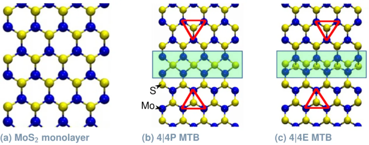
3 One-Dimensional Metallic States in MoS2Mirror-Twin Boundaries 37 3.1 Crystal structure and formation of mirror-twin boundaries . . . 37
3.2 Scanning tunneling microscopy and spectroscopy . . . 38
3.3 Electronic properties of mirror-twin boundaries . . . 40
4 Theoretical Models for 1D States in MoS2Mirror-Twin Boundaries 43 4.1 Non-interacting electrons in a box . . . 43
4.2 Charge-density-wave model . . . 46
4.3 Luttinger liquid in a box . . . 50
4.3.1 TLL model with box-like boundary conditions . . . 50
4.3.2 Charging energy . . . 54
4.3.3 Evaluation of the local density of states . . . 55
4.3.4 Comparison of the TLL model with the STS signal . . . 61
4.3.5 Analysis of longer MTBs . . . 63
4.4 Discussion of the Luttinger-liquid interpretation . . . 66
4.4.1 Tunneling to the substrate . . . 66
4.4.2 Spin-orbit coupling . . . 67
4.4.3 Phonon excitations and life-time of the states . . . 67
4.4.4 Spin backscattering . . . 68
5 Conclusions 71
7.2.3 Langevin equation II: decoupling of modes and buildup of equilibrium
correlations . . . 96
8 Fluctuating Hydrodynamics 101 8.1 The fluctuating diffusion equation . . . 101
8.1.1 Heuristic derivation of hydrodynamic equations . . . 101
8.1.2 Macroscopic state coordinates of hydrodynamics . . . 103
8.1.3 Entropy of hydrodynamic modes . . . 104
8.1.4 Hydrodynamic fluctuations . . . 105
8.2 Hydrodynamic long-time tails . . . 108
8.2.1 Relaxation of hydrodynamic modes on average . . . 108
8.2.2 Finite-sized systems: the diffusion time . . . 109
8.2.3 Relaxation of hydrodynamic fluctuations . . . 110
9 Hydrodynamic Bounds to the Entropy Production for a Quasi-Static Quench 115 9.1 Motivation: adiabatic state preparation . . . 115
9.2 Temperature quench and entropy production for a Brownian particle . . . 117
9.3 Entropy production of hydrodynamic modes after a quench . . . 121
10 The Fluctuating Boltzmann Equation 129 10.1 Prerequisites . . . 129
10.2 The standard Boltzmann equation . . . 131
10.3 Collision noise . . . 136
10.4 Boltzmann long-time tails . . . 141
10.5 Derivation of fluctuating hydrodynamic equations . . . 144
11 The Fluctuating Relaxation-Time Approximation 149 11.1 Derivation of noise correlations . . . 149
11.1.1 Linear relaxation-time approximation . . . 150
11.1.2 Nonlinear relaxation-time approximation . . . 151
11.2 Numerical solution of fluctuating flux-conserving equations . . . 153
11.2.1 Numerical stability . . . 154
11.2.2 Numerical integration of stochastic equations . . . 157
11.3 Numerical evidence of long-time tails . . . 160
11.3.1 Objective . . . 160
11.3.2 General conditions . . . 160
11.3.3 Detailed program flow . . . 162
11.3.4 Analytic prediction . . . 163
11.3.5 Numerical results . . . 164
12 Outlook 171 12.1 Long-time tails after a Fermi-liquid quench . . . 171
12.2 Long-distance tails in a current-carrying wire . . . 173
Contents
A Supplement to Part I 175
A.1 Mean-field theory of the CDW transition . . . 175 A.2 Local density of states via Green’s function method (Lehmann representation) 178 A.3 Evaluation of the LDOS of the TLL model . . . 182
B Supplement to Part II 187
B.1 The Fokker-Planck equation derived from the Langevin equation . . . 187 B.2 Local entropy production and entropy fluxes . . . 188 B.3 Separating rates of entropy production and entropy flux using the multivariate
Fokker-Planck equation . . . 188 B.4 Collision integral: Symmetry and sum rules . . . 189 B.5 Neumann stability analysis of the streaming term: comparison of different dis-
cretization schemes . . . 191
Bibliography 204
Acknowledgments 205
Erklärung und Angabe der Teilpublikationen 207
Preface
The purpose of this preface is to briefly outline the scope of the present thesis and to show how its various subjects may be linked by the concept of scale invariance. We touch upon several concepts here, but introduce them carefully in the main text to the extent that they are needed.
One of the remarkable phenomena observed in condensed-matter or many-particle systems is the emergence of scale invariance [1]. A scale invariant state of matter may be detected by considering the correlations of fluctuations in space and time. Correlation functions measure how strongly the fluctuations at a given point in space and time affect the fluctuations at a distance or at a later time. In many-particle systems, correlations are often expected to decay exponentially fast on short microscopic scales in space and time. In a fluid, typical scales are given by the time elapsing between the collisions of the particles or the mean-free path, respectively. For larger distances or longer times the fluctuations are essentially uncorrelated.
In more interesting situations, the correlations are long-ranged and their decay follows a power- law. Here, characteristic scales are absent. Rescaling of time or space coordinates is equivalent to multiplying the correlation function with a scale factor, i. e. the correlation function is a homogeneous function of space and time coordinates [2]. Owing to this property, we recognize a scale invariant state. We want to highlight three examples of emergent scale invariance:
• The paradigmatic example of scale invariance is critical points of continuous phase transi- tions. According to Landau’s theory of phase transitions the free energy can be expanded in terms of an order parameter φclose to the transition [2].1 The scenario of a second- order phase transition is described by the free energy F[φ] =Rx[rφ2+c2(∂xφ)2+uφ4] with u >0. F[φ] is minimized by hφi= 0 in the disordered phase for r >0 and by hφi=p−r/2u6= 0 in the ordered or symmetry broken phase forr <0. The continuous transition occurs at the critical point r= 0. When the critical point is approached from the disordered side of the transition, the order parameter still vanishes on average, but its fluctuations are enhanced. Within the Gaussian approximation u = 0, the fluctuations of the order parameter decay as
hφ(x)φ(x0)i ∝ 1
|x−x0|d−2+η exp −|x−x0| ξcorr.
!
, (0.1)
in d dimensions [2–4]. As the correlation length diverges as ξcorr. ∝r−ν for r →0, the correlations follow a power-law directly at the critical point. The divergence of the correlation length is driven by the softening of theφ(q= 0) Fourier mode. The values of the critical exponents, η = 0 and ν = 1/2, are predicted wrongly when the fluctuations loose their Gaussian character, e. g. in low dimensions d < 4. The true values are less universal than Landau’s theory suggests. Still, critical systems that fall into a certain universality class share the same exponents. Apart from this refinement, the power laws at and in the approach of critical points remain.
• Fermions in one dimensions loose their identities as single particles that are merely dressed with particle-hole excitations. Instead, they form collective density excitations. The resulting long-ranged correlations of the original fermions are reflected in the power-law
1We restrict ourselves to classical criticality with scalar order parameters, e. g. the Ising ferromagnet.
temperature at a scale ∝ vF/T which diverges for T → 0 [6]. At T = 0, the fermion system can be viewed as exactly at a critical point. More specifically, the fermions tend to order in a density-wave pattern, but the order is suppressed by strong quantum fluctuations [5]. Similarly to critical exponents, the values of α and β change when interactions are included. They are non-universal and depend on the actual interaction strength.2
• Scale invariance is not only restricted to isolated points in phase diagrams where the temperature or other parameters have to be fine tuned to a critical value. Besides critical points, an ubiquitous source of scale invariance is conservation laws. In the ultimate long- wavelength and low-frequency limit, the transport of conserved quantities is described by the equations of fluctuating hydrodynamics [7]. In the simplest case, we think of a single conserved quantity Rxρ(x) and its densityρ(x), governed by a fluctuating diffusion equation ∂tρ −D∂x2ρ = ∂x ·ζ. Here, D is the diffusion constant. The correlations of the fluctuating current ζ are determined by a fluctuation-dissipation relation. The equilibrium correlations of the conserved density in ddimensions,
hδρ(x, t)δρ(x0, t0)i ∝ 1
|t−t0|d/2exp −|x−x0|2 4D|t−t0|
!
, (0.3)
exhibit a so-called hydrodynamic long-time tail ∝ |t−t0|−d/2 for long time intervals.
Similar to classical criticality, the source of the long-ranged temporal correlations is a soft q = 0 Fourier mode: As the total quantity ρ(q = 0) = Rxρ(x) is conserved, the correlations of Fourier modes decay arbitrarily slowly for q →0.
The present thesis covers two subjects which are discussed largely independently of each other.
Still, they have in common that they are more or less closely related to the scale invariant phases mentioned above. The following aspects are addressed:
• We mentioned that the power-law correlations related to criticality and the ones in low dimensions are cutoff at a length scale essentially set by temperature or some other control parameter. The system size introduces an further length scale L. As a consequence, the spectrum of the fluctuations exhibits a gap of size ∝ 1/L. The softening of any mode stops at this scale. The related power-laws eventually turn into exponentials at scales comparable withL. Strictly speaking, critical behavior – and scale invariance in general – is only possible in the thermodynamic limit of infinite system size, i. e. 1/L→0. However, this fact is not particularly relevant for macroscopic systems.
In Part I of the thesis, we deal with the opposite extreme case, a one-dimensional metal of small finite length. Such systems were recently realized as mirror-twin bound- aries (MTBs) of MoS2 monolayer crystals [8, 9]. These nm-sized line defects host one- dimensional metallic states which are well-isolated from the surrounding bulk crystal.
2Additionally, for spinful fermions, the Green’s function factorizes into contributions of the charge and spin sector. The exponents are replaced asα→(αc+αs)/2,β→(βc+βs)/2.
Preface
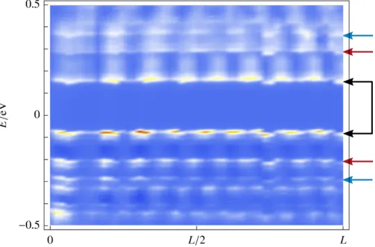
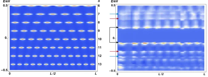
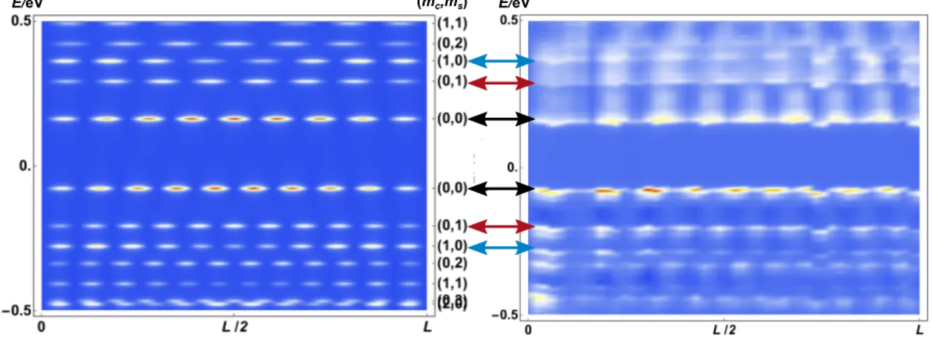
Due to the short length of the MTBs the energy levels are separated by gaps∝1/L. The separation is large enough that isolated levels are resolved in scanning tunneling spec- troscopy (STS) at low temperatures. Away from the thermodynamic limit, the power-law suppression of the density of states related to (0.2) is hard to detect. Instead, the distri- bution of energy levels in the finite-size spectrum is more informative. We calculate the local density of states of a one-dimensional metallic wire of finite length. Comparison of the theoretical spectra of three different models with the STS data allows us to identify the precise nature of the one-dimensional states hosted by MTBs.
• The correlation functions (0.3) characterize fluctuations of thermodynamic equilibrium states. These states are completely defined by the total amount of the conserved quanti- ties of the system, e. g. the total energy. When a system is prepared in a non-equilibrium state, our generic expectation is that the initial correlations will relax to their equilibrium form.
Part II dwells on the formation of hydrodynamic equilibrium correlations (0.3). The long- ranged equilibrium correlations build up only slowly, hampered by the diffusive transport of the conserved quantities. As a consequence, long-time tailshδρ2(x, t)i − hδρ2(x, t)ieq ∝ t−d/2 also emerge in the approach of the equilibrium state as a function of the absolute time t. A microscopic theory has to reproduce the algebraic buildup of fluctuations in the hydrodynamic regime. The Boltzmann theory is a first step in this direction. It provides an equation of motion for a general momentum distribution function of particles fk(x, t) which can also assume a non-equilibrium form. The Boltzmann equation in its standard textbook form [3, 10, 11] neglects correlations and, therefore, does not comprise the scale-invariant stage of the relaxation. However, close to equilibrium the missing piece of information is restored by a fluctuation-dissipation relation, similar to the equations of fluctuating hydrodynamics. Here, we derive a simplified version of the fluctuating Boltzmann theory: a fluctuating relaxation-time approximation. We show how it can be solved numerically and demonstrate the consistency with fluctuating hydrodynamics.
I
Luttinger-Liquid in a Box:
The Spectral Signature of Spin-Charge Separation
in MoS 2 Mirror-Twin Boundaries
1
Chapter 1Introduction I
A beginner’s course on quantum mechanics often starts by discussing particles in one dimen- sion (1D). One of the first problems to be solved is a particle confined to a 1D box of given length. At first glance, this seems to be a rather artificial scenario, intended only for a smooth introduction. One might think that the 1D case is trivial from a theoretical point of view and, more importantly, irrelevant in a three-dimensional world. The study of1D metals leads to a different conclusion: The interacting electron gas in 1D metals is predicted to behave very dif- ferently from electrons in ordinary, higher dimensional metals, which is already an interesting aspect from theory side. Moreover, the scientific interest in 1D metals is significantly increased by the fact that they can actually be produced and investigated in the lab.
1D metals and ordinary higher-dimensional metals are distinguished by the role of interac- tions. In ordinary metals electrons, behave essentially like free fermions despite the fact that they strongly interact. This remarkable fact is explained by Fermi-liquid theory [12, 13]: The low-energy excitations of the interacting system are long-lived fermionic quasiparticles. The quasiparticle states are in a one-to-one correspondence to the states of free fermions. There- fore, interactions do not have much impact. Interacting fermions in 1D behave differently. It turns out that no stable quasiparticles exist in 1D which invalidates the Fermi-liquid concept.
Instead, the single-particle excitations fractionalize into spin and charge degrees of freedom.
The elementary excitations are no longer fermionic quasiparticles. They are replaced by non- interacting spin- and charge-density waves with bosonic statistics. This many-particle state is calledTomonaga-Luttinger liquid (TLL). Similar to a Fermi liquid, the TLL is characterized by a small number of parameters: the velocities of spin- and charge-density wavesuc,us and two further Luttinger-liquid parameters (LLPs) Kc, Ks which encode the interaction strength of the of electron system. The fact that spin and charge appear as independent entities is referred to asspin-charge separation. It was first realized by Tomonaga [14] that fermions in 1D can be described in terms of bosonic degrees of freedom. Later, Luttinger [15] came up with a model of interacting fermions in 1D and showed that the model can be solved exactly. Haldane [16]
recognized that the TLL model is the effective low-energy theory of the 1D interacting electron gas. The exact solution of this model shows that the low-energy excitations are bosonic density waves and the Fermi liquid is replaced by the Luttinger liquid in 1D. Still, one could suspect that solving a 1D problem is a purely academic exercise. Luttinger himself regarded the 1D model as “unrealistic” [15].
Meanwhile there are quite a few examples of 1D metals which could be realized and Luttinger- liquid behavior was observed. Prominent examples are anisotropic crystals which conduct electrons primarly along one crystal direction (quasi 1D materials), e. g. purple bronze [17, 18]
or Bechgaard salts [19, 20], carbon nanotubes [21, 22], the edge channels in quantum Hall systems [23–26], semiconductor nanowires (fabricated by cleaved edge overgrowth) [27, 28], or self-assembled wires of metallic atoms on semiconductor surfaces [29]. More recently, a further
Liuet al. [34] studied a dense network of MTBs in MoSe2 with scanning tunneling microscopy (STM) and spectroscopy (STS). They observed a standing-wave pattern in the STM signal with approximately linear relation between wavelength and energy. The authors explained the dispersing behavior by the confinement of electrons to MTBs of finite length. Following their argument, the result can basically be understood with a model of particles in a 1D box. Barja et al. [35] came to a different conclusion. They performed similar measurements on MTBs in MoSe2 and found a pronounced gap in the energy spectrum at the Fermi energy, accompanied by a periodic modulation of the electron density close to an integer multiple of the lattice constant. They attributed their findings to a Peierls instability. An instability of this type is induced by electron-phonon coupling and leads to a gapped state with broken translation sym- metry. The symmetry-broken ground state is characterized by a macroscopic charge-density wave (CDW) in real space. The explanation of the standing-wave pattern as a result of ele- mentary quantization was rejected. In general, a CDW state is not necessarily commensurate with the underlying lattice as reported there. Maet al. [36] extended the STM measurements to a broader temperature range. They detected CDW transitions atT = 235 K andT = 205 K related to incommensurate and commensurate CDW states, respectively. Furthermore, they studied the dispersion of the 1D states above the CDW transitions at T = 300 K by means of angle-resolved photoemission spectroscopy (ARPES). In order to predict the ARPES signal a refined 1D model was used which is valid also at high energies and converges to the TLL model at low-energies. The theoretical modeling allowed the authors to identify split bands of spin and charge excitations in the ARPES signal. They argued that the observed spin-charge separation proves the 1D nature of the electronic states even at high energies.
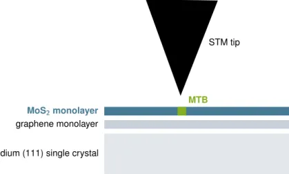
The results of the above-mentioned DFT calculations suggest that MTBs in the related com- pound MoS2 also represent 1D metals. The questions arises what kind of 1D state is realized in MTBs of MoS2. We pursued this question within the framework of a collaboration between experiment and theory [9]. The 1D states localized at the MTBs were investigated by STM and STS measurements. STS was used as a tool for recording the local density of states (LDOS).
The LDOS is a very informative quantity which can be seen as the fingerprint of the 1D system.
We contributed the theoretical calculation of the LDOS as predicted by different models. The comparison between the theoretical LDOS and the STS signal provides strong evidence that the 1D state is a TLL. In the present work, we explain how this conclusion was drawn. We discuss three possible scenarios for the 1D states:
• non-interacting electrons,
• a Peierls-type CDW, and
• a TLL.
For each scenario, we present the calculation of the LDOS and discuss the agreement between the predicted LDOS and the STS data.
Structure Ch. 2 provides an introduction to the peculiarities of the 1D electron gas. We start by reviewing the quasiparticle concept of Fermi-liquid theory and its breakdown in 1D.
Subsequently, we present two collective phenomena which occur in 1D metals: First, we discuss the possibility of a symmetry-broken CDW state as a result of electron-phonon coupling. Here, we analyze the CDW transition on the mean-field level. We then turn to the phenomenon of spin-charge separation. To this end, we introduce the low-energy model of the 1D metal, the TLL model, and show how it can be solved exactly using the bosonization technique. The ele- mentary excitations are found to be independent spin- and charge-density waves. We include a derivation of the so-called bosonization identity which relates fermionic and bosonic degrees of freedom. The identity is an important tool in the calculation of the LDOS of the TLL model.
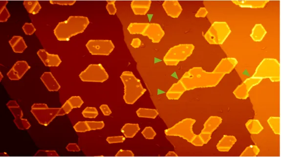
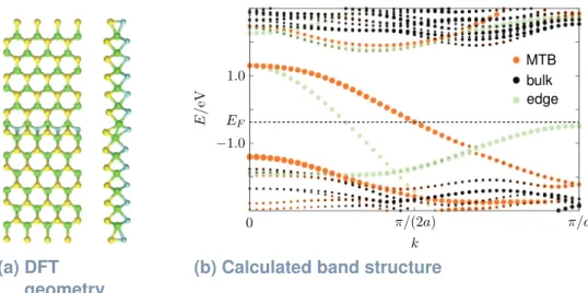
In Ch. 3, we turn to the experimental platform, the MTBs in MoS2. We briefly discuss the experimental conditions, the preparation of monolayer MoS2, and the formation of MTBs. We continue to explain the working principle of STM and STS and relate the LDOS of the sample to the tunnel current in an STM measurement. Finally, we summarize the electronic properties of the MTBs as known from DFT calculations and STS measurements.
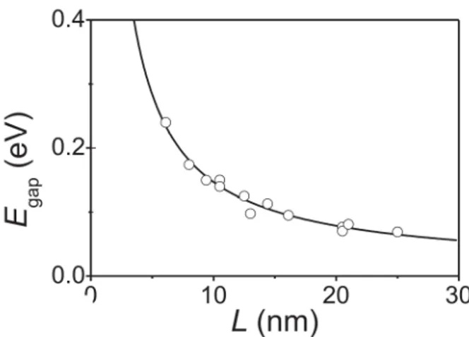
The main chapter Ch. 4 contrasts the STM signal of a short MTB of length L = 6 nm with the theoretical LDOS of three models: non-interacting electrons in a box, a CDW model, and a TLL model. We proceed in the following way: We write down the respective model for a finite geometry of lengthL. For the non-interacting and the CDW model, we obtain the LDOS directly in terms of the energy spectrum and the wave functions. In order to calculate the LDOS of the TLL model, we use the Green’s function method and employ the bosonization identity. For each model, we discuss the similarities and discrepancies between the calculated LDOS and the measured LDOS. Finally, we find that the TLL model describes the experimen- tal findings best. We will interpret the doubling of energy levels in the measured LDOS as a signature of spin-charge separation. After the discussion of the short MTB, we consider longer MTBs. Here, we argue that the Fourier transform of the LDOS is better suited for detecting a splitting of the dispersion. We also use the Fourier transform to estimate the value ofKc. We conclude the chapter by discussing possible objections that could be raised against our TLL interpretation.
Ch. 5 summarizes our conclusions about the nature of the 1D states in MoS2 MTBs.
2
Chapter 2Collective Phenomena in One-Dimensional Metals
In previous studies of MTBs in MoSe2, two different types of 1D collective states were re- ported: a CDW and a Luttinger liquid. In the present chapter, we discuss the theoretical concepts which are needed to describe such 1D states from a general perspective. Through- out the chapter, we consider periodic boundary conditions. In Sec. 2.1, we start by reviewing the quasiparticle concept of Fermi-liquid theory which describes the properties of ordinary metals. With this background, we show that the quasiparticle concept breaks down in 1D, indicating that 1D metals deserve a special treatment. In the following sections, we deal with the collective states of 1D metals: In Sec. 2.2, we introduce the CDW state using a minimal model of a fermionic chain. We continue to develop the BCS-type mean-field theory of the CDW transition which relies on an attractive interaction channel. Finally, we explain how the attractive interaction is mediated by optical phonons and point out the relation to the Peierls structural instability of the underlying lattice. The CDW order breaks translation symmetry. In Sec. 2.3, we turn to the generic, translation symmetric many-particle state of 1D metals: the Luttinger liquid. We set up the TLL model which describes the low-energy excitations of the 1D metal and show that the elementary excitations are independent spin- and charge-density waves using the bosonization technique. We conclude by deriving the bosonization identity which provides the relation between fermionic and bosonic operators.
2.1 What is a one-dimensional metal and why is it different?
2.1.1 Definition of a 1D metal
In classical mechanics, the usual way to confine the motion of particles to one-dimension is to apply suitable forces perpendicular to the desired one-dimensional trajectory. Such forces appear in the Lagrange equations of first kind. In a more realistic modeling the restoring force is generated by some steep potential barrier. Already small deviation from the one-dimensional trajectory are charged with a large potential energy. Only particles with large kinetic energy can move significantly in the perpendicular direction, which happens in an oscillatory way.
Low-energy particles follow almost perfectly the one-dimensional channel with vanishing per- pendicular oscillations.
For a quantum mechanical system, one has to argue differently, see e. g. Refs. [37, 38]: Here, we consider the wave functions of the particles, 2m1 (−∂2x−∂y2−∂z2)ψ(x, y, z) =E ψ(x, y, z). For an infinite wire with cross-section w×w, the eigenvalues are Eny,nz(kx) = 2mk2x +2m1 πw22 (n2y+n2z), where kx is the momentum of the particle moving along the wire and nx, ny ∈N label the standing-wave states which extent in the perpendicular directions. In a generic situation, many standing-wave bands cross the Fermi energy EF at a multitude of Fermi points. As a
in Ch. 3. Further examples of 1D metals created by gapping out the transverse degrees of freedom are heterostructures or carbon nanotubes, see Ch. 1. A different mechanism for the creation of 1D metals is present in highly anisotropic materials which can be described by a tight-binding Hamiltonian [39, 40]. Here, many 1D wires are realized in the direction of the dominant hopping amplitudetx. The coupling to neighboring wiresty, tz can be regarded as a small perturbation.
2.1.2 Fermi-liquid theory and its breakdown in 1D
The properties of ordinary high-dimensional metals are qualitatively well-described, assuming that the electrons form an ideal Fermi gas. At the same time, the Coulomb interaction between the electrons is strong and far from being a small perturbation compared to their kinetic energy.
This seeming contradiction is resolved by Landau’s Fermi-liquid theory which is based on the principle of adiabaticity together with Pauli’s exclusion principle for fermions [12]. Our brief discussion of Fermi-liquid theory and its breakdown is based on the textbooks by Coleman [4]
and Bruus and Flensberg [37].
Fermi-liquid theory states that interacting fermions essentially behave like non-interacting fermions: At low energies, the elementary excitations of the interacting fermion system are fermionic quasiparticles which are labeled by the same quantum numbers, momentum and spin (k, σ), but their mass is renormalized and they acquire a finite life-time.2 The life-time diverges at the Fermi surface and, therefore, low-energy excitations of the Fermi liquid are well-described as quasiparticles states. In the following, we briefly summarize Landau’s argu- ment: Consider the time-dependent many-body HamiltonianH(t≥0) =H0+ (1−e−λt)Hint, where we switch on electron-electron interactions at t = 0 at a rate λ.The principle of adia- baticity states that if the interaction Hint is switched on slowly enough the eigenstates of the non-interacting Hamiltonian at t= 0 evolve to the eigenstates of the interacting Hamiltonian att=∞,|ψinti =U(∞,0)|ψ0i, with the time-evolution operator U(∞,0). From this notion we can infer that the non-interacting ground state|ψ0GSi is equivalent to the ground state of the interacting system.3 The filled Fermi sea is the ground state of the Fermi liquid. The relation between the excited states of the non-interacting and the interaction system is estab- lished through the fact that an electron with energyk close to the Fermi sea is a long-lived object since the phase space of the decay process is restricted by Pauli’s exclusion principle.
To rationalize the argument one considers the decay of an electron |pki on top of the Fermi sea to a state closer to the Fermi surface|pk+qi. Due to energy (and momentum) conservation a particle-hole pair|pk0−qhk0i has to be created. According to Fermi’s Golden Rule the decay
1We assume inversion symmetry.
2There are residual interactions, but they preserve the (infinite) number of conservation laws.
3The statement is true unless no level crossing occurs which would be related to spontaneous symmetry break- ing.
2.1 What is a one-dimensional metal and why is it different?
rate of the process|pki → |pk+qpk0−qhk0i can be estimated by Γk = 2π
~
Z d3k0 (2π)3
Z d3q
(2π)3|Vq|2δ(k+k0 −k+q−k0−q)fk01−fk+q 1−fk0−q
. (2.1) Vq denotes the momentum conserving electron-electron interaction. The factors (1−fk+q), (1−fk0−q) express the Pauli principle: The particles can only scatter to an empty state. For clarity, we neglected the spin quantum number. AtT = 0, we havefp=θ(−p) and the decay rate for a particle above the Fermi seak>0 can be estimated as
Γk ∼ |V|2ρ3F Z0
−∞
d0
∞
Z
0
d00θ(k+0−00) = |V|2ρ3F2k
2 . (2.2)
The Pauli principle enforces the initial electron states to decay to a final state within a shell of widthk above the Fermi level. Due to energy conservation an electron-hole pair is created in the decay process, where the hole is created in a shellkbelow the Fermi energy. Therefore, the phase space of the decay is restricted by the factor∼2k.4 Interpreted in terms of a single- particle wave function, ψ(r, t) ∼ eik·reikte−Γkt, (2.2) states that the wave function oscillates many times before it is damped out, i. e. the excited particle can propagate for a long time before it decays due to the interactions. Thus, it is possible to choose the switching rateλ in the window Γk ∼2k λ k, slow enough that ground state and excited states do not mix and fast enough that excited states do not decay during the switching process. Therefore, the low-energy states of the interacting Fermi liquid are again described by fermionic particles, the so-called Fermi-liquid quasiparticles, which are in a one-to-one correspondence with the physical electrons. They are labeled by the same quantum numbers α = (k, σ). The relation between quasiparticles and physical electrons is also reflected in the finite overlap of the corresponding operators. The quasiparticle operator has the expansion
d†α = Uλ†(∞,0)c†αUλ(∞,0) λ→0
= √
Zαc†α+X
βγδ
Aαβγδc†βc†γcδ+O(c†,(c†c)2). (2.3) The quasiparticle weight 0< Zα ≤1 indicates that the one-to-one relation holds. Still, it is not a perfect identity: The quasiparticle is not just an electron, but an electron surrounded by a cloud of particle-hole excitations. The heuristic argument outlined above is also confirmed by diagrammatic perturbation theory of the fermionic Green’s function. Here, the effective mass, decay rate, and quasiparticle weight are derived from the expression of the (one-particle irreducible) self-energy. Close to the pole atω=∗k, the (retarded) Green’s function is modified as
GR,0k = 1
ω−k+ iδ → GRk = 1
ω−k−Σk(ω)
ω≈∗k
= Zk
ω−∗k−iΓk. (2.4) The δpeak of the non-interacting electrons is replaced by
A0k(ω) = δ(ω−k) → Ak(ω) = ZkδΓk(ω−∗k) +Ainc.k (ω). (2.5) Compared to the spectral function of free particlesA0k(ω), the quasiparticle peak is broadened by the finite decay rate Γk and its weight is reduced toZk <1. The remaining fraction of the spectral weight, 1−Zkis absorbed by so-called incoherent excitations. Close to the Fermi sur- face the quasiparticle peak becomes very sharpand is clearly distinguished from the incoherent background, indicating well-defined quasiparticles.
4For finite temperaturesT k, (2.2) gives Γk∼T2 which is relevant to transport in a Fermi liquid at finite temperatures.
as a prefactor,
Γk ∝ X
k0,p,p0=±kF
δ(k+k0−p−p0) =? ∞. (2.6) Indeed, it can be shown that Γk ∼ k, indicating that the decay rate can never be regarded as small ind= 1. Interactions are always strong perturbations. Stable quasiparticles do not exist, even close to the Fermi surface.
In order to gain further insight, we consider the polarization operator or electronic susceptibility inddimensions,
Πq(ω) = gS
Z ddk (2π)d
f(k+q)−f(k)
ω−k+q+k+ i0+ . (2.7)
The polarization operator describes how the electron system reacts to charges and is also a central building block of the self-energy diagrams in diagrammatic perturbation theory. The factorgS = 2 results from the spin-degeneracy. In the following, we focus on the static suscep- tibility Πq(ω= 0)≡Πq. For small momenta |q| kF, the polarization operator evaluates to a constant, yielding the density of states at the Fermi level Πq=ρF, in arbitrary dimensions.
Its constant value leads to static screening of the Coulomb potential. For momenta|q| ≈2kF, the polarization operator shows an interesting behavior, which has profound physical conse- quences. Ford= 3,2 the polarization operator has a logarithmic singularity in its derivatives.
This weak singularity is called Kohn anomaly and adds slowly decaying 2kF oscillations to the effective interaction potential, ∼ cos(2krFdr+δ), known as Friedel oscillations [41, 42].5 In d= 1, the polarization operator itself diverges logarithmically at |q|= 2kF. The reason for the di- vergence lies in the simple topology of the Fermi surface in 1D, consisting only of two isolated points±kF which are exactly connected by a q =±2kF scattering process. This situation is referred to as perfect nesting.6 The singularity has important consequences:
• As the polarization operator appears as central building block in the perturbation theory of the Fermi liquid, the logarithmic divergence enters the expansion of the self-energy and invalidates the quasiparticle concept: The quasiparticle weight, derived from the self-energy, vanishes, Zk= 0.
• As the polarization operator describes the response of the electrons to external charges, the divergence of the polarization operator signals an instability of the electron system towards spatial modulations of the charge with period 2k2π
F = kπ
F.7
The analysis of the polarization operator atT = 0 suggests that the 1D interacting electron gas forms a density wave with spontaneously broken translation symmetry and its ground state is characterized by the corresponding order parameter, at least at sufficiently low temperatures.
According to this line of reasoning, Fermi-liquid theory is replaced by a theory of the density- wave state and its fluctuations around the new ground state. We discuss the mean-field theory
5δ is a phase shift.
6In higher dimensions only small patches of a spherical Fermi surface are connected by 2kF and the divergence is removed.
7The nature of the density wave also depends on the sign of the 2kF amplitude, see Sec. 2.2.
2.2 Charge-density-wave transition
of the density wave in Sec. 2.2.
On the other hand, it is well-known that 1D systems of any kind cannot develop long-range order at any finite temperature by breaking a continuous symmetry according to the Mermin- Wagner theorem. Strong fluctuations of the order parameter destroy the ordered phase [43].
Thus, a 1D electron gas has a strong tendency towards density-wave order, but cannot or- der. In summary, a strictly one-dimensional metal is a highly correlated electron system, but neither is a Fermi liquid with well-defined quasiparticles nor orders to a densitywave. Fortu- nately, it turns out that the problem of interacting low-energy fermions in 1D can be mapped to non-interacting bosons at low energies and can be solved exactly. The elementary bosonic excitations of the 1D electron gas are identified as collective spin and charge excitations. In this way, it can be shown that the electrons fractionalize into spin and charge degrees of freedom.
As we mentioned in Ch. 1, the theory of the low-energy excitations is provided by Tomonaga- Luttinger-liquid (TLL) theory and the corresponding many-particle state is called a Luttinger liquid. Similarly to a Fermi liquid, the Luttinger liquid is characterized by a small number of parameters. In Sec. 2.3, we choose the constructive bosonization approach to introduce TLL theory.
2.2 Charge-density-wave transition
2.2.1 Minimal model: fermions on a lattice with nearest-neighbor repulsion Let us consider a model ofNF spinless fermions on aN-site chain with lattice constant a. As a special ingredient, we add a term ofnearest-neighbor repulsion,
H = −J
N
X
j=1
c†j+1cj+c†jcj+1
+V
N
X
j=1
ρjρj+1, (2.8)
with hoppingJ >0 and nearest-neighbor repulsionV >0. ρj =c†jcj is the occupation number operator of site j. We assume periodic boundary conditions, i. e. the fermions hop on a ring with c†N+1 = c†1, cN+1 = c1. In order to determine the T = 0 ground state of the fermionic chain, we have to find the configuration{ρi} which minimizes the energyh{ρi}|H|{ρi}ifor a fixed number of lattice sites N and fermions NF. For generalN and NF, the solution is not unique, i. e. the ground-state manifold is degenerate. The ground state configuration avoids nearest-neighbor relations since they come with an extra interaction energy V for each pair of adjacent fermions. A configuration with minimal number of nearest-neighbor relations is in the ground state manifold. Here, we want to consider a chain with even number of sites at half-filling,N = 2NF. In this case, the ground state manifold is doubly-degenerate. Empty and occupied sites alternate along the chain with periodicity 2aand without any nearest-neighbor relations for both of the two possible ground state configurations. Anticipating that an oc- cupied site is related to an accumulation of charge, we may call this alternating pattern a charge-density wave (CDW).
In the following, we analyze the requirements for a CDW. Translating the hopping Hamiltonian to momentum space,
cj = 1
√ N
X
k
eikajck, c†j = 1
√ N
X
k
e−ikajc†k, (2.9) leads to the dispersionk=−2Jcos(ka) with the Brillouin zone −πa < k≤ πa. At half-filling, the cos band is occupied up to the Fermi momentumkF = 2aπ. The full Hamiltonian reads as
H = X
k
kc†kck+ 1 N
X
k,k0,q
Vqc†k+qckc†k0−qck0, (2.10)
In order to limit the modifications, we still restrict the discussion to an even number of sites at half-filling,N =N++N−, and an unpolarized ground state,N+=N−. Now, half-filling refers to one particle per site. For U V, the nearest-neighbor repulsion ∼ V Pσσ0,jρj,σρj+1,σ0 = P
σσ0,qVqρq,σρ−q,σ0 favors a CDW configuration. In this state, the charged sites are occupied by two fermions of different species σ = ±. Charged and empty sites again alternate with the wave vector 2kF. In the opposite limit of U V, the on-site repulsion enforces an occupation of one fermion per site and destroys the charge-density wave. We recover the standard Hubbard model [44]. The ground state configuration is known to be antiferromagnetic.
We can regard the antiferromagnetic configuration as two spin-polarized waves which are shifted by one site to satisfy the on-site repulsion and realize aspin-density wave. Indeed, the Hubbard- U only affects the interaction between densities of opposite spin,Pq(U +Vq)ρq,+ρ−q,−, while interaction between densities of same spins,PqVq(ρq,+ρ−q,++ρq,−ρ−q,−), remain unchanged.
The antiferromagnetic state also minimizes the interaction energy of the latter term since the spin-polarized density waves remain.8 In the following, we only cover the CDW case, i. e. a situations with net interactionV2kF <0.
2.2.2 Continuum model and mean-field analysis
We will show that an attractive 2kF channel is indeed responsible for an instability towards the CDW ground state. The mean-field analysis presented here is inspired by the BCS theory of superconductivity [4].
We focus on the low-energy sector of the fermionic chain in (2.10). Only states in a narrow re- gion around the Fermi points are relevant,±kF +k, where−Λ≤k≤Λ. The cutoff momentum Λ is a small momentum scale which plays the role of an effective band width. Fermions near
±kF are identified as right- and left-moving particles. We introduce the notationc†−k
F+k ≡c†L,k, c†k
F+k ≡c†R,k for operators creating left- or right-moving particles, respectively. Furthermore, we may linearize the bands of left and right movers asR/L,k≡±kF+k=±vFkwith the Fermi velocityvF =∂kk|k=kF in the low-energy region. Here, we assume symmetric bands. Adding spin degrees of freedom, Pk → Pk,σ, does not affect the form of the final expressions. The density of state is then understood to include both spin species.
The restriction to two isolated bands around the Fermi points implies that the low-energy fermions only interact via theq = 0 and q= 2kF scattering channels. The low-energy Hamil- tonian derived from the lattice Hamiltonian (2.10) reads as
H =
Λ
X
k=−Λ
vFk
−c†L,kcL,k+c†R,kcR,k
+V2kF N
Λ
X
k,k0=−Λ
c†L,kcR,kc†R,k0cL,k0+ V0
NNF2. (2.11) We neglect the global energy shift∝NF2 caused by theq = 0 channel.9 A CDW with periodicity
8We expect a quantum phase transition between the CDW and the AFM phase, for U +V2kF = 0, if the attractive channel vanishes due to large on-site repulsion.
9Note that the total number of fermions is conserved, [H, NF] = 0.