Order and transport in interacting disordered low-dimensional systems

Order and transport in interacting disordered low-dimensional systems

Inaugural-Dissertation zur

Erlangung des Doktorgrades

der Mathematisch-Naturwissenschaftlichen Fakult¨at der Universit¨at zu K¨oln

vorgelegt von

Zoran Ristivojevic

aus Kruˇsevac, Serbien

K¨oln 2009

Berichterstatter: Prof. Dr. Thomas Nattermann

Prof. Dr. Matthias Vojta

Tag der m¨ undlichen Pr¨ ufung: 03. Juli 2009

iii

Contents

Contents iii

1 Introduction 1

1.1 Physical systems . . . . 1

1.2 Interacting electrons in one dimension . . . . 3

1.3 Thin superconducting films . . . . 7

1.4 Outline of the thesis . . . . 9

2 Transport in a Luttinger liquid with dissipation 11 2.1 Introduction . . . . 11

2.2 Model . . . . 13

2.3 Renormalization group analysis . . . . 14

2.4 Transport . . . . 17

2.5 Friedel oscillations . . . . 20

2.6 Conclusions . . . . 21

2.A Conductance from the Fermi golden rule . . . . 21

3 Realization of spin-polarized current in a quantum wire 25 3.1 Introduction . . . . 25

3.2 Model . . . . 28

3.3 Resonant tunneling of spinless electrons . . . . 31

3.4 Weak impurities . . . . 33

3.5 Strong impurities . . . . 35

3.6 Transport . . . . 38

3.7 Conclusions . . . . 40

3.A Bosonization . . . . 40

3.B Bosonized model . . . . 45

4 The effect of randomness in one-dimensional fermionic sys- tems 47 4.1 Introduction . . . . 47

4.2 Model . . . . 49

4.3 Rigidities and ac conductivity . . . . 50

iv Contents

4.4 Fixed points and phases . . . . 51

4.5 Mott-glass phase . . . . 53

4.6 Disscussions and conclusions . . . . 55

5 Vortex configurations in a superconducting film with a mag- netic dot 57 5.1 Introduction . . . . 57

5.2 Model . . . . 59

5.3 Ground states with vortices . . . . 62

5.4 Magnetic field . . . . 64

5.5 Numerical study of ground states with low number of vortices 67 5.6 Discussions and conclusions . . . . 72

5.A Derivation of the model . . . . 73

5.B Calculation of U mv . . . . 77

6 Superconducting film with randomly magnetized dots 79 6.1 Introduction . . . . 79

6.2 Model and its solution . . . . 81

6.3 Discussions and conclusions . . . . 84

6.A Equivalence between random potentials . . . . 86

Bibliography 89

Acknowledgements 97

Abstract 99

Zussamenfassung 101

Erkl¨ arung 103

Curriculum vitae 105

1

Chapter 1

Introduction

In this chapter we introduce two different systems that will be con- sidered in this thesis: one-dimensional interacting electronic systems and thin superconducting films.

1.1 Physical systems

Physical systems are very diverse and can be classified in many ways. They can be macroscopically large or microscopically small regarding their size, they can be solid, liquid or gaseous with respect to their state, and there are many other classifications with respect to some property. While some physical systems are well understood, many of them are not. The main obstacle hindering a thorough understanding is the interaction. For systems that we will investigate in this thesis, it is the electromagnetic interaction that is responsible for non-trivial physical effects. The other three fundamental interactions are irrelevant for our considerations.

We begin with a simple example which demonstrates one aspect of the space dimensionality. The electromagnetic potential Φ(r) produced by the charge density ρ(r) is governed by the Poisson equation [1]

∇ ² Φ(r) = − 4πρ(r). (1.1)

The solution of the previous equation for a single electron placed at the origin depends on the system dimensionality d. It is given by

Φ(r) =

 



− e/ | r | , d = 3, const − 2e log | r | , d = 2, 2πe | r | + const, d = 1.

(1.2)

While the electron charge − e enters the potential in the same way in different

dimensions, the spatial coordinate does not. For the interaction between two

electrons the previous expression gives the usual Coulomb 1/r interaction in

three dimensions, but a logarithmic interaction in two dimensions. We see

that even the simplest interacting system shows significant differences in the

2 Introduction

potential energy behavior. We should be aware that an interacting many body system has quite often an effective interaction that is different from the aforementioned Coulomb interaction. The reason for this are complicated many body interaction processes that occur in reality and which can not be all treated exactly. However, at the end an effective picture emerges as a result of some well suited approximative treatment. For example, it is well known that two electrons of opposite spin and momentum effectively attract each other in superconductors. This occurs due to the presence of phonons that mediate the electron-electron interaction in that particular case.

Apart from interaction, other principles of physics are also involved.

Quantum-mechanical indistinguishability of particles classifies them into fer- mions and bosons, apart from possible exotic particles in some two-dimen- sional systems. At large temperatures quantum mechanics is not important any more, rather laws of classical mechanics apply. There both kinds of parti- cles behave similarly. At low temperatures fermions and bosons behave quite differently, due to the Pauli exclusion principle. It states that two identical fermions can not occupy the same quantum state simultaneously.

In three dimensions, non-interacting fermions at zero temperature fill the available quantum states up to the Fermi level, while non-interacting bosons condense in a macroscopic quantum state all having zero momentum.

This defines the ground state (the state having the lowest possible energy) of non-interacting fermions and bosons. The lowest-lying excitations in the fermionic case occur when a fermion near and below the Fermi level is excited to an empty quantum state above it. In the bosonic case an excitation consists of taking a boson from the rest state, where it has zero momentum, to a moving state.

Effects of interactions in the systems from the previous paragraph are also well understood. Upon switching-on interactions, the Fermi level is still well defined. The low-energy excitations may be described by quasi-particles.

They satisfy Fermi-Dirac statistics and carry the same spin, charge and mo- mentum as the original fermions, but have a renormalized mass. These quasi- particles are nearly free and have a finite lifetime, which is inversely propor- tional to the square of the excitation energy measured relative to the Fermi energy. The theory of interacting fermions in three dimensions is known as Landau’s Fermi liquid theory [2].

While interaction between fermions in three dimensions does not qual- itatively alter the non-interacting picture, for bosons this is not the case.

Weakly interacting bosons become superfluid at low temperatures. Exper-

imentally, a superfluid flows without friction through narrow capillaries at

low temperatures. For ⁴ He atoms it occurs below the lambda line, at satu-

rated vapor pressure below 2.17 K [3]. Theoretically, due to interactions the

1.2 Interacting electrons in one dimension 3

lowest part of the spectrum of quasi-particles, which diagonalize the inter- acting Hamiltonian, becomes linear, which is a necessary condition for the frictionless flow. Excitations of interacting bosons are of collective nature.

The system dimensionality is also very important. Opposite to the three- dimensional case, non-interacting bosons do not condense in one and two space dimensions due to large fluctuations [3, 4]. Quite generally, effects of thermal fluctuations are drastic in two- and less-dimensional systems, pre- venting long-range order in systems with a continuous symmetry [4, 5].

These are just some very well known facts where the interplay between fluctuations, interaction and dimensionality leads to different physical sce- narios. Another very important ingredient is disorder. In solid state physics systems it can be thermal, due to thermal fluctuations, topological, due to topological defects and compositional, due to externally immersed particles into the host system [6]. Effects of disorder are very important, in particular in low-dimensional systems. This will be also shown in this thesis. In the rest of the thesis we will be dealing only with disordered low-dimensional systems, i.e. with one- and two-dimensional interacting systems. More precisely, we focus on systems that are described as if they were effectively low-dimensional. The one-dimensional systems that we consider are inter- acting electrons, while the two-dimensional systems are thin superconducting films.

1.2 Interacting electrons in one dimension

The effects of interactions in one-dimensional fermionic systems are drastic.

Fermi liquid theory breaks down and one does not have low-energy excita- tions that have a single-particle character. Rather, the excitations become collective. Due to their spin and their charge, electrons are described by two kinds of collective excitations, for the charge and for the spin degrees of freedom. These excitations have different velocities, which has also been confirmed experimentally [7]. This phenomenon, that an interacting one- dimensional electron systems has different velocities of collective excitations, is known as spin-charge separation.

In the non-interacting case the Fermi level reduces to two Fermi points,

± k F . Effects of interactions between electrons in one dimension can be

treated using the bosonization technique [8]. There, one diagonalizes a fermi-

onic Hamiltonian by going over to a bosonic one. Some details about the

procedure are presented in appendix 3.A of chapter 3. Loosely speaking,

bosonization translates interacting fermions into free bosons. We should

stress here that bosonization properly covers only the low-energy part of the

4 Introduction

fermionic spectrum, and in the rest of the thesis we should bear this in mind.

In the following we consider only spinless electrons for simplicity. The two parameters that play a role in the bosonic description are the velocity of excitations v and the Luttinger parameter K. The velocity of excitations is the Fermi velocity modified by interaction, while the parameter K controls the interaction. In the non-interacting case we have K = 1, while for re- pulsive (attractive) interactions we have K < 1 (K > 1). Apart from these two parameters, the bosonic Hamiltonian contains also canonically conjugate position and momentum operators of particles.

Within the classical physics, repulsively interacting electrons in one di- mension at zero temperature are equidistantly distributed, where the dis- tance between two electrons is determined by the electron density. However, their quantum-mechanical nature prevents that. The Heisenberg uncertainty relation

∆x∆p ≥ ~

2 (1.3)

requires a completely undetermined momentum for an electron that has a specified position. Oppositely, zero momentum of an electron implies that it is positioned everywhere in space with equal probability. A compromise between these two cases is that both the electron’s position and momentum are fluctuating quantities. This is a quantum-mechanical consequence. To describe particles, one introduces the operator ϕ _i which measures the position of the electron, indexed by i with respect to its classical lattice position.

Going over to the continuum limit, ϕ i translates into the displacement field ϕ(x). The momentum Π(x) is introduced as the canonically conjugated field to ϕ(x) and they satisfy the bosonic commutation relation

[ϕ(x), Π(y)] = i ~ δ(x − y). (1.4)

The two parameters, v and K, and the two fields, ϕ and Π, completely de- scribe the interacting electrons in one-dimension. A new state of matter that arises is called the Luttinger liquid. It is experimentally realized in a number of different systems, which include carbon nanotubes [9, 10], polydiacetylen [11], quantum Hall edges [12], semiconductor cleaved edge quantum wires [13], and in one-dimensional ultra-cold gases [14].

The effects of disorder on Luttinger liquids are also well known. We

distinguish between two kinds of disorder, that are an isolated point impu-

rity and densely spaced many weak impurities that act collectively. While

some interesting effects may occur when impurities are not static [15], in the

following we concentrate only on static impurities.

1.2 Interacting electrons in one dimension 5

Without impurities a Luttinger liquid is perfectly conducting, so we can say that it has metallic properties [8]. We review the influence of impu- rities starting from the non-interacting case K = 1. In the presence of a single impurity the analysis can be done inside the one-body Schr¨odinger equation, from which we simply conclude that an incident wave (electron) is partially transmitted and partially reflected by a potential barrier created by the impurity. This means the non-interacting system remains metallic due to nonzero transmission. The case with many impurities is more complicated.

An electron can coherently backscatter from many impurities and it is not a priori clear whether an electron inserted in the middle of the system can leave it or not. By now it is well established that any disorder in one dimension localizes all electronic states [16, 17], meaning the electron will be localized by disorder. We get an insulating state at zero temperature. Without in- elastic scattering processes, the finite temperature conductivity remains zero.

When inelastic processes are accounted for, like electron-phonon interaction, the situation changes. With the assistance of phonons, electrons may hop between localized states at any non-zero temperature, leading to a small, but non-vanishing conductivity. This form of electron conduction is known as hopping conductivity [18].

When the interaction is switched on, the situation becomes different. A single point impurity of any strength placed into a Luttinger liquid has a very strong effect. For any repulsive interaction it makes the system insulating at zero temperature [19, 20, 21]. Oppositely, for attractive interaction the presence of an impurity is unimportant and the system remains metallic;

this means the phase transition occurs at zero temperature for K = 1. At finite temperature the conductance vanishes with temperature as a power law controlled by the interaction parameter K. In this thesis we will consider a system that consists of a single impurity and in the presence of dissipation.

Qualitatively, the dissipation may be understood as an inelastic scattering process that diminishes the conductance. We will show that in chapter 2.

Another interesting situation occurs when the two barriers, made by two point impurities, are present in a Luttinger liquid. Somewhat surprisingly and opposite to the single impurity case, the system may be metallic for not too strong repulsive interactions. This rather subtle phenomenon is known in quantum mechanics of non-interacting particles as resonance tunneling [22].

A free particle that impinges on the two-barrier potential always tunnels through the potential. In the special case, when its incident wavevector matches the wavevector it would have if the barriers were impenetrable, there is no reflection and the transmission coefficient is one. This is the resonant tunneling phenomenon.

In the interacting case, when the barriers are large in comparison to the

6 Introduction

Fermi energy, the island in between them has a well defined charge. For an electron driven by an external voltage, there are two possible ways to over- come the barriers. One option is direct tunneling through both impurities, and the other is the process of sequential tunneling, where an electron first enters the island from one side and then leaves it at the other. The former process is inhibited by the product of strengths of the barriers, while the latter is inhibited by the strength of one barrier and also by the electrostatic repulsion from other electrons that sit on the island. The electrostatic repul- sion that prevents an electron to enter the island is known as the Coulomb blockade. When the chemical potential on the island is such that adding another electron to the island has no cost in energy, the Coulomb blockade is lifted. In addition, if the interaction is not too strong, the double-barrier is fully transmitting [20] at zero temperature. When the Coulomb blockade is not lifted, the two impurities effectively act as a single one, and the system is insulating at zero temperature.

An external magnetic field tends to split electrons at the Fermi level.

Electrons having different spin projection on the direction of the magnetic field acquire different Fermi momenta. If a double barrier is placed in such a system, an interesting situation may occur. Because electrons of different spin projection have different Fermi momenta, it may happen that just one spin direction resonantly tunnels. This leads to a spin filtering effect. As we know, the effects of interactions are very important in one dimension and they will be examined in chapter 3.

A different kind of disorder is realized when the system contains many impurities that are densely distributed and very weak, so they act collectively.

This kind of disorder is called Gaussian disorder. It is characterized by a single parameter, that is the product of the impurity density and the typical squared single impurity strength [8]. The Gaussian disorder couples to the electron density. It tends to deform the electron displacement field according to its minima, while the electrons classically tend to have the displacement field undistorted. The competition between these two effects, the elastic energy and the disorder, crucially depends on the Luttinger parameter K . For K > 3/2 the elastic term wins and the low-energy properties of the system correspond to the free Luttinger liquid model without disorder. For K < 3/2 the system is disorder dominated and the displacement field is pinned by the disorder. The resulting phase is called the Anderson insulator.

Another kind of ordering in Luttinger liquids occurs when a periodic po-

tential is present in the system. Effectively, the periodic potential may arise

due to umklapp processes [8, 23]. It wants to keep the electron displace-

ment field constant in order to minimize the total energy. The displacement

field “trapped” by the periodic potential is a ground state of the system as

1.3 Thin superconducting films 7

long as the fluctuations of the displacement field, which are measured by K, are small enough. When K increases, the displacement field is “less and less arrested” by the periodic potential, becoming free for sufficiently large K. The low-K phase is known as the Mott insulator for electronic systems.

When both the periodic potential and the Gaussian disorder are present, the situation is complicated since the two insulating phases compete. We will consider this issue in chapter 4.

1.3 Thin superconducting films

Superconductivity was discovered nearly a century ago. The two hallmarks of superconductivity are perfect conductivity and perfect diamagnetism [24].

Inside the phenomenological Ginzburg–Landau theory, one introduces the local superconducting order parameter ψ(r) in order to describe the super- conducting state. The density of superconducting electrons equals n s (r) =

| ψ(r) | ² and is nonzero in the superconducting phase. The correlation func- tion h ψ ^∗ (r)ψ(0) i (where h . . . i denotes an average over the Ginzburg–Landau energy functional) acquires a finite value for | r | → ∞ in three dimensions for temperatures T smaller than the critical temperature T c , which means that there is long-range order for the parameter ψ. For T > T c the corre- lation function decays exponentially and there is short-range order for the parameter ψ.

A strong magnetic field always destroys superconductivity. In type-I su- perconductors this process appears as an abrupt magnetic flux penetration through the whole sample when the external magnetic field exceeds the ther- modynamic critical field. In type-II superconductors, for external magnetic fields between the lower and the upper critical field, magnetic flux penetrates the sample only partially in the form of regularly distributed flux lines. The density of superconducting electrons vanishes inside a flux line, and there normal electrons are present. A flux line, also called a vortex, has a typical spatial extension ξ in the transverse direction. The parameter ξ is called the coherence length and is a characteristic of the superconductor. The magnetic field around a vortex decays over distances beyond the London penetration depth λ L . This is the length scale determined by the electromagnetic re- sponse of the superconductor. A single vortex line has the energy per unit length [24]

ǫ 1 = φ 0

4πλ _L 2

ln λ L

ξ , (1.5)

meaning its energy becomes large for samples long in the direction parallel

8 Introduction

to the vortex (and the external magnetic field). This explains the fact that vortices do not appear due to thermal fluctuations in three-dimensional su- perconductors in zero magnetic field. By φ 0 = hc/(2e) we have denoted a flux quantum.

Thin superconducting films are effectively two-dimensional systems, where the effect of thermal fluctuations is very pronounced. Divergent fluctuations of the phase of the order parameter at low temperatures prevent a true long- range order of the order parameter. Rather, the low-temperature phase shows quasi-long-range order, h ψ(r)ψ(0) i ∼ | r | ^{− η(T )} , where η(T ) ∼ T . The effect of magnitude fluctuations of the order parameter are also very important in two dimensions. We should make a distinction between small fluctuations in the magnitude of ψ, where ψ does not vanish, and large fluctuations, where ψ reaches zero value. The former lead to a slight renormalization of the pa- rameter η(T ) for low temperatures [25], and are not important. The latter play a very important role. Points where ψ( r ) = 0 define vortices. As a difference to the three-dimensional case, here vortices appear due to thermal fluctuations, even in the absence of an external magnetic field. We will show this now.

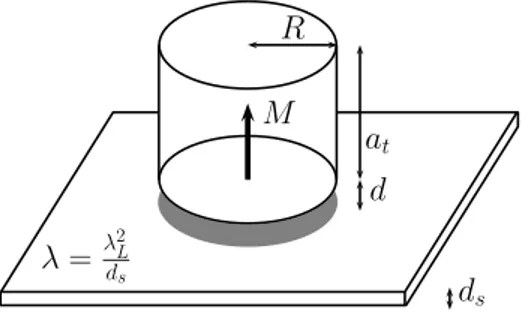
For thin superconducting films it is very important that the magnetic field and the vector potential do not vanish out of the film plane, whereas the order parameter exists only in the film plane. This difference with respect to the three-dimensional case leads to a new effective penetration depth for films, λ = λ ² _L /d s , where d s is the film thickness [25, 26]. This affects the single vortex energy, and also the energy of a vortex-antivortex pair separated by a distance r, which respectively read

U v ≈ ε 0 ln min(λ, L)

ξ , (1.6)

U vv (r) = 2ε 0 ln r

ξ , r < L < λ, (1.7)

where

ε 0 = φ ² ₀

16π ² λ (1.8)

and L is the typical lateral film size. Analyzing the free energy of a single

vortex [27] F = U v − T S, where S = ln(L/ξ) ² we conclude that the two

different possibilities arise. For large system sizes, L > λ, the entropy term

always prevails, meaning any nonzero temperature leads to the spontaneous

appearance of free vortices. This ultimately leads to short-range order of the

order parameter and the film loses its superconductivity. The more inter-

esting case is when L < λ. Then, free vortices are created just above the

1.4 Outline of the thesis 9

critical temperature T 2D = ε 0 /2. We set Boltzmann’s constant to k B = 1 in the following. Below T 2D the system has only bound vortex-antivortex pairs.

They are very important excitations of the amplitude of the order parame- ter not only in thin films, but in a broad class of two-dimensional systems with continuous symmetry. These systems include superfluid films and pla- nar magnets. Using the renormalization group method one can show that the transition temperature becomes T 2D = ε 0 (T 2D )/2, where ε 0 (T 2D ) means that one should use the renormalized value for λ in expression (1.8). This comes from the renormalization of the vortex-antivortex interaction (1.7) due to the presence of other bound vortex-antivortex pairs at low temperatures [25, 28]. Hence, the quasi-long-range order of the order parameter survives at low temperatures T < T 2D , and vortex-antivortex excitations do not destroy this kind of order. The low-temperature phase is superconducting in the sense that it has a nonlinear current-voltage relation of the form V ∼ I ³ at T → T _2D ⁻ . The high-temperature phase, for T > T 2D , behaves like a normal metal and we have V ∼ I [29].

In this thesis we will consider a thin film in the presence of small magnetic dots placed on top of it. Such magnetic nanostructures can be easily cre- ated experimentally and are an interesting tool for probing different physical phenomena [30, 31]. The magnetic substructure creates the inhomogeneous magnetic field in the film and may cause creation and pinning of vortices in the film. It also changes the transport properties and the transition tem- perature of the superconductor. In particular, in chapter 5 we will consider a single magnetic dot and determine vortex configurations induced by the dot. The vortex configurations depend on the parameters of the dot and also on the superconductor parameters. In chapter 6 we will study a lattice of magnetic dots with random magnetization and determine the phase diagram of the system.

1.4 Outline of the thesis

This thesis contains six chapters. After the introductory one, the next three

chapters study a Luttinger liquid with impurities, while the last two chapters

are dealing with thin superconducting films. In chapter 2 we consider a

Luttinger liquid with dissipation and a single impurity. We show that the

dissipation changes the conductance behavior at low applied voltages and

temperatures, while at higher voltages and temperatures the system behaves

as if it was dissipation-free. In chapter 3 we consider a Luttinger liquid in

the presence of an external magnetic field and two impurities. We show that

such system may have spin-filtering properties for not too strong repulsive

10 Introduction

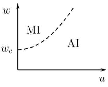
interactions. Chapter 4 contains a study of effects of Gaussian disorder on

the Mott-insulating state. We show that the intermediate Mott-glass state

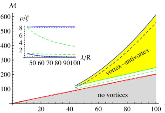
does not appear, in contrast to some studies. In chapter 5 we calculate the

ground state configurations of vortices in the film when a small ferromagnetic

dot is placed on the top of the film. In chapter 6 we show that a system that

consists of a superconducting film covered by magnetic dots with random

magnetization maps to the two-dimensional XY model and infer its phase

diagram.

11

Chapter 2

Transport in a Luttinger liquid with dissipation

In this chapter we study electron transport through a single impu- rity in a one-channel Luttinger liquid coupled to a dissipative Ohmic bath. For nonzero dissipation, the single impurity is always a relevant perturbation and suppresses transport strongly.

2.1 Introduction

The physics of a particle coupled to a dissipative environment is a funda- mental problem [32, 33]. Such theoretical model is realized in many different physical situations, which include damped motion of a particle in an external potential with thermal noise [34], tunnel junctions at low temperatures [35], motion of a heavy particle placed in a Luttinger liquid [36], and a supercon- ducting grain coupled to leads via Josephson junctions [37].

Common for the aforementioned systems is that they are problems of a single degree of freedom. A problem we are interested in is the electron tunneling through a single impurity placed in a Luttinger liquid. Since single particle excitations are absent in interacting one-dimensional systems, one would expect that our case belongs to a different class of problems. However, a closer look reveals that this is also a problem of a single particle; in our case this single particle is played by the fluctuating electron displacement field at the impurity position.

Our main concern in this chapter will be a question of transport in a Luttinger liquid with dissipation and a single impurity. While the Luttinger liquid state can be realized in a broad class of systems, see chapter 1 for some examples, we primarily consider quantum wires. In a one-dimensional quantum wire the transverse motion of electrons is quantized into discrete modes due to finite width of the wire, while the longitudinal motion is free.

For simplicity in the following we assume that just one transverse mode is

occupied.

12 Transport in a Luttinger liquid with dissipation

The wire is connected at its ends to Fermi-liquid leads which are reservoirs of electrons. When one lead has higher electrochemical potential than the other electrons propagate along the wire. If the applied field is an ac field of frequency ω, one obtains in the limit ω → 0 the two-terminal conductance G(ω → 0) = 2e ² /h, provided the length of the wire L obeys the condition L ≪ L ω = v/ω, where v denotes the plasmon (excitation) velocity [38, 39, 40]. On the contrary, for L ≫ L ω , one observes the low-frequency microwave conductance G(ω) < 2e ² /h.

In realistic cases electrons from the wire couple to other degrees of free- dom, e.g. to phonons or to electrons in nearby gates. It is usually the effect of screening of long-range Coulomb interaction between electrons due to gates which is considered for one-dimensional conductors [41]. Here we rather con- sider another effect: the dissipation. The electrons in the nearby gates are degrees of freedom which act as a dissipative bath for the electrons in the wire [32]. In particular, it has been shown recently that the coupling of the electrons from a clean wire to the electrons from surrounding metallic gates results in an Ohmic dissipation of the electrons in the wire [42].

The dissipation introduces a length scale L η . Above that length scale the electron motion is damped. While the electrons in quantum wires scatter of other electrons and of impurities (if they are present) elastically, the dissi- pative bath serves a source of inelastic scattering. Loosing their momenta in inelastic scattering events, the electrons dissipate energy of the system.

On physical grounds it means that the external dissipation increases the resistance of the wire, or equivalently decreases the conductance. What is important here is the ratio between wire’s length L and the dissipative length L η . Certainly, when L η ≫ L, the effect of the dissipation is very small and hence of no practical importance. In the opposite limit, L η ≫ L, the elec- tron motion in the wire is dominated by the dissipation and one expects that conductance is strongly reduced.

In addition, we are also interested in effects of an isolated impurity placed in the wire. The case without the dissipation is considered in a pioneering work by Kane and Fisher [19]. They found that impurity leaves the zero temperature conductance unchanged, provided the interaction is attractive.

This result is independent of the strength of the impurity. For repulsive interaction, on the other hand, the conductance vanishes at zero temperature as G ∼ V ^{2/K − 2} , where V is the applied voltage [19, 20, 21, 43]. At nonzero temperatures T and small voltages the conductance behaves as G ∼ T ^{2/K − 2} , remaining finite even for V → 0. This is due to thermally excited electrons which tunnel through the impurity.

The question that arises is: what is the influence of dissipation on the

transport properties of disordered Luttinger liquids? We address it in the

2.2 Model 13

rest of this chapter. In particular we study the influence of weak dissipation on the tunneling of electrons through a single impurity. This chapter is orga- nized as follows. In section 2.2 we introduce a model for interacting electrons in one dimension in the presence of a single impurity and dissipation. The model is analyzed in using the renormalization group method in section 2.3.

In section 2.4 we calculate the conductance of the system at finite voltage and temperature. In section 2.5 we calculate the decay of the mean elec- tron density, which is followed by conclusions. Some technical details are presented in appendix 2.A.

2.2 Model

We consider spinless electrons in a one-dimensional wire which are coupled to a dissipative bath. In the center of the wire of length L is a single δ- function like impurity of arbitrary strength. Following Haldane [44], the charge density ρ(x) can be rewritten as

ρ = k F

π − 1

π ∂ x ϕ + k F

π cos(2ϕ − 2k F x) + . . . , (2.1) where ϕ(x) denotes the bosonic (plasmon) displacement field and k _F is the Fermi wavevector. The Euclidean action of the system then reads [8]

S

~ = 1 2πK

Z L/2

− L/2

dx Z ^~ β/2

− ~ β/2

dτ 1

v (∂ τ ϕ) ² + v(∂ x ϕ) ² − 2πKW (ϕ)δ(x)

+ η 4

Z L/2

− L/2

dx Z ^~ β/2

− ~ β/2

dτ Z ^~ β/2

− ~ β/2

dτ ^′ [ϕ(x, τ ) − ϕ(x, τ ^′ )] ²

{ ~ β sin[π(τ − τ ^′ )/ ~ β] } ² , (2.2)

where β = 1/T . For K ≪ 1 Eq. (2.2) describes also a charge or spin density

wave, while K → 0 corresponds to the classical limit. W (ϕ) is the impurity

potential which is a periodic function of periodicity π. The last part in

the action (2.2) describes Ohmic dissipation [32]. It was derived from a pure

Luttinger liquid coupled electrostatically to a metallic gate in Ref. [42], where

it was found that such a coupling is only relevant for K < K η = 1/2. This

fact can be taken into account by writing η = η ₀ ξ _η ^{− 1} where ξ _η denotes the

Kosterlitz-Thouless correlation length diverging at the transition K → K η − 0

and η 0 is a dimensionless coupling constant. Since there may be other sources

of dissipation which survive also for K > 1/2, in the following we assume

that η > 0.

14 Transport in a Luttinger liquid with dissipation

In treating the influence of the impurity we first consider the zero tem- perature case. After Fourier transforming

ϕ(x, τ ) = Z dω

2π Z dk

2π ϕ k,ω e ^ikx+iωτ , (2.3)

the harmonic action reads S 0

~ = 1 2πK

Z dω 2π

Z dk 2π

1

v ω ² + vk ² + Kη | ω |

| ϕ k,ω | ² . (2.4) The last term of Eq. (2.4) describes the (weak) damping of the plasmons of complex frequency ω P ≈ v(k + i/(2L η )), where L η = 1/(Kη) is the dissi- pative length. The upper cutoff for momentum and frequency are Λ and ω c , respectively. ω _c = min { v Λ, E _diss / ~ } where E _diss corresponds to the maximal energy which can be dissipated by the dissipative bath. For simplicity we will assume that E diss > ~ vΛ, so that ω c = vΛ. Since the impurity acts at one point in space, the action is harmonic outside the impurity position.

One can then get an effective action by integrating out all degrees of freedom outside the impurity. Then, the resulting effective impurity action reads

S

~ ≈ 1 πK

Z dω 2π

p ω ² + Kvη | ω || φ _ω | ² − X ∞ n=1

w _n Z

dτ cos(2nφ), (2.5) where φ ω = R

dτ φ(τ )e ^{− iτ ω} and φ(τ ) ≡ ϕ(x = 0, τ ). Since W (φ) is a periodic function it is decomposed into a Fourier series in Eq. (2.5). As can be seen from Eq. (2.5), for low frequencies, ω < v/L η , the behavior of the system is controlled by the dissipation. For very large values of ω and sufficiently small dissipation, η ≪ Λ/K, the effective action (2.5) includes also a contribution

∼ R _dω

2π ω ² | φ _ω | ² [8], while in the opposite case of large dissipation, η ≫ Λ/K, it contains a term ∼ R _dω

2π | ω || φ ω | ² . This high frequency limit will be important for the analysis of the model in the strong impurity limit that we perform in the next section.

2.3 Renormalization group analysis

In the following we will perform a renormalization group analysis of the effec- tive model given by Eq. (2.5). For weak impurity strength we can calculate the renormalization of w n perturbatively. This gives for the flow equations of w n

dw _n

dl = 1 − n ² K p 1 + ηKe ^l /Λ

!

w n . (2.6)

2.3 Renormalization group analysis 15

There is no renormalization of K and η. This can already be argued from the fact that K and η are bulk quantities which cannot be renormalized by the local perturbation from the impurity. On a more formal level, one finds from integrating out the high frequency modes in Eq. (2.5) that one does not obtain terms depending in a nonanalytic way on frequency, see Refs. [19, 34].

For η = 0 we recover from Eq. (2.6) the result of Kane and Fisher [20], namely that the impurity is a relevant perturbation for repulsive interaction K < 1 and irrelevant for attractive interaction K > 1. As soon as the dissipa- tion is switched on, the downward renormalization saturates at a length scale l ^∗ given by e ^{l ∗} ≈ ΛL η . Thus the impurity is a relevant perturbation even for attractive interaction, provided the dissipation remains finite in this region.

If the dissipation results from the coupling to gate electrons, as considered in Ref. [42], η renormalizes to zero for K > 1/2 and hence the impurity potential renormalizes to zero for K > 1.

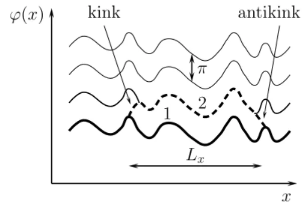
Motivated by the fact that a weak impurity flows toward strong impurity limit, we will consider now the system starting initially from very large im- purity strength. Then the cosine terms of impurity potential are important and the displacement field gets locked in their minima. The main contribu- tion to the partition function comes from configurations φ(τ) = nπ with n integer, interrupted by kinks which connect these pieces. These multi-kinks configurations are saddle points of the effective action (2.5). For very large impurity strength kinks are narrow, and hence are characterized by the high frequency limit of the action (2.5).

For sufficiently weak dissipation, η ≪ Λ/K, the resulting saddle point equation is the sine-Gordon equation in one dimension. It has a kink solution that interpolates between φ = nπ and φ = (n + 1)π in a narrow region of width δ ∼ 1/ √ w 1 . Outside that narrow region the solution very rapidly reaches the values φ = nπ and φ = (n + 1)π.

In the opposite case of strong dissipation, η ≫ Λ/K, the resulting saddle point equation is the sine-Hilbert (or Peierls-Nabarro called by some authors) equation [45, 46, 47]. As a difference from the sine-Gordon equation, it has a ‘nonlocal’ derivative of the displacement field R

dτ ^′ [φ(τ) − φ(τ ^′ )] /(τ − τ ^′ ) ²

instead of d ² φ/dτ ² . A kink solution for the sine-Hilbert equation is also

localized within a scale δ ∼ 1/ √ w ₁ , but as a difference from the sine-Gordon

case this solution has a long power law tail away from its center toward

values φ = nπ and φ = (n + 1)π. The important consequences of that

fact is a significant interaction energy between two kinks separated by a

distance d proportional to ln(L/d). For the sine-Gordon case this interaction

is exponentially small with the distance between kink centers and is negligible

for separations larger that the kink width. In the following we will consider

only the weak dissipation case.

16 Transport in a Luttinger liquid with dissipation

A saddle point solution φ s (τ ) of the effective action (2.5) with n kinks and n antikinks can be written as

φ s (τ ) ≈ π X 2n

i=1

ǫ i Θ(τ − τ i ), (2.7)

where ǫ i = ± 1 and kinks satisfy the electroneutrality condition P 2n

i=1 ǫ i = 0.

Θ(τ ) is the Heaviside step function and τ i are the kink positions. In frequency space the saddle point configuration can be written as

φ s,ω ≈ iπ ω

X 2n i=1

ǫ i exp(iωτ i ). (2.8)

We should emphasize that in addition to the interaction between kinks due the high frequency limit, exponentially small in the present case, an extra interaction is present due to the low frequency part of the quadratic part of the action (2.5). The low frequency part does not influence the shape of kinks, but contributes to the partition function. The partition function of the system is a sum over all possible saddle point solutions, and reads

Z = X ∞ n=0

X

ǫ j = ± 1

t ²ⁿ δ ²ⁿ (n!) ²

Z

dτ ₁ . . . dτ _2n exp

"

2 K

X

i<j

ǫ _i ǫ _j f (τ _i − τ _j )

#

. (2.9) Here t ∼ exp( − S kink / ~ ) is the tunneling transparency of the impurity and S kink ∼ √ w 1 denotes the action of an isolated kink. δ is a short time cutoff of the order of the kink width. The partition function (2.9) is valid in the dilute kink gas approximation [48] when the overlap of kinks is neglected.

The stronger the impurity is, the narrower the kink is and the smaller the tunneling transparency is. Then the dilute kink gas approximation is very well justified. The kink interaction is encoded into f (τ) and is given by the expression

f(τ ) = Z ω c

0

dω

p ω ² + vKη | ω |

ω ² [1 − cos(ωτ )] . (2.10)

In the limit of ω c τ ≫ 1 we obtain, up to an additive constant, an interpolating expression

f(τ ) ≈ ln ω c τ + p

2πvηKτ . (2.11)

The logarithmic interaction prevails for small kink-antikink distances τ, while

for larger τ the interaction exhibits a power law behavior. The different

2.4 Transport 17

behavior of f (τ) is very important and will determine different transport characteristics when one changes the external parameters (voltage or tem- perature).

A strong impurity can alternatively be considered as a weak link between the two half-wires x < 0 and x > 0, respectively. It is therefore convenient to rewrite the partition function (2.9) in a form in which t denotes the strength of the nonlinear terms. This can be done in the standard way, Refs. [21, 48], with the result Z = R

D θe ^{− S eff [θ]/ ~} with S eff

~ = K π

Z dω 2π

ω ²

p ω ² + vηK | ω | | θ ω | ² − 2t Z

dτ cos 2θ(τ ). (2.12) We can now consider the renormalization of t which is given by

dt

dl = 1 −

p 1 + ηKe ^l /Λ K

!

t. (2.13)

Again η ≡ 0 reproduces the known result of Ref. [20] that the weak link is renormalized to zero for K < 1. In the dissipative case the weak link is renor- malized to zero for all K provided η remains finite. Thus from Eq. (2.6) and Eq. (2.13) we conclude that the impurity is always a relevant perturbation.

2.4 Transport

So far we were concentrated on equilibrium properties. However, one is often interested in transport characteristics of the system. In this section we calculate the current I through the impurity when the voltage V is applied to the ends of the wire. Their ratio determines the conductance G = I/V .

In the case without impurity one may use the linear response theory [8].

In the limit of large system sizes L → ∞ and for low frequencies L ω ≫ L η

one gets finite conductivity σ(ω → 0) = ^e _h ² 2KL η . On the other hand for very weak dissipation, when L η ≫ L ω ≫ L, we know the result for the static con- ductance G = e ² /h. While in the former result the conductance of the wire is purely determined by the dissipation, in the latter case the dissipation is very weak and does not change the result for a clean quantum wire. Knowing the connection between the conductance G and the conductivity, which is in one dimension G = σ/L, one may write an interpolating expression for the static conductance

G = e ² h

1, L ≪ L η ,

2KL η

L , L ≫ L η . (2.14)

18 Transport in a Luttinger liquid with dissipation

In the case with impurity we have shown that impurity strength flows to large values. Under an applied external voltage electrons tunnel through the impurity. The tunneling rate Γ and hence the current follows from the expression [49]

~ Γ = 2T Im ln Z(V ), Z = Z 0 + iZ 1 , (2.15) where Z (V ) denotes the partition function in the presence of an external voltage. Z 0 includes the (stable) fluctuations of the φ field close to a local minimum φ = nπ, whereas Z 1 includes the voltage driven (unstable) fluc- tuations which connect neighboring minima φ = nπ → (n + 1)π. Since the strength of the impurity is renormalized to large values, we can use the sad- dle point approximation employed in the previous section for the calculation of Z. To obtain the saddle point action it is sufficient to consider a con- figuration consisting of a pair of kinks separated by a distance τ. Then we have

S(τ )

~ = 2

K f(τ ) + 2S kink

~ − eV

~ τ. (2.16)

Here we have taken into account that the voltage creates into the action (2.5) a term − eV R

dτ φ/( ~ π). Note that two-terminal voltage applied to the leads is, in general, different from the four-terminal voltage V which is relevant for tunneling. However, if the wire is not too long and the impurity is strong both voltages are approximately the same. The saddle point follows then from

2

K f ^′ (τ ) − eV

~ = 0. (2.17)

This gives for larger voltages for the saddle point τ c ≈ 2 ~ /(eV K) and hence for the current

I ∼ exp

− S(τ c )

~

∼ t ² eV

~ ω c

2/K

, eV ≪ ~ ω c . (2.18)

Taking into account quadratic fluctuations around the saddle point, we get an additional factor − 1 in the exponent in the previous formula, i.e. we reproduce the result of Kane and Fisher [20] for the conductance G ∼ (eV / ~ ω c ) ^{2/K − 2} . On the contrary, for smaller voltages we get for the sad- dle point τ c ≈ 2πηv ~ ² /(e ² V ² K) and hence

I ≈ A(V ) exp

− S(τ c )

~

= A(V )t ² exp

− C ¹ η κeV

, eV ≪ η

κ . (2.19)

2.4 Transport 19

From fluctuations around the saddle point one gets for the prefactor A(V ) ∼ (η/κ(eV ) ³ ) ^1/2 , while the numerical constant is C ¹ = 2. Here we have in- troduced the compressibility κ = K/(πv ~ ). The cross-over between regimes (2.18) and (2.19) happens at eV / ~ ≈ ηv. An independent calculation using the Fermi golden rule approach gives similar results, see appendix 2.A for more details.

In the case of non-interacting electrons κ coincides with the density of states. Then Eq. (2.19) can be obtained from the following argument: the probability that an electron tunnels over a distance r is proportional to P r(r) ∼ exp ( − 2r/L η ). To find the minimal r the number of states which can be reached has to be at least of the order one, i.e. κeV r ≈ 1. Inserting this into P r(r) gives Eq. (2.19) apart from a numerical factor.

As expected, the dissipation reduces the current with respect to the Kane- Fisher result strongly. This means that the tunneling density of states into the end of a semi-infinite Luttinger liquid with dissipation ρ end (E) is sup- pressed at low energies more than a power law found in the dissipation free case [20]. The current through the impurity may be written as

I ∼ t ² Z eV

0

dEρ end (E)ρ end (eV − E). (2.20)

Then using Eq. (2.19) we get ρ(E) ∼ exp

− C ¹ η 4κE

. (2.21)

Next we consider finite temperatures. In this case the extension of the τ axis is finite. Hence there will be a cross-over from Eq. (2.19) to a new behavior when the instanton hits the boundary, i.e. if τ c ≈ ~ /T . This eV to T dependence cross-over happens for eV ≈ T . For larger T the current is given by

I ≈ t ² B (T ) exp

"

− r C ² η

κT

#

V, T ≪ η

κ . (2.22)

The instanton calculation gives for the numerical constant C ² = 8. The prefactor B(T ) may be obtained from the Fermi golden rule approach, and is equal B(T ) ∼ T ^{− 2} (κT /η) ^1/4 . More details can be found in appendix 2.A.

In the dissipation free limit the conductance becomes G ∼ (T / ~ ω c ) ^{2/K − 2} .

A simple way to reproduce formula (2.22) follows from integration of the

flow equation for the transparency (2.13) and truncating the renormalization

20 Transport in a Luttinger liquid with dissipation

group flow at the thermal de Broglie wavelength ~ v/T of the plasmons [8].

This gives an effective tunneling transparency t eff ∼ t ~ vΛ

T exp

"

− r 4η

πκT

#

. (2.23)

The total current is then proportional to t ² _eff which agrees with result (2.22) apart from the value of C ² and the prefactor. Result (2.22) resembles variable range hopping in disordered quantum wires. Indeed, it can be written in the form I ∼ exp h

− p

C ² /(KκL η T ) i

V , which agrees with the variable hopping result if we replace L η by the correlation length ξ d of the disordered system [50]. This type of behavior has been indeed observed in quasi-one-dimensional La 3 Sr 3 Ca 8 Cu 24 O 41 , but attributed to variable range hopping [51].

2.5 Friedel oscillations

The presence of an impurity in a metal produces Friedel oscillations in the electron density [52]. The asymptotic form of the density in d ≥ 2 dimensions behaves as

ρ(x) ∼ cos(2k F x + ζ )

r ^d , (2.24)

where r is the distance from the impurity, k F the the Fermi vector and ζ is a phase shift. Effects of interactions in d ≥ 2 can be incorporated by Fermi liquid theory and does not change x ^{− d} decay. On the other hand in an interacting system in d = 1 dimension Fermi liquid theory breaks down.

There the decay is slower for repulsive interactions, and behaves as x ^{− K} , and faster for attraction K > 1, where behaves as x ^{1 − 2K} . It is obviously controlled by the interactions [53, 54].

In the present situation the dissipation is present and is expected to change the density profile at distances larger than L η , provided the sys- tem size is large enough. In this section we calculate the charge density oscillations. To determine the averaged charge density we write

h ρ(x) i = k F

π − 1

π h ∂ _x ϕ i + k F

π cos(2k _F x)e ^{− 2 h ϕ 2 (x) i} , (2.25)

where the average h . . . i is taken with respect to the full action (2.2). The

disorder average in the first term vanishes. To calculate the second term we

remark that in the presence of dissipation the impurity is always a relevant

perturbation and its strength grows under renormalization, see Eqs. (2.6)

2.6 Conclusions 21

and (2.13). To determine the large scale behavior of h ρ(x) i it is therefore justified to assume that ϕ is fixed at the defect. The fluctuation h ϕ ² (x) i is therefore identical to ¹ ₂ h (ϕ(x) − ϕ( − x)) ² i ⁰ , where h . . . i ⁰ is the average with respect to the quadratic action (2.4), see Ref. [47]. From this one finds

h ρ(x) i ∼ k F

π cos(2k F x) (

| x | ^{− K}

1+ _2πΛ ¹ _Lη

, x ≪ L η ,

1 + ^KL _{| x |} ^η , x ≫ L η . (2.26) For smaller distances x ≪ L η we get the well known power from Luttinger liquids, while for | x | ≫ L η the decay saturates.

2.6 Conclusions

In this chapter we have considered a Luttinger liquid model with Ohmic dissipation. In such a system on length scales larger than the dissipative length L η the elementary excitations (plasmons) become diffusive and the displacement fluctuations become strongly suppressed restoring translational long range order (some kind Wigner crystal, but not due to the unscreened Coulomb interaction [55]). For large system sizes the system gets finite con- ductivity, which is paralleled by diverging superfluid fluctuations. We have shown that weak dissipation has a dramatic effect on transport properties of a Luttinger liquid with a single impurity. The voltage and temperature dependence of the conductance is reduced from power laws in the dissipation free case to an exponential dependence, Eqs. (2.19) and (2.22), respectively.

2.A Conductance from the Fermi golden rule

In this appendix we will calculate the conductance for the system we have

introduced in this chapter using the Fermi golden rule approach. We closely

follow the paper by Furusaki and Nagaosa [21] where the conductance of a

Luttinger liquid with a single impurity is calculated. In our case the presence

of dissipation changes the quadratic part of the action, producing a change

in the conductance. For strong cosine potential the displacement field tend

to stay in one of the minima of the cosine from Eq. (2.5) at zero tempera-

ture. At finite temperature and finite small applied voltage the displacement

field tunnels to a neighboring minimum, because the applied voltage tilts the

potential landscape. The increase of the displacement field physically cor-

responds to the motion of electrons through the system due to the applied

voltage; this is expressed in terms of the conductance.

22 Transport in a Luttinger liquid with dissipation

Rather than working directly with the model (2.5) for strong impurity, we consider the problem in terms of an equivalent model which gives the same partition function, see Refs. [21, 56]. The equivalent model is given as a system of linear harmonic oscillators to which is coupled the single degree of freedom–in our case the displacement field φ(τ). Then calculating the voltage driven tunneling probability for the displacement field P φ 0 → φ 1 from where φ changes from φ 0 to φ 1 one gets the current I = e(P 0 → π − P π → 0 ) in the lowest order of the tunneling probability matrix element t. The final expression for the current reads [21]

I =et ²

1 − exp

− eV T

Z + ∞

−∞

dz cos eV

~ z

× (2.27)

exp

− π Z _∞

0

dω J(ω) ω ²

[1 − cos(ωz)] coth ~ ω

T

+ i sin(ωz)

, where

J(ω) = 2 πK

p ω ² + Kvη | ω | . (2.28)

Physically, the current is produced by the electron tunneling from one to another minimum of the cosine term which forms the potential landscape.

In the previous expression only the processes for tunneling into a neighboring minimum have been taken into account. In principle one should also take tunneling processes into the second (and higher order) nearest neighboring minimum, but these processes are expressed as higher powers of t and are neglected in Eq. (2.27).

The evaluation of Eq. (2.27) can be done in limiting cases when J(ω) ∼ | ω | and J (ω) ∼ | ω | ^1/2 . In the latter case by taking the exponential cutoff exp( − ω/(Kvη)) which mimics the frequency range where the dispersion comes purely from dissipation, one gets for T = 0 the result

I = 2πe ~ t ² exp 4

K − eV

~ Kvη

r η

κ(eV ) ³ exp

− 4η κeV

. (2.29)

In the former case again by taking the exponential cutoff exp( − ω/ω _c ) one gets

I = πet ²

ω c Γ(2/K) exp

− eV

~ ω c

eV

~ ω c

_K ² ₋ 1

. (2.30)

For nonzero temperatures one can also get the result for the conductance by evaluating expression (2.27). In the dissipative regime it reads

I ∼ ~ e ² t ² V T ²

κT η

1/4

exp

"

− r C 2 η

κT

#

, (2.31)

2.A Conductance from the Fermi golden rule 23

under the assumption eV ≪ T ≪ η/κ. For the numerical factor we get C ² = ⁹ ₄

16 √ 2 ζ(3/2)

2/3

≈ 9.49. For larger temperatures one gets the power law result

I ∼ e ² t ² V

~ ω ² _c T

~ ω c

2/K − 2

, (2.32)

which is the well known result for the conductance of a Luttinger liquid with

a single impurity at nonzero temperatures [19, 20].

This page intentionally left blank

25

Chapter 3

Realization of spin-polarized current in a quantum wire

In this chapter we consider an interacting quantum wire, modeled as a spinfull one-channel Luttinger liquid, placed in an external mag- netic field. For the case of two point-like impurities embedded in the wire, under a small voltage bias, the spin-polarized current occurs at special points in the parameter space, tunable by a single parameter.

Complete spin-polarization may be achieved at sufficiently low temper- atures, provided repulsive interactions are not too strong.

3.1 Introduction

In quantum mechanics it is well known that a one-dimensional plane wave incident on a high potential barrier is always partially transmitted. This effect is called quantum tunneling and does not exist in classical physics.

When the same plane wave impinges on a symmetric double barrier, it can be completely transmitted. This surprising effect occurs only for certain wavevectors, otherwise the plane wave is partially reflected and partially transmitted. This phenomenon, when the double barrier is transparent, but the individual one is opaque, is called resonant tunneling [57]. In optics, this phenomenon is in essence of a Fabry-P´erot interferometer, made of two parallel highly reflecting mirrors. Its transmission spectrum as a function of wavelength of incident light exhibits peaks of high transmission corre- sponding to resonances. The resonance tunneling effect can be explained as destructive interference of all reflected partial waves from the two barriers, leading to perfect transmission.

In addition to its wave nature, an electron has a charge. Therefore, the

electron transport in interacting one-dimensional systems is affected by the

Coulomb interaction. This is strikingly seen when a potential barrier, created

by a point impurity, is present in the system. When a voltage is applied at the

ends of the system, the impurity reflects (backscatters) electrons pushed by

the voltage, and tends to suppresses the transport. The conductance, which

26 Realization of spin-polarized current in a quantum wire

is proportional to the transmission of electrons, vanishes with the voltage for any strength of repulsive interaction [19, 20].

When two point impurities are present in the system, they make an island.

Knowing the physical picture of the single barrier, one would naively expect that the conductance of electrons is again strongly suppressed. However, this is not generally the case since the resonant tunneling effect also exists in the present situation. It explains perfect transmission through the island under some conditions. We can obtain them using a simple reasoning [8, 20], as will be explained now.

For weak impurities, the electron displacement field is just slightly per- turbed by them and tends to be constant in order to minimize the energy.

The condition for resonant tunneling follows from the requirement that the lowest harmonic of the electron density, that couples to the impurity poten- tial, vanishes. For not too strong repulsion this leads to perfect transmission.

In the opposite case, higher order harmonics of the electron density become important and destroy the resonance.

Direct tunneling through both impurities has very low probability, when

the impurities are strong. Rather, the process of sequential tunneling is

important. Strong impurities do not allow the leakage of charge under a small

applied voltage, and the island has a well defined charge on it. In the ground

state, this charge is fixed to an integer, which is determined by the position

of the Fermi level. An empty state on the island is important for sequential

tunneling. The process of electron transfer to the island is penalized by the

electrostatic energy, that occurs due to the existence of electrons at the island

which fill the energy states below the Fermi level. This process, when the

host electrons prevent the other to enter the island, is known as the Coulomb

blockade. However, when the distance between the impurities, or the gate

voltage at the island, is such that the states on the island that differ by one

electron become degenerate in energy, the Coulomb blockade is lifted. Under

such circumstances, an electron can enter the island from one side and then

leave at the other. While the Coulomb blockade does not hinder such process,

the barrier strength does. Knowing that the barrier strength is irrelevant

quantity for sufficiently strong quantum fluctuations in the system with a

single barrier, we expect the same in the present case. Quantum fluctuations

in these systems are measured by the Luttinger parameter K, which also

measures the interaction strength. It turns out that the critical value of K ,

when the two barriers become irrelevant, is inside the region of repulsive

interaction. This makes the effect of resonant tunneling of interacting one-

dimensional electrons more realistic and interesting. The resonant condition

in both limits of strong and weak impurities is the same, cos(k _F a) = 0. Here,

k F is the Fermi wavevector and a is the distance between impurities.

3.1 Introduction 27

Until now we considered spinless electrons. Including the electron spin degree of freedom, there will be no differences for weak impurity strengths.

Again, there is perfect transmission for not too strong repulsion, when a single parameter, such as the distance between impurities or the voltage on the island, is tuned [20]. However, important differences appear in the large-barrier limit. Resonant tunneling is also possible in that case, but the interpretation of this effect is different than in the spinless case and is based on the Kondo effect. When the number of electrons on the island is an odd integer, the spin on the island is degenerate. Then, the electron from the island may tunnel out of it, being replaced by an electron which enters from outside and which has opposite spin. In such way the electrons may be transferred through the island at no energy cost. The resulting current is non-spin-polarized due to SU(2) spin symmetry. In contrast to resonances in the spinless case when the charge state on the island is required to be degenerate, in the case with spin is needed a degenerate spin state. For electrons with spin, the aforementioned “charge” resonance mechanism is also possible, but requires more than one parameter to be tuned. Hence, it is difficult to achieve such resonances in practice.

Switching on a magnetic field, the electron spin symmetry is broken.

Electrons having different spin projections on the direction of the magnetic field become different particles, having different Fermi momenta and differ- ent spin. Assuming the field is not too strong to completely polarize the system, there are four Fermi points instead of two. The resonant tunneling phenomenon occurs for certain momenta of incident particles for a fixed dis- tance between the impurities. In the case with magnetic field, electrons of one spin direction can fulfill the resonance condition, while electrons having the other spin direction need not. This simple observation leads to the ap- pearance of a spin-polarized current in the case of non-interacting electrons at low temperatures under a small voltage bias at the ends of the system.

In literature little attention has been devoted to the question of trans- port in Luttinger liquids in an external magnetic field. Theoretical studies have shown that spin-polarized current may occur due to a strong degree of electron polarization [58], spin-dependent interactions [59], a large Fermi velocity difference of electrons having different spin [60, 61] or due to a mag- netic impurity [62]. Spin-orbit interaction in combination with a magnetic field may also enhance the degree of current polarization [63, 64, 65].

In contrast to the previous studies, we take into account neither Fermi

velocity asymmetry nor strong electron polarization. Rather, our study is

based on the phenomenon of resonant tunneling. By tuning a single parame-

ter, that changes the Fermi wavevector, we can reach a point where the reso-

nance condition is achieved for only one spin direction in the interacting case.