ALEPH,L3andOPALCollaborations .TheLEPWorkingGroupforTwo-PhotonPhysics ComparisonofDeepInelasticElectron-PhotonScatteringDatawiththeHerwigandPhojetMonteCarloModels

arXiv:hep-ex/0010041v1 17 Oct 2000

EUROPEAN ORGANISATION FOR NUCLEAR RESEARCH

CERN-EP-2000-109 July 3, 2000

Comparison of Deep Inelastic Electron-Photon Scattering Data with the Herwig and Phojet Monte

Carlo Models

ALEPH, L3 and OPAL Collaborations ¹ .

The LEP Working Group for Two-Photon Physics ²

Abstract

Deep inelastic electron-photon scattering is studied in the Q

range from 1.2 to 30 GeV

using the LEP1 data taken with the ALEPH, L3 and OPAL detectors at centre-of-mass energies close to the mass of the Z boson. Distributions of the measured hadronic final state are corrected to the hadron level and compared to the predictions of the HERWIG and PHOJET Monte Carlo models. For large regions in most of the distributions stud- ied the results of the different experiments agree with one another. However, significant differences are found between the data and the models. Therefore the combined LEP data serve as an important input to improve on the Monte Carlo models.

Submitted to European Physical Journal C

1For the members of the Collaborations see for example [1, 3, 4]

2 Contributions from P. Achard, V. Andreev, S. Braccini, M. Chamizo, G. Cowan, A. De Roeck, J.H. Field, A.J. Finch, C.H. Lin, J.A. Lauber, M. Lehto, M.N. Kienzle-Focacci, D.J. Miller, R. Nisius, S. Saremi, S. S¨oldner-Rembold, B. Surrow, R.J. Taylor, M. Wadhwa and A.E. Wright.

1 Introduction

The measurement of the hadronic structure function F

crucially depends on the ac- curate description of the hadronic final state by Monte Carlo models. The available models do not properly account for all features observed in the data, and therefore, at present, the accuracy of the measurement of F

is mainly limited by the imperfect description of the hadronic final state by the Monte Carlo models. In previous analyses of the individual LEP experiments [1–4], it had been shown that there are discrepancies in several distributions of the hadronic final state between the various QCD models and the data. It has also be seen that the data are precise enough to further constrain the models. The purpose of this paper is to combine the ALEPH, L3 and OPAL data to establish a consistent and significant measurement, which can be used to optimise the models.

In this paper the reaction e

e

→ e

e

γ

γ → e

e

hadrons, proceeding via the exchange of two photons, is studied in the single tag configuration, where one scattered electron

is detected. The differential cross-section for the deep inelastic electron-photon scattering reaction, e(k) γ(p) → e(k

) γ(p) γ

(q) → e X, where the terms in brackets denote the four-momentum vectors of the particles, is proportional to F

(x, Q

) [5]. Here Q

= − q

= − (k − k

)

and x = Q

/2p · q. Experimentally, in the single tag configuration, the value of x is obtained using

x = Q

Q

+ W

, (1)

where W

is the hadronic invariant mass squared, and P

= − p

is neglected in calcu- lating x.

The hadronic structure function F

receives contributions both from the point-like part and from the hadron-like part of the photon structure. The point-like part can be calculated in perturbative QCD. At low Q

the hadron-like part is usually modelled based on the Vector Meson Dominance model. The combined contributions are evolved using the DGLAP evolution equation.

Combining the results of three of the LEP experiments not only reduces the statis- tical errors compared to the individual results, but the difference between the results also gives a reliable estimate of the systematic, detector dependent, errors. The ex- perimental data are fully corrected for trigger inefficiencies and background has been subtracted. The experimental distributions presented are also corrected for detector effects using different Monte Carlo models, and can directly be compared to the model predictions based on generated quantities only, i.e., without the simulation of the de- tector response, provided that a well defined set of hadron level cuts defined below is applied. This experimental information serves as a basis for improvements on the models.

A set of variables is chosen to compare the corrected data to the hadron level predictions of the Monte Carlo models. The variables used are:

• the reconstructed invariant hadronic mass, W

, within a restricted range in polar angles with respect to the beam axis,

• the transverse energy out of the plane defined by the beam direction and the direction

3Electrons and positrons are referred to as electrons.

of the tagged electron, E

,

• the number of charged particles, N

,

• the transverse momenta of charged particles with respect to the beam axis, p

,

• and the hadronic energy flow, 1/N · d E/d η, as a function of the pseudorapidity η =

− ln(tan(θ/2)) with respect to the beam axis, where N denotes the number of events.

The complete definition of how these variables are calculated is given in Section 3.

For W

, E

and N

the result is a differential event cross-section, which means, the distributions have one entry per event, whereas for p

the distribution is a one- particle inclusive cross-section. The hadronic energy flow is shown as an average energy flow per event,

E/N , where the sum runs over all objects and over all events in a given bin of pseudorapidity.

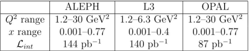
The analysis presented here is based on data of the individual experiments taken at centre-of-mass energies close to the mass of the Z boson. The approximate ranges in Q

and x of the different experiments used in this analysis, and the integrated luminosities are listed in Table 1. The Q

ranges are calculated from the requirements on the energy and angle of the deeply inelastically scattered electron, and the x ranges are derived from Eq. 1, using the range in Q

and the approximate reach in hadronic invariant mass of 3 < W < 35 GeV.

ALEPH L3 OPAL

Q

range 1.2–30 GeV

1.2–6.3 GeV

1.2–30 GeV

x range 0.001–0.77 0.001–0.4 0.001–0.77

L

144 pb

140 pb

87 pb

Table 1: The approximate ranges in Q

and x of the different experiments and the integrated luminosities L

used in this analysis.

2 Monte Carlo Models

The two Monte Carlo models studied are HERWIG5.9 [6] and PHOJET 1.05c [7], using the leading order GRV [8] parton distribution functions.

In the HERWIG model the hard interaction is simulated as e q → e q scattering,

where the incoming quark is generated according to a set of parton distribution func-

tions of the photon. The incoming quark is subject to an initial state parton shower

which contains the γ → q q vertex, and the outgoing partons undergo final state parton

showers as in the case of e

e

annihilations. The hadronisation is based on the cluster

model. The initial state parton shower is designed in such a way that the hardest emis-

sion is matched to the sum of the matrix elements for the resolved processes, g → q q,

q → q g and the point-like γ → q q process. The parton shower uses an angular evolu-

tion parameter, and so it obeys angular ordering. For point-like events the transverse

momentum of the partons with respect to the direction of the incoming photon is given

by perturbation theory. In contrast, for hadron-like events, the photon remnant gets a

transverse momentum k

with respect to the direction of the incoming photon, where

originally the transverse momentum was generated from a Gaussian distribution.

The HERWIG version used for event simulation is HERWIG5.9+k

, where the label k

denotes that the k

distribution has been altered from the program default. This change is made to improve the agreement for the high-Q

region between the ALEPH and OPAL data and the original HERWIG prediction, where the original program is denoted as HERWIG default. The default Gaussian behaviour is replaced by a power-law function of the form dk

/(k

+ k

) [9] with k

= 0.66 GeV. The change is motivated by the observation made in photoproduction studies at HERA [10], where the power-law function gave a better description of the data. This is a good example of how information from two different, but related reactions can be used to improve on a general purpose Monte Carlo program. It is interesting to note that the same value of k

is chosen to describe both, photoproduction and deep inelastic electron-photon scattering events. The upper limit of k

in HERWIG+k

is fixed at k

= 25 GeV

, which is almost the upper limit of Q

for the Q

region studied, as shown in Table 1.

Based on the distributions presented in Section 5 the fixed cut-off has been replaced by dynamically adjusting the upper limit on k

on an event by event basis [11]. In this scheme the maximum transverse momentum k

is set to the hardest virtuality scale in the event, which is of order Q

. The distributions produced with this procedure are denoted as HERWIG+k

(dyn).

The PHOJET Monte Carlo is based on the Dual Parton Model [12]. It is designed for hadron-hadron, photon-hadron and photon-photon collisions, where originally only real or quasi-real photons were considered. It has recently been extended to simulate the deep inelastic electron-photon scattering case, where one of the photons is highly virtual. For the case of deep inelastic scattering the program is not based on the DIS formula using F

, but the γ

γ cross-section is calculated from the γγ cross-section by extrapolating in Q

on the basis of the Generalised Vector Dominance model. The events are generated from soft and hard partonic processes, where a cut-off of 2.5 GeV on the transverse momentum of the scattered partons in the photon-photon centre- of-mass system is used to separate the two classes of events. The hard processes are sub-divided into direct processes, where the photon as a whole takes part in the hard interactions, and resolved processes. In resolved processes either one or both photons fluctuate into a hadronic state, and a quark or gluon of one hadronic state interacts either with the other photon, or with a quark or gluon of the second hadronic state.

Also virtual photons can interact as resolved states, however, the parton distribution functions of the photons are suppressed as a function of the photon virtualities. The sum of the processes is matched to the deep inelastic scattering cross-section. Initial state parton showers are simulated with a backward evolution algorithm using the transverse momentum as evolution scale. Final state parton showers are generated with the Lund code JETSET [13]. Both satisfy angular ordering implied by coherence effects.

The hadronisation is based on the Lund string model as implemented in JETSET.

3 Experimental Method

Large data sets are generated with the PHOJET and HERWIG+k

programs respec-

tively, for √ s = M

. All unstable particles with lifetimes of less than 1 ns are allowed

to decay in the event generation. In this way the particles of the final state correspond

approximately to those actually seen in the detectors. The corresponding integrated

luminosities for the PHOJET and HERWIG+k

samples are 831 pb

and 683 pb

respectively

.

The definitions of the phase space and observables include cuts at generator level both on the events and on the particles within the events. The cuts are chosen such that the individual detectors have good acceptance and therefore detector related un- certainties are expected to be small. To select the events at this stage, the following cuts are applied to the generated hadron level quantities:

1. The energy of the deeply inelastically scattered electron has to be larger than 35 GeV.

2. The polar angle θ

of the deeply inelastically scattered electron with respect to either beam direction has to be in the ranges 27 − 55 mrad (low-Q

region) or 60 − 120 mrad (high-Q

region). The two ranges in scattering angles studied correspond to Q

ranges of about 1.2 < Q

< 6.3 GeV

and 5.7 < Q

< 30 GeV

. 3. The events are required to contain no electron with energy of more than 35 GeV and polar angle above 25 mrad with respect to the beam direction in the hemi- sphere opposite to the one containing the deeply inelastically scattered electron.

4. The number of charged particles N

, calculated by summing over all charged particles which have a transverse momentum p

with respect to the beam axis of more than 200 MeV and polar angles, θ, with respect to the beam axis, in the range 20 < θ < 160

, has to be greater than or equal to 3. The values chosen closely resemble the acceptance of the tracking detectors.

5. The invariant mass W

, calculated by summing over all charged and neutral particles fulfilling p

> 200 MeV and 20 < θ < 160

, corresponding to | η | < 1.735, has to be larger than 3 GeV.

This set of particles and cuts defines the hadron level and the data are corrected to this level. The hadron level predictions of W

and E

are calculated from the charged and neutral particles defined above, and the distributions of N

and p

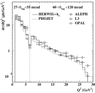
from the charged particles alone. The only exception is the hadronic energy flow. For the hadronic energy flow, the same event selection has been applied, but all particles are included in the distribution without applying a cut on transverse momentum. Figure 1 shows the differential cross-section dσ/dQ

within the cuts listed above and corrected for detector effects. The vertical line roughly separates the low- Q

and high-Q

regions. Since Q

depends on the energy and angle of the deeply inelastically scattered electron there is a slight overlap in Q

, but due to the cut on θ

the two samples are statistically independent. In the kinematic region studied the cross-section prediction of HERWIG+k

is about 40% higher than the prediction based on PHOJET as shown in Figure 1.

To study the experimentally observable distributions at the detector level samples of 60k HERWIG+k

and 120k PHOJET events, which are statistically independent from the samples mentioned above, are passed through the detector simulation programs of the ALEPH, L3 and OPAL collaborations, ensuring that all experiments use identical events. The objects reconstructed after the detector simulation are energy clusters, measured in the electromagnetic and hadronic calorimeters, and tracks, measured in

4The hadronisation parameters used for the PHOJET and HERWIG+k_t simulation have been determined from hadronic decays of theZ boson by the L3 [14] and OPAL [15] collaborations respec- tively.

the tracking devices. Identical event selection cuts at the detector level are applied by all experiments, closely reflecting the cuts applied at the hadron level as described above:

1. A cluster of at least 35 GeV is required in one of the small angle electromagnetic luminosity monitors.

2. The polar angle with respect to either beam direction of the cluster has to be in the range from 27 − 55 mrad or 60 − 120 mrad.

3. The most energetic cluster in the hemisphere opposite to the tagged electron has to have energy less than 35 GeV.

4. At least 3 tracks, fulfilling a set of quality criteria, are required to be observed in the tracking devices with 20

< θ < 160

, and with p

of at least 200 MeV.

5. The invariant mass, W

, calculated from all tracks and clusters with p

>

200 MeV and 20 < θ < 160

is required to be greater than 3 GeV.

These objects define the detector level. They are used for the W

, E

, N

and p

distributions. The only exception is the energy flow 1/N · d E/d η, where again no cut on the transverse momentum has been applied.

With this strategy it is ensured that the hadron level distributions, which are ob- tained from the large size samples without detector simulation, and the detector level distributions, which are obtained from the samples of smaller size with a detailed de- tector simulation for each individual experiment, are statistically independent. Both samples are used in the correction procedure applied to the data described in the next section.

4 Corrections for Detector Effects

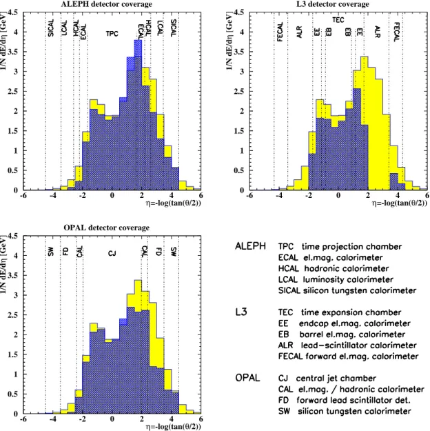
Before a measured quantity can be compared to theoretical predictions or to the results of other measurements it must first be corrected for various detector related effects, such as geometrical acceptance, detector inefficiency and resolution, decays, particle interactions with the material of the detector and the effects of the event and track selections. Figure 2 shows the energy flow, 1/N · d E/d η, predicted by the HERWIG+k

model at the hadron level as well as at the detector level, for the three detectors. The events are entered in the figure such that the deeply inelastically scattered electron is always at negative rapidities, but not shown. Also shown in the figure is the coverage in η of the various sub-detectors used in this analysis. A detailed description of the ALEPH, L3 and OPAL detectors can be found in [16], [17], and [18] respectively. The central region of all the detectors with − 1.735 < η < 1.735 is covered by tracking and calorimetry. The forward η > 1.735, and backward η < − 1.735 regions are covered by electromagnetic calorimeters for luminosity measurements and typically extend out to η = ± 4.3. The electromagnetic calorimeter of L3 between 1.735 < | η | < 3.411 is not used in the present analysis.

For the analysis presented here, the correction of the data to the hadron level is done with multiplicative factors, f, relating the measured value X

of a quantity X, such as a bin content, to the corrected value, X

using the relation:

X

= X

· f = X

· X

X

. (2)

For distributions, the correction factors are computed bin by bin, e.g. for the energy flow, f is the ratio of the hadron level (lightly shaded) and the detector level (darkly shaded) distributions shown in Figure 2. In this way of correcting the data the as- sumption is made that within the restricted angular range there is little smearing of the variables between bins, hence a simple correction factor is justified, and therefore no attempt to use an unfolding procedure has been made. The Monte Carlo was used to verify the accuracy of this assumption. Application of this correction results in measurements corrected to a well-defined kinematical region and particle composition, as defined in Section 3.

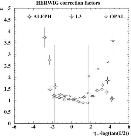
The correction factors for the energy flow in the low-Q

region are shown in Fig- ure 3. The correction factors are near one in the central region of pseudorapidity where identical cuts have been applied and they are similar for the three experiments. How- ever, there is a much larger spread in the region of larger pseudorapidity η > 1.735, where the experiments have different sub-detectors, different angular coverage, and apply different cuts. For ALEPH and OPAL the clusters in the forward detectors are required to have an energy of at least 1 GeV, while for L3 this requirement is at least 4 GeV. This leads to larger correction factors for L3 in that region. In addition, for L3, the clusters measured in the forward detectors on the side of the tagged electron, i.e. at η < − 2, are not considered in this study. Another difference in the treatment of clusters measured in the forward detectors is that OPAL uses a correction function, obtained from Monte Carlo studies of the detector response to hadrons, to correct for losses in the measurement of the hadronic energy in the forward detector, thereby also reducing the correction factors. It should be stressed that for most of the distribu- tions used for the comparisons in the following section, only the central detector part for polar angles with respect to the beam axis in the range 20 < θ < 160

, that is

| η | < 1.735, is exploited. The only exception is the energy flow where no cuts on the angle are applied.

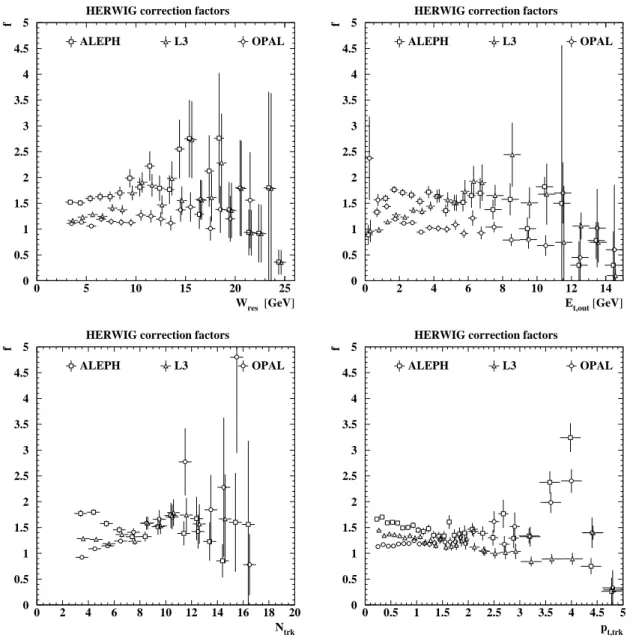
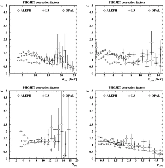
The correction factors in the low-Q

region for the other chosen variables and for the ALEPH, L3 and OPAL experiments using the HERWIG+k

and PHOJET mod- els, are shown in Figures 4 and 5. The quoted errors of the correction factors are the combined statistical uncertainties of the generated hadron level and the simu- lated detector level quantities. While the differences between the correction factors obtained from HERWIG+k

and PHOJET are very small for the energy flow, they can vary significantly for other variables. For example, in the case of OPAL, for W

the HERWIG+k

correction factors are on average about 20% higher than the factors obtained with PHOJET. The correction factors for the low-Q

and high-Q

regions typically differ by less than 10%.

5 Corrected Data Comparisons

The discussion of the comparison is subdivided into three parts. First the corrected data from the individual experiments are compared to each other and to the Monte Carlo models. In this comparison only statistical errors are used and no attempt has been made to obtain estimates of systematic errors for the individual experiments.

Based on the above comparison a modified version of the HERWIG+k

model has been

developed which is described next. Finally the data are combined and compared to the

Monte Carlo models. In the combination of the data the spread of the experiments is used as an estimate of the systematic uncertainty of the measured distributions. The numerical results are listed in Tables 2–12 and can be obtained in electronic form [19].

5.1 Data from individual experiments

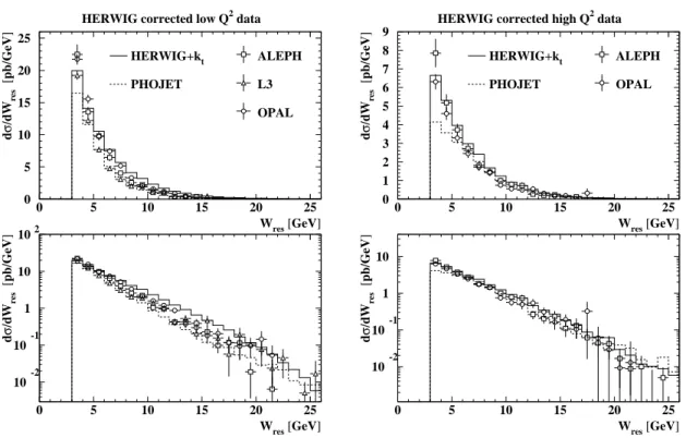
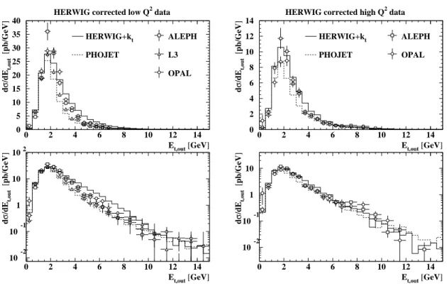
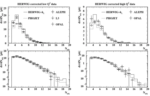
The Figures 6–13 show the corrected differential cross-sections, calculated in the kine- matical range described in Section 3, for the data compared with the HERWIG+k

and PHOJET predictions. Figures 6, 8, 10 and 12 show the data on a linear and log- arithmic scale, corrected with the HERWIG+k

model, while Figures 7, 9, 11 and 13 show the same data corrected with PHOJET. For all distributions the errors shown are the quadratic sum of the statistical errors of the measured quantity and the statistical errors of the correction factors. As an example, Table 2 shows the results for the W

distribution for the three experiments, listing the statistical error on the data and the statistical error on the correction factors, f , separately.

The experimental results from ALEPH, L3 and OPAL agree with each other within errors for large regions in most of the variables studied. However, there are also re- gions where they significantly differ from each other, for example, in the region of W

< 10 GeV, E

< 5 GeV, for low charged multiplicities and low p

in the low-Q

region. The level of agreement also depends on the Monte Carlo model used for correction. The agreement between the experiments is slightly better for the data corrected with PHOJET, than for the data corrected with HERWIG+k

. In the com- bination of the data, the differences between the measured distributions of the different experiments will be used as an estimate of the systematic error.

There are significant differences between the Monte Carlo distributions and the data, particularly in the low-Q

region. The PHOJET distributions lie consistently below HERWIG+k

, especially at the low end of the distributions, while the agreement of the tails in the high-Q

region is reasonable. In general the PHOJET predictions agree reasonably well with the data, corrected with PHOJET, for large values of the variables. However, there are large differences in the low-Q

region between the data, corrected with HERWIG+k

, and the HERWIG+k

predictions in all the distributions.

For the W

, E

and p

distributions (except in the region of low values, where the data are inconsistent) the differences between the experiments are much less than the HERWIG+k

− PHOJET differences.

Figures 14 and 15 show the corrected energy flow as a function of pseudorapidity in the low-Q

and high-Q

region for the individual experiments compared to the HERWIG+k

and PHOJET predictions. Following the energy flow analyses at HERA, the statistical errors for the energy flow are taken as √

E

/N . In Figure 14 the data are corrected with the HERWIG+k

model and in Figure 15 with the PHOJET model.

In the central region of the detector, between − 1.5 < η < 1.5, the data lie between the HERWIG+k

and the PHOJET predictions in the low-Q

region, whereas in the high- Q

region the two MC predictions lie closer to each other than the data of OPAL and ALEPH. These corrected energy flows in the central region are stable against changes in the requirements for the hadronic final state, e.g. changes to the quality cuts of the accepted tracks and clusters.

For η > 1.5 the data from the various experiments vary much more than the

statistical errors. Furthermore, it has been found that the corrected energy flows

are not very stable against variations of the event selection cuts such as the anti-tag condition or a maximum energy cut on the energy deposited in the forward detectors.

The observed changes are much larger at the detector level than at the hadron level, leading to the conclusion that the modelling of the energy response to the hadronic energy in the forward region is poor. This can be understood since the sub-detectors covering this region have poor energy resolution for hadronic energies and no particle identification. Therefore the uncertainty of the hadronic energy flow in the forward region is larger than is indicated by the spread of the experiments and it is difficult to draw firm conclusions on the description by the Monte Carlo models. However, the data appear to lie consistently below the prediction of either generator.

5.2 Modification of the HERWIG model

As discussed above, the distribution of transverse momentum k

of the photon remnant with respect to the direction of the incoming photon has been altered, motivated by the findings in photoproduction at HERA. At LEP, the modification was initially studied as a possible improvement of the agreement between the HERWIG prediction and the high-Q

data of OPAL and ALEPH. While HERWIG+k

seems to reasonably describe the data in the high-Q

region for low and high values of E

, it overestimates the distribution for medium values of E

, as shown in Figure 8. Even though the description of the energy flow is improved with the HERWIG+k

generator, it fails to accurately describe the data over a wide range of the pseudorapidity η.

While the fixed limit of k

= 25 GeV

is adequate for the high-Q

region, in the low-Q

region it introduces too much transverse momentum, which is most clearly seen in the transverse momentum distribution of the tracks in Figure 12. Therefore the dynamical adjustment, HERWIG+k

(dyn), as discussed in Section 2, has been introduced. As will be seen in the next section, when comparing with the combined LEP data, this change leads to an improved description of the data also for the low-Q

region.

5.3 Combined data

In this section the results from the individual experiments discussed in Section 5.1 are combined. In large ranges of the phase space the individual results agree within the statistical precision quoted, however there are also significant differences as discussed above. These differences are expected because the previous analyses of the individual LEP experiments [1–4] showed that the systematic errors, which are not included above, dominate. Because the Monte Carlo models do not sufficiently well resemble the data, evaluating the experimental systematic errors of the measurements based on these models will not be very reliable. On the other hand a combined result is desirable in order to serve as a guidance for the model builders to improve on their Monte Carlo programs. Therefore, in a first attempt to make a combined measurement, the experimental systematic error is taken from the spread of the measured results, wherever they are significantly different on the basis of the statistical error alone. In this case the purely statistical error of the combined result is inflated as discussed below.

The combined distributions from ALEPH, L3 and OPAL are shown in comparison

to PHOJET and various predictions from HERWIG in Figures 16–25. The measured values are listed in Tables 3–12. The combination of the data follows the procedure recommended by the Particle Data Group in section 4.2.2 of [20]. Since this is a crucial point of the analysis and because specific choices have to be made in the combination, the procedure is briefly discussed below.

The combined value for a given bin is calculated as the weighted average of the measurements of the individual experiments using the statistical errors to calculate both the weights and the error of the combined value. To calculate the average bin content x and its error σ

from the individual contents x

and their statistical errors σ

the following procedure is applied. The average content is calculated from x =

P

w

· x

/

w

, using the weights w

= 1/σ

. The sum runs over all experiments i = 1, . . . , N

with non-zero entries in that bin, and the error σ

is taken to be 1/ √

w

. The χ

of the average is calculated from χ

=

w

(x − x

)

. If in the tail of a distribution, for example, some experiments measure zero in a particular bin, then x and χ

are scaled by the ratio of the number of experiments with nonzero entries to the number of experiments being averaged for that bin. If χ

is larger than N

− 1, the error is increased by a factor S =

χ

/(N

− 1), thereby taking the spread of the experiments as an estimate of the experimental systematic uncertainty. Finally, to obtain the errors quoted the uncertainties due to the correction factors are added in quadrature. Since the same data sets are used by each experiment to calculate the correction factors, the corresponding errors are strongly correlated between the experiments. To take this into account, the error on the correction factors is included by taking the smallest quoted error of the individual experiments as an estimate of this systematic error, which is assumed to be 100% correlated amongst the experiments.

Also in the combination of the results of the individual experiments the 1/N · d E/d η distribution is treated slightly differently from the other distributions. There is a large scatter in the measured values of the different experiments, especially in the forward region, as can be seen from Figures 14 and 15. As a consequence there is also a large scatter in the scale factors listed in Tables 11 and 12. To avoid the combination proce- dure manufacturing artificially small errors for bins where the measurements happen to coincide, the scale factor applied to obtain the combined measurement is taken as the average of the individual scale factors from three neighbouring bins centered around the bin under study.

It is apparent from Figures 16, 18, 20, 22 and 24, that the new HERWIG+k

(dyn) with the dynamical cut-off lies much closer to the low-Q

averaged data than the version of HERWIG+k

using the fixed cut-off. However, the difference between HERWIG+k

(dyn) and HERWIG default is rather small.

In the case of the energy flow none of the various HERWIG models is able to accurately describe the data. This suggests that even though the new HERWIG+k

(dyn) better describes most of the data distributions, the energy flow is still not well understood.

The PHOJET model, Figures 17, 19, 21, 23 and 25, describes the data reasonably well in both regions of Q

, but underestimates the cross-section near the lower limit of the distributions. This is understood as a consequence of the high transverse momen- tum cut-off of 2.5 GeV for the scattered partons in the hard scattering matrix element.

Below this cut-off only soft events are generated. Due to the different Q

dependences

of the soft and hard components in PHOJET, this leads to a suppression of the low-W

events [21].

The energy flow corrected with HERWIG+k

and with PHOJET Figures 24 and 25, mostly agree with each other within errors, except in a few bins in the forward region.

In this region the data corrected with PHOJET lie below the data corrected with HERWIG+k

in the region of the peak at η ≃ 2 and above the flow corrected with HERWIG+k

in the region of η > 2.5.

6 Conclusion

For the first time the results of deep inelastic electron-photon scattering from three of the LEP experiments have been combined and compared to predictions from the PHOJET and the HERWIG models. It is found that the data from the ALEPH, L3 and OPAL experiments agree within statistical errors except near the edges of the distributions. Where the spread is larger than expected from the statistical errors, as, for example, for low charged multiplicities, this difference is taken as an estimate of the detector dependent systematic uncertainty of the measurement.

In the comparison of the data with the HERWIG+k

model the most striking discrepancy is seen in the distributions of the low-Q

region, where the HERWIG+k

model systematically overestimates the data. This discrepancy is found to be mainly due to the fixed cut-off for the intrinsic transverse momentum of the quarks in the photon in the HERWIG+k

model. By dynamically adjusting the cut-off according to the kinematics of the individual event in the HERWIG+k

(dyn) model the description of the data is significantly improved, particularly in the low-Q

region.

The PHOJET model describes the data reasonably well in both regions of Q

, but underestimate the cross-section near the lower limit of the distributions, due to the high transverse momentum cut-off for the scattered partons in the hard scattering matrix element.

The energy flow of the data lies between the predictions of the HERWIG and PHOJET Monte Carlo models in the central regions of the detectors. In the forward region the Monte Carlo predictions lie systematically above the data. It should be noted, however, that it is difficult to assess the systematic errors in this region be- cause of the poor resolution of the hadronic energy measured in the electromagnetic luminosity monitors.

The method of combining the data of several of the LEP experiments has proven useful to detect shortcomings of Monte Carlo models in the description of these data.

For the HERWIG Monte Carlo this investigation already demonstrated that the changed

distribution of transverse momentum k

of the photon remnant with respect to the di-

rection of the incoming photon, the HERWIG+k

(dyn) model, gives a better descrip-

tion of the LEP data. As the data distributions are corrected to the hadron level, they

can be directly compared to the predictions of the Monte Carlo models, without the

need of detector simulation, and thus can be used more easily by Monte Carlo model

builders.

Acknowledgements

We wish to thank R. Engel and M.H. Seymour for valuable discussions and useful

advice concerning the use of the Monte Carlo models.

References

[1] OPAL Collaboration, R. Akers et al., Z. Phys. C61 , 199–208 (1994);

OPAL Collaboration, K. Ackerstaff et al., Z. Phys. C74, 33–48 (1997);

OPAL Collaboration, K. Ackerstaff et al., Phys. Lett. B411, 387–401 (1997);

OPAL Collaboration, K. Ackerstaff et al., Phys. Lett. B412, 225–234 (1997).

[2] DELPHI Collaboration, P. Abreu et al., Z. Phys. C69, 223–234 (1996).

[3] L3 Collaboration, M. Acciarri et al., Phys. Lett. B436, 403–416 (1998);

L3 Collaboration, M. Acciarri et al., Phys. Lett. B447, 147–156 (1999).

[4] ALEPH Collaboration, D. Barate et al., Phys. Lett. B458 , 152–166 (1999).

[5] C. Berger and W. Wagner, Phys. Rep. 146, 1–134 (1987);

R. Nisius, Phys. Rep. 332, 165–317 (2000).

[6] G. Marchesini et al., Comp. Phys. Comm. 67, 465–508 (1992).

[7] R. Engel, Z. Phys. C66, 203–214 (1995);

R. Engel, J. Ranft, Phys. Rev. D54, 4246–4262 (1996).

[8] M. Gl¨ uck, E. Reya and A. Vogt, Phys. Rev. D45, 3986–3994 (1992);

M. Gl¨ uck, E. Reya and A. Vogt, Phys. Rev. D46, 1973–1979 (1992).

[9] J.A. Lauber, L. L¨onnblad and M.H. Seymour, Tuning MC Models to fit DIS eγ Scattering Events, in Proceedings of Photon ’97, 10-15 May 1997, eds A. Buijs, F.C. Ern´e, World Scientific, 52–56 (1997);

S. Cartwright, M.H. Seymour et al., J. Phys. G24, 457–481 (1998).

[10] ZEUS Collaboration, M. Derrick et al., Phys. Lett. B354, 163–177 (1995).

[11] M.H. Seymour, private communication.

[12] A. Capella, U. Sukhatme, C.I Tan, and J. Tran Thanh Van, Phys. Rep. 236, 225–329 (1994).

[13] T. Sj¨ostrand, Comp. Phys. Comm. 82, 74–89 (1994).

[14] L3 Collaboration, B. Adeva et al., Z. Phys. C55, 39–62 (1992).

[15] Available: http://www.ph.ed.ac.uk/ ˜ knowles/HW/hwtune.html, July 3, 2000.

[16] ALEPH Collaboration, D. Decamp et al., Nucl. Instr. and Meth. A294, 121–171 (1990), Erratum-ibid. A303 393 (1991);

ALEPH Collaboration, D. Buskulic et al., Nucl. Instr. and Meth. A360, 481–506 (1995).

[17] L3 Collaboration, B. Adeva et al., Nucl. Instr. and Meth. A289, 35–102 (1990);

L3 Collaboration, M. Acciarri et al., Nucl. Instr. and Meth. A351 , 300–312 (1994);

M. Chemarin et al., Nucl. Instr. and Meth. A349, 345–355 (1994);

I.C. Brock et al., Nucl. Instr. and Meth. A381, 236–266 (1996);

L3 Collaboration, A. Adam et al., Nucl. Instr. and Meth. A383 , 342–366 (1996).

[18] OPAL Collaboration, K. Ahmet et al., Nucl. Instr. and Meth. A305, 275–319 (1991);

P.P. Allport et al., Nucl. Instr. and Meth. A324, 34–52 (1993);

P.P. Allport et al., Nucl. Instr. and Meth. A346, 476–495 (1994);

B.E. Anderson et al., IEEE Transactions on Nuclear Science 41, 845–852 (1994).

[19] Available: http://home.cern.ch/LEPQCD/gamma gamma, July 3, 2000.

[20] C. Caso et al., Review of Particle Physics, Eur. Phys. J. C3, 1–794 (1998).

[21] R. Engel, J. Ranft, Phys. Rev. D54, 4246–4262 (1996);

R. Engel, private communication.

ALEPH L3 OPAL

W

[GeV] dσ/dW

[pb/GeV] dσ/dW

[pb/GeV] dσ/dW

[pb/GeV]

3 − 4 22.47 ± 1.378 ± 0.713 19.21 ± 0.405 ± 0.541 21.72 ± 0.535 ± 0.595 4 − 5 13.54 ± 0.560 ± 0.510 12.23 ± 0.332 ± 0.420 15.54 ± 0.457 ± 0.514 5 − 6 9.807 ± 0.553 ± 0.438 7.690 ± 0.270 ± 0.311 9.725 ± 0.352 ± 0.359 6 − 7 6.455 ± 0.441 ± 0.340 4.752 ± 0.210 ± 0.222 7.448 ± 0.325 ± 0.339 7 − 8 4.039 ± 0.239 ± 0.247 3.083 ± 0.181 ± 0.177 5.184 ± 0.266 ± 0.270 8 − 9 2.579 ± 0.181 ± 0.192 2.035 ± 0.146 ± 0.136 3.317 ± 0.213 ± 0.202 9 − 10 2.240 ± 0.177 ± 0.200 1.898 ± 0.155 ± 0.158 2.059 ± 0.167 ± 0.141 10 − 11 1.051 ± 0.118 ± 0.106 1.391 ± 0.143 ± 0.144 1.590 ± 0.155 ± 0.136 11 − 12 0.962 ± 0.126 ± 0.124 1.021 ± 0.117 ± 0.122 1.203 ± 0.135 ± 0.119 12 − 13 0.424 ± 0.073 ± 0.059 0.429 ± 0.067 ± 0.054 0.873 ± 0.113 ± 0.100 13 − 14 0.431 ± 0.073 ± 0.068 0.525 ± 0.087 ± 0.088 0.374 ± 0.071 ± 0.048 14 − 15 0.390 ± 0.083 ± 0.087 0.205 ± 0.053 ± 0.037 0.298 ± 0.072 ± 0.050 15 − 16 0.230 ± 0.066 ± 0.063 0.467 ± 0.101 ± 0.128 0.181 ± 0.061 ± 0.036 16 − 17 0.099 ± 0.030 ± 0.022 0.156 ± 0.042 ± 0.038 0.205 ± 0.064 ± 0.050 17 − 18 0.118 ± 0.042 ± 0.038 0.057 ± 0.040 ± 0.016 0.116 ± 0.037 ± 0.027 18 − 19 0.115 ± 0.054 ± 0.053 0.195 ± 0.056 ± 0.082 0.094 ± 0.044 ± 0.031 19 − 20 0.019 ± 0.014 ± 0.008 0.107 ± 0.032 ± 0.042 0.097 ± 0.037 ± 0.036 20 − 21 0.000 ± 0.000 ± 0.000 0.077 ± 0.031 ± 0.039 0.145 ± 0.055 ± 0.075 21 − 22 0.007 ± 0.007 ± 0.003 0.024 ± 0.013 ± 0.011 0.054 ± 0.031 ± 0.032 Table 2: The individual differential cross-section dσ/dW

in the low-Q

region for the ALEPH, L3 and OPAL data at √

s = 91 GeV, calculated in the kinematical range

defined in the text. The data have been corrected with HERWIG+k

. The first error

listed is the statistical error on the data only, the second one is the statistical error

arising from the correction factors, f.

low-Q

high-Q

HERWIG+k

MC Data MC Data

W

[GeV] h dσ/dW

i [pb/GeV] S h dσ/dW

i [pb/GeV] S

3 − 4 19.97 20.25 ± 1.064 2.887 6.651 6.557 ± 0.646 2.142

4 − 5 14.10 13.41 ± 1.097 4.146 5.304 4.787 ± 0.370 1.301

5 − 6 10.53 8.622 ± 0.792 3.628 3.961 3.510 ± 0.302 1.448

6 − 7 7.732 5.669 ± 0.875 5.115 2.979 2.575 ± 0.219 1.006

7 − 8 5.718 3.832 ± 0.626 4.680 2.411 1.764 ± 0.175 0.419

8 − 9 4.106 2.485 ± 0.385 3.534 1.682 1.444 ± 0.165 0.204

9 − 10 3.222 2.051 ± 0.172 1.028 1.243 0.854 ± 0.152 1.841

10 − 11 2.323 1.292 ± 0.195 2.040 0.915 0.658 ± 0.140 1.813

11 − 12 1.707 1.053 ± 0.127 0.957 0.733 0.595 ± 0.154 1.537

12 − 13 1.224 0.499 ± 0.129 2.570 0.459 0.318 ± 0.125 2.530

13 − 14 0.926 0.433 ± 0.071 0.953 0.345 0.231 ± 0.065 1.322

14 − 15 0.653 0.270 ± 0.069 1.366 0.267 0.193 ± 0.059 0.967

15 − 16 0.469 0.247 ± 0.087 1.726 0.180 0.136 ± 0.053 1.362

16 − 17 0.345 0.129 ± 0.040 1.202 0.139 0.114 ± 0.045 0.455

17 − 18 0.259 0.098 ± 0.032 0.874 0.086 0.078 ± 0.075 1.995

18 − 19 0.168 0.127 ± 0.051 1.023 0.064 0.047 ± 0.028 0.359

19 − 20 0.117 0.039 ± 0.029 2.134 0.061 0.039 ± 0.024 0.388

20 − 21 0.087 0.062 ± 0.020 1.117 0.029 0.013 ± 0.010 0.561

21 − 22 0.057 0.011 ± 0.009 1.287 0.020 0.009 ± 0.007 0.127

Table 3: The combined differential cross-section h dσ/dW

i calculated in the kine-

matical range defined in the text for the low-Q

and high-Q

regions. The data are

corrected with the HERWIG+k

model. The HERWIG+k

prediction (MC) and the

scale factor S are shown in addition.

low-Q

high-Q

PHOJET MC Data MC Data

W

[GeV] h dσ/dW

i [pb/GeV] S h dσ/dW

i [pb/GeV] S

3 − 4 16.47 19.06 ± 0.545 1.555 4.145 6.266 ± 0.594 2.025

4 − 5 11.55 13.12 ± 0.341 0.978 3.571 4.580 ± 0.306 0.897

5 − 6 7.704 8.447 ± 0.432 1.975 3.058 3.244 ± 0.225 0.471

6 − 7 5.078 5.601 ± 0.394 2.266 2.606 2.819 ± 0.261 1.322

7 − 8 3.399 3.532 ± 0.290 2.271 2.028 1.740 ± 0.163 0.691

8 − 9 2.115 2.124 ± 0.142 1.270 1.490 1.339 ± 0.139 0.391

9 − 10 1.405 1.531 ± 0.114 1.103 0.968 0.950 ± 0.182 2.052

10 − 11 0.858 0.875 ± 0.087 1.220 0.680 0.598 ± 0.090 0.629

11 − 12 0.581 0.623 ± 0.072 1.193 0.509 0.363 ± 0.073 1.164

12 − 13 0.366 0.323 ± 0.104 3.259 0.314 0.288 ± 0.066 1.183

13 − 14 0.266 0.254 ± 0.039 0.985 0.220 0.175 ± 0.041 0.267

14 − 15 0.215 0.160 ± 0.030 0.600 0.152 0.143 ± 0.044 0.270

15 − 16 0.119 0.102 ± 0.023 0.939 0.101 0.098 ± 0.055 2.301

16 − 17 0.087 0.084 ± 0.022 0.422 0.079 0.061 ± 0.023 0.452

17 − 18 0.086 0.065 ± 0.025 1.281 0.061 0.051 ± 0.022 0.036

18 − 19 0.054 0.042 ± 0.024 1.922 0.039 0.021 ± 0.011 0.035

19 − 20 0.045 0.044 ± 0.027 1.895 0.027 0.023 ± 0.018 1.339

20 − 21 0.028 0.037 ± 0.016 0.948 0.038 0.023 ± 0.017 0.443

21 − 22 0.030 0.016 ± 0.008 0.693 0.031 0.000 ± 0.000 0.000

Table 4: The combined differential cross-section h dσ/dW

i calculated in the kine-

matical range defined in the text for the low-Q

and high-Q

regions. The data are

corrected with the PHOJET model. The PHOJET prediction (MC) and the scale

factor S are shown in addition.

low-Q

high-Q

HERWIG+k

MC Data MC Data

E

[GeV] h dσ/dE

i [pb/GeV] S h dσ/dE

i [pb/GeV] S

0.0 − 0.5 0.521 0.266 ± 0.064 3.015 0.213 0.330 ± 0.227 3.043

0.5 − 1.0 7.221 6.201 ± 0.413 1.929 2.726 1.955 ± 0.262 0.733

1.0 − 1.5 20.73 18.97 ± 0.875 2.113 8.155 6.647 ± 0.907 2.282

1.5 − 2.0 27.75 28.04 ± 1.259 2.132 10.56 9.095 ± 1.070 2.214

2.0 − 2.5 24.38 23.54 ± 2.567 5.679 9.519 9.330 ± 0.712 1.585

2.5 − 3.0 18.34 15.91 ± 2.566 6.627 6.723 6.075 ± 0.393 0.928

3.0 − 3.5 13.12 9.316 ± 1.170 3.804 4.831 4.739 ± 0.369 0.630

3.5 − 4.0 9.595 6.182 ± 1.275 4.722 3.405 2.196 ± 0.213 0.653

4.0 − 4.5 7.048 4.481 ± 0.473 1.744 2.360 1.782 ± 0.202 0.665

4.5 − 5.0 4.939 2.286 ± 0.249 1.214 1.894 1.357 ± 0.174 0.409

5.0 − 5.5 3.680 2.020 ± 0.431 2.122 1.142 0.830 ± 0.132 0.572

5.5 − 6.0 2.855 1.341 ± 0.289 2.149 0.998 0.750 ± 0.148 1.238

6.0 − 6.5 2.131 1.035 ± 0.225 1.593 0.600 0.513 ± 0.108 0.258

6.5 − 7.0 1.446 0.545 ± 0.106 0.661 0.503 0.385 ± 0.112 0.769

7.0 − 8.0 0.937 0.376 ± 0.062 1.113 0.321 0.517 ± 0.068 1.922

8.0 − 9.0 0.488 0.246 ± 0.052 0.596 0.211 0.288 ± 0.045 1.051

9.0 − 10.0 0.234 0.093 ± 0.027 0.990 0.079 0.149 ± 0.034 1.055

10.0 − 11.0 0.095 0.067 ± 0.015 0.894 0.064 0.104 ± 0.042 0.000

11.0 − 12.0 0.066 0.058 ± 0.031 0.783 0.034 0.045 ± 0.016 0.629

12.0 − 13.0 0.037 0.005 ± 0.006 1.011 0.020 0.000 ± 0.000 0.000

13.0 − 14.0 0.025 0.012 ± 0.014 1.700 0.012 0.004 ± 0.003 0.835

14.0 − 15.0 0.022 0.001 ± 0.002 0.516 0.012 0.000 ± 0.000 0.000

Table 5: The combined differential cross-section h dσ/dE

i calculated in the kine-

matical range defined in the text for the low-Q

and high-Q

regions. The data are

corrected with the HERWIG+k

model. The HERWIG+k

prediction (MC) and the

scale factor S are shown in addition.

low-Q

high-Q

PHOJET MC Data MC Data

E

[GeV] h dσ/dE

i [pb/GeV] S h dσ/dE

i [pb/GeV] S

0.0 − 0.5 0.674 0.421 ± 0.064 2.348 0.216 0.451 ± 0.172 0.583

0.5 − 1.0 7.089 6.401 ± 0.251 1.772 2.465 2.090 ± 0.313 0.058

1.0 − 1.5 20.92 18.87 ± 0.602 2.629 6.629 6.298 ± 0.749 1.853

1.5 − 2.0 25.34 27.80 ± 0.822 1.827 8.616 9.388 ± 1.092 2.115

2.0 − 2.5 18.55 24.99 ± 1.028 1.885 6.576 8.496 ± 0.735 1.706

2.5 − 3.0 10.25 14.93 ± 0.930 2.176 4.438 5.730 ± 0.433 0.303

3.0 − 3.5 5.931 8.639 ± 0.791 2.505 3.031 4.147 ± 0.434 1.352

3.5 − 4.0 3.614 5.654 ± 0.482 1.607 1.996 2.105 ± 0.238 0.665

4.0 − 4.5 2.343 3.968 ± 0.331 1.129 1.490 1.522 ± 0.192 0.724

4.5 − 5.0 1.589 2.063 ± 0.205 0.611 1.127 1.316 ± 0.205 0.808

5.0 − 5.5 1.160 1.644 ± 0.222 1.156 0.874 0.825 ± 0.179 1.404

5.5 − 6.0 0.797 1.081 ± 0.175 1.413 0.594 0.789 ± 0.200 1.408

6.0 − 6.5 0.585 0.900 ± 0.216 1.826 0.493 0.419 ± 0.095 0.220

6.5 − 7.0 0.423 0.373 ± 0.073 0.803 0.375 0.371 ± 0.122 0.178

7.0 − 8.0 0.330 0.376 ± 0.063 1.866 0.250 0.235 ± 0.055 0.758

8.0 − 9.0 0.181 0.147 ± 0.045 1.854 0.151 0.138 ± 0.031 0.710

9.0 − 10.0 0.114 0.083 ± 0.015 0.596 0.088 0.134 ± 0.028 0.000

10.0 − 11.0 0.084 0.072 ± 0.022 0.280 0.073 0.018 ± 0.012 0.000

11.0 − 12.0 0.051 0.018 ± 0.009 0.515 0.057 0.055 ± 0.016 0.000

12.0 − 13.0 0.048 0.013 ± 0.013 1.410 0.034 0.000 ± 0.000 0.000

13.0 − 14.0 0.024 0.036 ± 0.018 0.509 0.019 0.000 ± 0.000 0.000

14.0 − 15.0 0.030 0.012 ± 0.017 0.174 0.019 0.000 ± 0.000 0.000

Table 6: The combined differential cross-section h dσ/dE

i calculated in the kine-

matical range defined in the text for the low-Q

and high-Q

regions. The data are

corrected with the PHOJET model. The PHOJET prediction (MC) and the scale

factor S are shown in addition.

low-Q

high-Q

HERWIG+k

MC Data MC Data

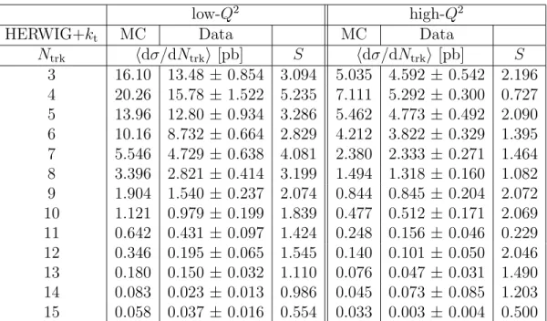
N

h dσ/dN

i [pb] S h dσ/dN

i [pb] S 3 16.10 13.48 ± 0.854 3.094 5.035 4.592 ± 0.542 2.196 4 20.26 15.78 ± 1.522 5.235 7.111 5.292 ± 0.300 0.727 5 13.96 12.80 ± 0.934 3.286 5.462 4.773 ± 0.492 2.090 6 10.16 8.732 ± 0.664 2.829 4.212 3.822 ± 0.329 1.395 7 5.546 4.729 ± 0.638 4.081 2.380 2.333 ± 0.271 1.464 8 3.396 2.821 ± 0.414 3.199 1.494 1.318 ± 0.160 1.082 9 1.904 1.540 ± 0.237 2.074 0.844 0.845 ± 0.204 2.072 10 1.121 0.979 ± 0.199 1.839 0.477 0.512 ± 0.171 2.069 11 0.642 0.431 ± 0.097 1.424 0.248 0.156 ± 0.046 0.229 12 0.346 0.195 ± 0.065 1.545 0.140 0.101 ± 0.050 2.046 13 0.180 0.150 ± 0.032 1.110 0.076 0.047 ± 0.031 1.490 14 0.083 0.023 ± 0.013 0.986 0.045 0.073 ± 0.085 1.203 15 0.058 0.037 ± 0.016 0.554 0.033 0.003 ± 0.004 0.500 Table 7: The combined differential cross-section h dσ/dN

i calculated in the kine- matical range defined in the text for the low-Q

and high-Q

regions. The data are corrected with the HERWIG+k

model. The HERWIG+k

prediction (MC) and the scale factor S are shown in addition.

low-Q

high-Q

PHOJET MC Data MC Data

N

h dσ/dN

i [pb] S h dσ/dN

i [pb] S 3 11.02 13.44 ± 0.893 3.457 3.514 4.594 ± 0.447 1.710 4 13.76 15.73 ± 1.022 3.556 4.800 5.392 ± 0.519 2.366 5 10.38 12.76 ± 0.536 1.890 3.878 4.207 ± 0.343 1.536 6 7.034 7.931 ± 0.713 3.801 3.202 3.537 ± 0.246 0.486 7 3.891 4.405 ± 0.443 3.180 2.025 2.031 ± 0.292 2.263 8 2.249 2.412 ± 0.321 3.147 1.319 1.385 ± 0.203 1.881 9 1.099 1.286 ± 0.172 2.151 0.735 0.805 ± 0.173 1.917 10 0.558 0.684 ± 0.136 2.243 0.340 0.387 ± 0.076 0.999 11 0.279 0.318 ± 0.054 1.171 0.179 0.158 ± 0.049 1.263 12 0.136 0.127 ± 0.035 1.373 0.091 0.113 ± 0.037 0.976 13 0.072 0.053 ± 0.042 2.829 0.056 0.017 ± 0.008 1.060 14 0.036 0.030 ± 0.017 0.990 0.024 0.018 ± 0.011 0.479 15 0.018 0.029 ± 0.014 1.054 0.013 0.003 ± 0.003 0.500

Table 8: The combined differential cross-section h dσ/dN

i calculated in the kine-

matical range defined in the text for the low-Q

and high-Q

regions. The data are

corrected with the PHOJET model. The PHOJET prediction (MC) and the scale

factor S are shown in addition.

low-Q

high-Q

HERWIG+k

MC Data MC Data

p

h dσ/dp

i [pb/GeV] S h dσ/dp

i [pb/GeV] S

0.2 − 0.3 757.2 728.1 ± 42.83 6.778 265.5 224.7 ± 17.29 3.641

0.3 − 0.4 656.1 600.9 ± 61.32 10.96 230.7 201.3 ± 6.290 0.850

0.4 − 0.5 509.7 473.4 ± 36.16 7.364 186.8 172.9 ± 11.53 2.412

0.5 − 0.6 388.7 355.3 ± 26.63 6.301 146.1 125.0 ± 13.71 3.996

0.6 − 0.7 292.4 259.5 ± 19.57 5.247 114.2 104.1 ± 4.512 0.312

0.7 − 0.8 223.5 181.6 ± 17.54 5.416 87.71 80.57 ± 8.489 3.043

0.8 − 0.9 173.9 140.3 ± 9.730 3.151 69.09 64.64 ± 4.254 1.411

0.9 − 1.0 132.8 98.77 ± 10.44 4.173 56.38 57.42 ± 3.638 0.200

1.0 − 1.1 106.3 71.11 ± 5.713 2.696 44.87 40.83 ± 2.890 0.575

1.1 − 1.2 80.99 53.99 ± 4.323 2.319 36.74 32.82 ± 2.939 1.399

1.2 − 1.3 68.34 41.70 ± 2.616 1.151 30.71 30.03 ± 4.872 3.061

1.3 − 1.4 53.41 27.85 ± 2.930 2.345 24.91 20.61 ± 2.116 0.283

1.4 − 1.5 44.89 22.39 ± 4.662 4.713 21.39 21.69 ± 2.352 0.503

1.5 − 1.6 36.04 18.35 ± 1.716 1.466 17.05 12.94 ± 1.441 1.035

1.6 − 1.7 30.36 13.68 ± 1.789 1.987 14.64 11.68 ± 1.488 0.070

1.7 − 1.8 24.71 10.28 ± 1.309 1.595 13.07 9.734 ± 1.403 1.220

1.8 − 1.9 20.61 9.879 ± 1.162 0.480 10.92 9.056 ± 1.368 0.123

1.9 − 2.0 16.67 7.824 ± 1.246 1.704 9.516 7.013 ± 1.385 1.310

2.0 − 2.2 13.29 5.296 ± 0.712 1.770 7.548 6.173 ± 0.787 0.916

2.2 − 2.4 9.261 3.743 ± 0.395 0.826 5.498 5.039 ± 0.973 1.574

2.4 − 2.6 6.303 2.671 ± 0.351 0.513 3.843 2.861 ± 0.624 1.740

2.6 − 2.8 4.399 1.865 ± 0.342 1.310 3.082 2.250 ± 0.396 0.096

2.8 − 3.0 3.155 1.248 ± 0.348 1.947 2.365 1.273 ± 0.253 0.306

3.0 − 3.4 1.962 0.778 ± 0.212 2.669 1.471 1.620 ± 0.163 0.982

3.4 − 3.8 1.087 0.617 ± 0.152 2.685 0.868 0.832 ± 0.129 0.785

3.8 − 4.2 0.651 0.516 ± 0.077 0.718 0.524 0.295 ± 0.078 1.555

4.2 − 4.6 0.344 0.234 ± 0.210 9.881 0.245 0.199 ± 0.090 0.000

4.6 − 5.0 0.146 0.101 ± 0.032 1.584 0.128 0.107 ± 0.072 0.000

Table 9: The combined differential cross-section h dσ/dp

i calculated in the kine-

matical range defined in the text for the low-Q

and high-Q

regions. The data are

corrected with the HERWIG+k

model. The HERWIG+k

prediction (MC) and the

scale factor S are shown in addition.

low-Q

high-Q

PHOJET MC Data MC Data

p

h dσ/dp

i [pb/GeV] S h dσ/dp

i [pb/GeV] S

0.2 − 0.3 557.9 667.9 ± 49.08 8.647 197.6 213.8 ± 6.298 0.668

0.3 − 0.4 489.3 564.2 ± 47.42 9.111 173.6 201.1 ± 6.132 0.664

0.4 − 0.5 382.5 443.9 ± 35.90 7.937 141.2 160.3 ± 9.387 2.093

0.5 − 0.6 287.8 332.1 ± 27.61 7.165 112.3 118.8 ± 11.76 3.603

0.6 − 0.7 208.2 234.7 ± 11.73 3.522 87.50 95.93 ± 3.904 0.326

0.7 − 0.8 150.8 171.6 ± 10.26 3.371 68.66 76.02 ± 5.770 2.088

0.8 − 0.9 106.8 129.5 ± 6.614 2.390 54.16 61.77 ± 3.295 0.532

0.9 − 1.0 75.99 90.52 ± 6.095 2.669 40.57 54.56 ± 4.233 1.688

1.0 − 1.1 55.68 63.55 ± 3.961 2.163 32.59 38.27 ± 2.528 0.229

1.1 − 1.2 41.27 51.43 ± 2.551 1.361 26.29 32.04 ± 2.386 0.662

1.2 − 1.3 30.74 40.34 ± 2.822 1.720 21.22 26.86 ± 2.176 0.460

1.3 − 1.4 22.78 27.83 ± 2.839 2.432 18.44 18.60 ± 2.266 1.494

1.4 − 1.5 17.09 19.12 ± 2.860 3.431 15.41 16.47 ± 1.612 0.839

1.5 − 1.6 12.58 16.07 ± 1.555 1.762 12.82 15.19 ± 1.650 0.368

1.6 − 1.7 10.34 11.44 ± 1.734 2.523 11.45 10.29 ± 1.270 1.136

1.7 − 1.8 7.549 8.146 ± 1.307 2.333 8.789 8.366 ± 1.044 0.731

1.8 − 1.9 6.152 6.864 ± 0.971 1.607 7.670 8.055 ± 1.137 0.833

1.9 − 2.0 5.550 6.588 ± 0.919 1.562 6.538 6.632 ± 1.074 0.490

2.0 − 2.2 3.853 4.250 ± 0.693 2.354 4.949 4.814 ± 0.574 0.251

2.2 − 2.4 2.499 3.178 ± 0.569 2.400 3.859 3.298 ± 0.455 0.594

2.4 − 2.6 1.698 1.950 ± 0.246 0.540 2.703 2.664 ± 0.715 2.316

2.6 − 2.8 1.221 1.371 ± 0.211 1.124 1.818 1.784 ± 0.321 0.359

2.8 − 3.0 0.831 0.752 ± 0.137 1.628 1.536 1.410 ± 0.602 3.171

3.0 − 3.4 0.545 0.580 ± 0.179 2.801 0.990 1.239 ± 0.428 3.554

3.4 − 3.8 0.337 0.280 ± 0.095 2.388 0.545 0.779 ± 0.141 1.407

3.8 − 4.2 0.211 0.189 ± 0.036 2.066 0.274 0.649 ± 0.093 0.000

4.2 − 4.6 0.132 0.123 ± 0.075 2.943 0.187 0.097 ± 0.235 0.000

4.6 − 5.0 0.084 0.079 ± 0.050 3.143 0.090 0.009 ± 0.065 0.000

Table 10: The combined differential cross-section h dσ/dp

i calculated in the kine-

matical range defined in the text for the low-Q

and high-Q

regions. The data are

corrected with the PHOJET model. The PHOJET prediction (MC) and the scale

factor S are shown in addition.

low-Q

high-Q

HERWIG+k

MC Data MC Data

η h 1/N · d E/d η i [GeV] S h 1/N · d E/d η i [GeV] S

− 3.0 − − 2.5 0.264 0.281 ± 0.054 0.000 0.147 0.076 ± 0.066 2.947

− 2.5 − − 2.0 0.605 1.010 ± 0.054 2.364 0.432 0.651 ± 0.108 2.759

− 2.0 − − 1.5 1.477 1.715 ± 0.078 0.743 1.332 1.449 ± 0.096 1.119

− 1.5 − − 1.0 2.290 2.225 ± 0.056 1.451 2.516 2.221 ± 0.088 0.352

− 1.0 − − 0.5 2.164 2.077 ± 0.043 0.446 2.616 2.366 ± 0.076 2.040

− 0.5 − − 0.0 1.879 1.794 ± 0.033 0.885 2.362 2.365 ± 0.100 0.915

0.0 − 0.5 1.891 1.707 ± 0.032 0.554 2.304 2.383 ± 0.135 3.555

0.5 − 1.0 2.252 1.993 ± 0.045 1.492 2.533 2.602 ± 0.202 4.606

1.0 − 1.5 3.028 2.559 ± 0.120 1.770 3.169 3.054 ± 0.372 3.627

1.5 − 2.0 3.379 2.754 ± 0.226 4.235 3.337 2.879 ± 0.369 8.051

2.0 − 2.5 3.100 1.780 ± 0.256 6.335 3.080 1.888 ± 0.321 1.702

2.5 − 3.0 2.808 1.063 ± 0.319 3.643 2.735 1.059 ± 0.150 1.018

3.0 − 3.5 1.915 1.267 ± 0.254 8.168 1.918 1.496 ± 0.209 0.825

3.5 − 4.0 1.122 0.992 ± 0.249 4.124 1.089 0.528 ± 0.133 3.557

4.0 − 4.5 0.579 0.634 ± 0.144 2.831 0.548 0.292 ± 0.100 1.992

Table 11: The combined energy flow h 1/N · d E/d η i calculated in the kinematical

range defined in the text for the low-Q

and high-Q

regions. The data are corrected

with the HERWIG+k

model. The HERWIG+k

prediction (MC) and the scale factor

S are shown in addition.

low-Q

high-Q

PHOJET MC Data MC Data

η h 1/N · d E/d η i [GeV] S h 1/N · d E/d η i [GeV] S

− 3.0 − − 2.5 0.511 0.248 ± 0.030 0.245 0.176 0.055 ± 0.043 2.748

− 2.5 − − 2.0 1.064 1.218 ± 0.046 0.903 0.578 0.606 ± 0.098 4.332

− 2.0 − − 1.5 1.836 1.879 ± 0.058 1.028 1.739 1.507 ± 0.117 0.041

− 1.5 − − 1.0 2.170 2.165 ± 0.046 1.457 2.683 2.353 ± 0.109 2.151

− 1.0 − − 0.5 1.835 1.974 ± 0.043 1.576 2.580 2.456 ± 0.107 3.213

− 0.5 − − 0.0 1.601 1.771 ± 0.033 1.268 2.312 2.419 ± 0.131 1.085

0.0 − 0.5 1.604 1.730 ± 0.047 1.715 2.260 2.348 ± 0.156 4.633

0.5 − 1.0 1.941 1.983 ± 0.063 3.785 2.529 2.429 ± 0.234 5.302

1.0 − 1.5 2.503 2.340 ± 0.139 2.296 3.080 2.523 ± 0.348 5.272

1.5 − 2.0 2.770 2.108 ± 0.275 7.846 3.277 2.349 ± 0.371 7.974

2.0 − 2.5 2.718 1.707 ± 0.284 10.74 3.109 1.707 ± 0.312 2.817

2.5 − 3.0 2.772 1.046 ± 0.337 2.135 3.061 0.934 ± 0.175 1.052

3.0 − 3.5 2.565 1.536 ± 0.187 6.334 2.762 1.446 ± 0.196 1.249

3.5 − 4.0 1.929 1.467 ± 0.164 1.052 2.150 0.821 ± 0.207 2.550

4.0 − 4.5 1.193 1.065 ± 0.090 0.393 1.217 0.411 ± 0.223 3.190

Table 12: The combined energy flow h 1/N · d E/d η i calculated in the kinematical

range defined in the text for the low-Q

and high-Q

regions. The data are corrected

with the PHOJET model. The PHOJET prediction (MC) and the scale factor S are

shown in addition.

10 ^-1 1 10

0 5 10 15 20 25 30

Q² [GeV²] dσ/dQ2 [pb/GeV2 ]

27<θ_tag<55 mrad 60 <θ_tag <120 mrad

OPAL L3 ALEPH HERWIG+k_t

PHOJET

Figure 1: The differential cross-section, dσ/dQ

, observed in the two ranges in scatter- ing angles θ

studied, compared to the predictions of the HERWIG+k

and PHOJET models. The cross-sections are given in the kinematical ranges described in the text.

The errors are statistical only.

ALEPH detector coverage

η=-log(tan(θ/2))

1/N dE/dη[GeV]

0 0.5 1 1.5 2 2.5 3 3.5 4 4.5

-6 -4 -2 0 2 4 6

L3 detector coverage

η=-log(tan(θ/2))

1/N dE/dη[GeV]

0 0.5 1 1.5 2 2.5 3 3.5 4 4.5

-6 -4 -2 0 2 4 6

OPAL detector coverage

η=-log(tan(θ/2))

1/N dE/dη[GeV]

0 0.5 1 1.5 2 2.5 3 3.5 4 4.5

-6 -4 -2 0 2 4 6

Figure 2: The HERWIG+k

energy flow, 1/N · d E/d η, at the hadron level (lightly shaded) as well as on detector level (darkly shaded), as measured by the three detectors.

The coverage of the different detector components are indicated by dot-dashed lines.

In the case of L3 the ALR is not used in this analysis.

0 0.5 1 1.5 2 2.5 3 3.5 4 4.5 5

-6 -4 -2 0 2 4 6

HERWIG correction factors

ALEPH L3 OPAL

η =-log(tan( θ /2))

f

0 0.5 1 1.5 2 2.5 3 3.5 4 4.5 5

-6 -4 -2 0 2 4 6

PHOJET correction factors

ALEPH L3 OPAL

η =-log(tan( θ /2))

f

Figure 3: The HERWIG+k

and PHOJET correction factors, f, for the ALEPH, L3

and OPAL energy flow for the low-Q

region. The symbols are slightly displaced for

better visibility. The vertical lines indicate the central rapidity region, | η | < 1.735.