IHS Economics Series Working Paper 341
July 2018
On Using Predictive-ability Tests in the Selection of Time-series Prediction Models: A Monte Carlo Evaluation
Mauro Costantini
Robert M. Kunst
Impressum Author(s):
Mauro Costantini, Robert M. Kunst Title:
On Using Predictive-ability Tests in the Selection of Time-series Prediction Models: A Monte Carlo Evaluation
ISSN: 1605-7996
2018 Institut für Höhere Studien - Institute for Advanced Studies (IHS) Josefstädter Straße 39, A-1080 Wien
E-Mail: o ce@ihs.ac.atffi Web: ww w .ihs.ac. a t
All IHS Working Papers are available online: http://irihs. ihs. ac.at/view/ihs_series/
This paper is available for download without charge at:
https://irihs.ihs.ac.at/id/eprint/4712/
On using predictive-ability tests in the selection of time-series prediction models:
A Monte Carlo evaluation
Mauro Costantini
∗Department of Economics and Finance, Brunel University, London and
Robert M. Kunst
Institute for Advanced Studies, Vienna, and University of Vienna August 7, 2018
Abstract
Comparative ex-ante prediction experiments over expanding subsamples are a popular tool for the task of selecting the best forecasting model class in finite sam- ples of practical relevance. Flanking such a horse race by predictive-accuracy tests, such as the test by Diebold and Mariano (1995), tends to increase support for the simpler structure. We are concerned with the question whether such simplicity boost- ing actually benefits predictive accuracy in finite samples. We consider two variants of the DM test, one with naive normal critical values and one with bootstrapped critical values, the predictive-ability test by Giacomini and White (2006), which con- tinues to be valid in nested problems, the F test by Clark and McCracken (2001), and also model selection via the AIC as a benchmark strategy. Our Monte Carlo simula- tions focus on basic univariate time-series specifications, such as linear (ARMA) and nonlinear (SETAR) generating processes.
Keywords: forecasting, time series, predictive accuracy, model selection JEL Code: C22, C52, C53
∗The authors gratefully acknowledge helpful comments by Leopold Soegner.
1 Introduction
If two model-based forecasts for the same time-series variable are available over some time range where they can also be compared to actual realizations, it appears natural to use the forecast with the better track record in order to predict the physical future. It has become customary, however, to subject the outcome of horse races over training samples to various significance tests, following the seminal contributions by Diebold and Mariano (1995) and West (1996) or one of the numerous later developed procedures, for example Clark and McCracken (2001, 2005, 2012) and Giacomini and White (2006, GW).
Here, we are interested in the consequences of basing the preference for a forecasting model on the result of such a significance test, using the simpler model unless it is rejected at a 5% level. We are concerned by the possibility that such a strategy becomes too con- servative, with an undue support for the simpler rival. Our argument is well grounded in the literature on statistical model selection (Wei, 1992; Inoue and Kilian, 2006; Ing, 2007), which has shown that the model choice determined by minimizing prediction errors over a test sample is, under conditions, asymptotically equivalent to traditional information criteria, such as AIC and BIC. The asymptotic implications of selecting models by infor- mation criteria on forecasting performance are a well-explored topic. Roughly, selecting models based on AIC optimizes prediction (Shibata, 1980), whereas BIC chooses the cor- rect model, assuming it is in the choice set, at the cost of slightly larger prediction errors.
This fact implies that subjecting the selection to any further criterion on top of the track record may involve the risk of becoming more ‘conservative’ than appears to be optimal.
Our contribution is a systematic Monte Carlo evaluation of these effects. In some designs, one of the rival forecasting models belongs to the same class as the generator, whereas in others, the generator is more complex than any of the rival models. We note that, while we build on the related literature, we also digress from it in several important aspects. First, the two recent decades have seen a strong emphasis on questions such as the asymptotic or finite-sample distributions of forecast accuracy test statistics and the power properties of the thus defined tests. By contrast, we see these aspects as a means to the end of selecting the model that optimizes forecast accuracy. Unlike statistical hypothesis testing proper, forecast model selection cannot choose a size level freely but has to determine the
size of a test tool in such a way that it benefits the decision based on the test.
Second, most of the literature targets the decision based on true or pseudo-true param- eter values, in the sense that a nesting model will forecast at least as precisely as a nested model. By contrast, we are interested in forecast model selection at empirically relevant sample sizes. A simple structure can outperform a complex class that may even contain the generating structure if all parameters are unknown and are estimated. Similarly, GW argued that the null hypothesis of the DM and Clark-McCracken tests may not support the forecaster’s aim. Consider the task of forecasting an economic variable, say aggregate in- vestment, by its past and potentially by another variable, say an interest rate. In the world of the DM and Clark-McCracken tests, the complex alternative is conceptually preferred whenever the coefficients of the interest rate in a joint model are non-zero. Furthermore, a univariate model for investment can never forecast better than the joint model, even if the coefficients on interest are very small and their estimates have large sampling variation in finite samples. The concept of GW accounts for this sampling variation, so if the co- efficients are non-zero but small, the forecaster is better off by ignoring the interest rate.
Notwithstanding the important distinction of forecastability and predictability by Hendry (1997), the GW approach was revolutionary, and we feel that its impact has not fully been considered yet. For example, hitherto empirical investigations on Granger causality do not really build on predictability of a variable Y using another variable X but on conditional distributions, often regression tand F tests. In order to represent predictability in a finite sample, the possibility has to be taken into account that the forecast forY may deteriorate if lags of X are used as additional predictors, with empirical non-causality representing a borderline between causality and anti-causality. By construction, this approach typically yields an even more conservative selection procedure than the DM test, thus aggravating our original concerns.
Third, most of the literature uses simulation designs that build on Granger-causal and bivariate ideas, with a target variable dynamically dependent on an explanatory source.
Such designs may correspond to typical macroeconomic applications, and we also take them up in one design. Primarily, however, we start from a rigorous time-series design, with an emphasis on the most natural and elementary univariate models, such as AR(1), MA(1),
ARMA(1,1). We see this as the adequate starting point for all further analysis.
Within this paper, we restrict attention to binary comparisons between a comparatively simple time-series model and a more sophisticated rival. Main features should also be valid for the general case of comparing a larger set of rival models, with one of them chosen as the benchmark. Following some discussion on the background of the problem, we present results of several simulation experiments in order to explore the effects for sample sizes that are typical in econometrics.
The remainder of this paper is organized as follows. Section 2 reviews some of the fundamental theoretical properties of the problem of testing for relative predictive accuracy following a training-set comparison. Section 3 reports a basic Monte Carlo experiment with a purely univariate nested linear time-series design. To the best of our knowledge and somewhat surprisingly, our study is the first one that examines these competing prediction strategies systematically in a purely univariate ARMA(1,1) design, which we see as the natural starting point. Section 4 uses three more Monte Carlo designs: one with a non- nested linear design, one with a SETAR design that was suggested in the literature (Tiao and Tsay, 1994) to describe the dynamic behavior of a U.S. output series, and one with a design based on a three-variable vector autoregression that was fitted to macroeconomic U.K. data by Costantini and Kunst (2011). Section 5 concludes.
2 The theoretical background
Typically, the Diebold-Mariano (DM) test and comparable tests are performed on accu- racy measures such as MSE (mean squared errors) following an out-of-sample forecasting experiment, in which a portion of size S from a sample of size N is predicted on the basis of expanding windows. In a notation close to DM, the null hypothesis of such tests is
Eg(e1) = Eg(e2),
where ej, j = 1,2 denote the prediction errors for the two rival forecasts, g(.) is some function—for example, g(x) = x2 for the MSE—and E denotes the expectation operator.
In other words, both models use the true or pseudo-true (probability limit of estimates)
parameter θ. Alternatively, GW consider the null hypothesis E{g(e1)|F}= E{g(e2)|F},
where Fdenotes some information set, for example the history of the time series. In other words, both models use sample parameter estimates ˆθ1,θˆ2. Thus, whereas DM consider a true-model setup, with the null rejected even in the presence of an arbitrarily small advantage for the alternative model, GW focus on the forecaster’s situation who has to estimate all model parameters and has to take sampling variation into account.
A model-selection decision based on an out-of-sample prediction experiment (TS in the following for training-sample evaluation) without any further check on the significance of accuracy gains works like a decision based on an information criterion. The asymptotic properties of this TS criterion depend on regularity assumptions on the data-generating process, as usual, but critically on the large-sample assumptions on S/N.
IfS/N converges to a constant in the open interval (0,1), Inoue and Kilian (2006) show that the implied TS criterion is comparable to traditional ‘efficient’ criteria such as AIC.
The wording ‘efficient’ is due to Shibata (1980) and McQuarrie and Tsai (1998) and relates to the property of optimizing predictive performance at the cost of a slight large-sample inconsistency in the sense that profligate (though valid) models are selected too often as N → ∞.
IfS/N →1, Wei (1992) shows the consistency of the implied TS criterion in the sense that it selects the true model, assuming such a one exists, with probability one asN → ∞. Wei (1992) essentially assumes that all available observations are predicted, excluding the sample start, where the estimation of a time-series model is not yet possible.
If a consistent model-selection procedure is flanked by a further hypothesis test that has the traditional test-consistency property, in the sense that it achieves its nominal significance level on its null and rejection with probability one on its alternative asN → ∞, this clearly does not affect the asymptotic property of selection consistency if the criterion and the flanking test are independent or tend to decide similarly. Only if the two decisions counteract each other, one may construct cases where the application of the flanking test destroys selection consistency. In summary, the procedure that is of interest here, a model decision based on TS and an additional test jointly, is consistent in those cases where
TS alone is consistent, so nothing is gained in large samples. For this reason, it is the empirically relevant sample sizes that are of interest, and these are in the focus of our Monte Carlo.
Like other information criteria, TS entails an implicit significance level at which a traditional restriction test performs the same model selection as the criterion. For all consistent information criteria, this implicit significance level depends onN and approaches 0 asN → ∞. On the other hand, efficient criteria approach a non-zero implicit significance level. For example, the asymptotic implicit significance level for AIC is surprisingly liberal at almost 16%. This value can be determined analytically as 2(1 −Φ(√
2) with Φ the normal c.d.f., following the argument of P¨otscher (1991).
Thus, the suggestion to base a decision on choosing a prediction model on a sequence of a TS comparison and a predictive-ability test makes little sense in large samples. In small samples, it acts as a simplicity booster that puts more emphasis on the simpler model than the simple TS evaluation. Our simulations are meant to shed some light on the benefits or drawbacks of such boosting of simplicity in typical situations.
3 Simulations with a nested ARMA(1,1) design
This section presents the results for our basic ARMA design. We first describe its back- ground. The optimal decision between AR(1) and ARMA(1,1)—with ‘optimal’ always referring to the best out-of-sample prediction performance—for a given sample size can be determined exactly by simulation. Monte Carlo can deliver the boundary curve in the (ϕ, θ) space for generated ARMA trajectories with coefficients ϕ and θ, along which AR(1) and ARMA(1,1) forecasts with estimated coefficients yield the same forecast accuracy. Then, we compare the prediction strategies pairwise and close with a short summary of our general impression.
3.1 The background
The simplest and maybe most intuitive design for investigating model selection procedures in time-series analysis is the ARMA(1,1) model. In the parameterization
Xt=ϕXt−1+εt−θεt−1,
ARMA(1,1) models are known to be stable and uniquely defined on
ΩARM A ={(ϕ, θ)∈(−1,1)×(−1,1) : ϕ̸=θ∨(ϕ, θ) = (0,0)},
a sliced open square in the R2 plane. Assumptions on the process (εt) vary somewhat in the literature, in line with specific needs of applications or of theorems. Usually, iid εt and a standard symmetric distribution with finite second moments are assumed (e.g., L¨utkepohl, 2005), although some authors relax assumptions considerably. We do not study generalizations in these directions here, and we use Gaussian iid εt throughout.
Among the simplest time-series models, ARMA(1,1) competes with the model classes AR(1) and MA(1) as prediction tools, both with only one coefficient parameter.
In more detail, the open square (−1,1)×(−1,1) consists of the following regions that play a role in our simulation experiments:
1. The punctured diagonal is not part of ΩARM A. Along this diagonal, processes are equivalent to white noise (0,0). We simulate along the diagonal in order to see whether reaction remains unaffected;
2. The origin (ϕ, θ) = (0,0) represents white noise. ARMA(1,1) has two redundant parameters, while AR(1) or MA(1) have one each. These simpler models are expected to perform better;
3. The punctured x–axis θ = 0, ϕ ̸= 0 contains pure AR(1) models. ARMA(1,1) is over-parameterized and is expected to perform worse than AR(1);
4. The puncturedy–axisϕ= 0, θ̸= 0 contains pure MA(1) models. ARMA(1,1) is over- parameterized and is expected to perform worse than MA(1). AR(1) is misspecified here, so for large samples ARMA(1,1) should outperform AR(1) here;
5. On the remainder {(ϕ, θ) : ϕ ̸= 0, θ ̸= 0, ϕ ̸= θ}, the ARMA(1,1) model is cor- rectly specified, whereas the restricted AR(1) and MA(1) are incorrect. AsN → ∞, ARMA(1,1) should dominate its incorrect rivals. The ranking is uncertain for small N and in areas close to the other four regions.
With some simplification, we consider for later reference ΘR={(ϕ, θ)|θ = 0 orθ =ϕ},
as the area of the open square where AR(1) is expected to outperform ARMA(1,1) in large samples, consisting of the diagonal # 1, white noise # 2, and the AR(1) models # 3. On ΘR, either the AR(1) is correct or a simpler white-noise structure. On the remaining part of the open square # 4 and # 5, the AR(1) model is mis-specified, and the ARMA(1,1) model should dominate in very large samples.
Obviously, if the coefficient values (ϕ, θ) ∈ Θ\ΘR were known, it would be optimal to use this ARMA(1,1) model for prediction. The situation is less obvious if the values of the coefficients are not known. Presumably, AR(1) models will still be preferable if θ is close but not identical to 0, such that the true model is ARMA(1,1), with insufficient information on θ in the sample that might permit reliable estimation. The same should be true for MA(1) models as prediction models and a small value for ϕ. We note that this distinction corresponds to the respective hypotheses considered by DM and by GW.
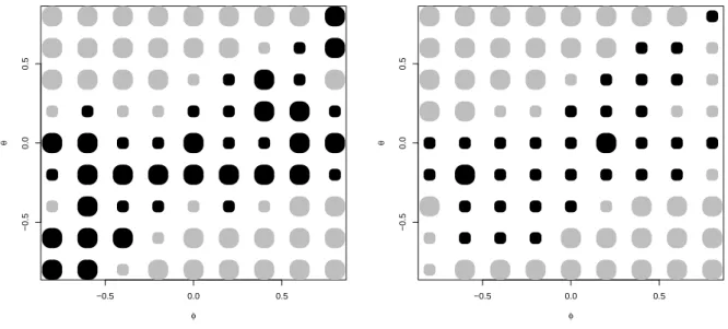
The so-called Greenland graphs, such as those in Figure 1, permit to make this statement more precise. On a sizable portion of the admissible parameter space, AR(1) defeats ARMA(1,1) as a forecasting model, even though θis not exactly zero, i.e. parameter values are outside ΘR. This area—we call it Greenland according to an original color version of the graph—shrinks as the sample size grows. The sizable area of AR dominance is not paralleled by a similar area of MA dominance. The MA(1) model is a comparatively poor forecast tool, and we will exclude it from further simulation experiments. Although some interesting facts about these preference areas can be determined by analytical means (see, e.g., the rule of thumb in Hendry, 1997), for example the poor performance of the MA forecasts is an issue of the algorithm and can be explored by simulation only.
The graph relies on 1000 replications with Gaussian errors. All trajectories were gen- erated with burn-ins of 100 observations. From samples of size N = 50 and N = 100,
forecasts are generated from AR(1), MA(1), and ARMA(1,1) models with estimated pa- rameters, and the squared prediction error for X51 and, respectively,X101 is evaluated. We generated similar graphs for smaller and slightly larger sample sizes. We certainly do not claim that we are the first to run such simulations, but the graphs serve as a valuable ref- erence for the remainder of the paper and there does not seem to exist an easily accessible source for comparable graphs in the literature. It is obvious that some smoothing or higher numbers of replications will produce clear shapes of the preference areas. We feel, however, that its ragged appearance conveys a good impression of areas where preference for any of the three models is not very pronounced.
−1.0 −0.5 0.0 0.5 1.0
−1.0−0.50.00.51.0
−1.0 −0.5 0.0 0.5 1.0
−1.0−0.50.00.51.0
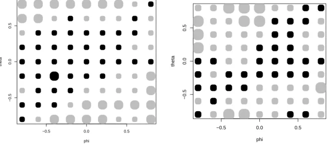
Figure 1: Forecasting data generated by ARMA models with autoregressive coefficient ϕ on the x–axis and moving-average coefficient θ on the y–axis. N = 50 (left) and N = 100 (right).
Comparison of MSE according to AR, ARMA, and MA models with estimated coefficients. Black area has lowest MSE for AR models, gray area for ARMA, and light gray area for MA models.
For empirical work, the applicability of Figure 1 is limited, as it shows the optimal selection of prediction models for given and true parameter values. For a hypothetical researcher who observes ARMA(1,1) data, this decision is not available. If the true values were known, it would be optimal to use them in forecasting. On the other hand, it is not generally possible to draw a comparable figure that has on its axes values of estimates ( ˆϕ,θ) that are available to the hypothetical observer. This would require convening a priorˆ
distribution on the parameter space, thus adopting a Bayesian framework.
For our simulation study, however, these graphs are important benchmarks, as the almost ideal selection procedure between AR(1) and ARMA(1,1) would select AR(1) on the dark area and ARMA(1,1) on the remainder. An ideal procedure may be able to beat this benchmark by varying the classification of specific trajectories over the two regions, but it is unlikely that such improvements are practically relevant. We note explicitly that preferring AR(1) on ΘR only does not lead to optimal forecasting decisions, in contrast to the underlying statistical hypothesis testing problem.
In all our experiments the outcome may depend critically on the estimation procedure used for AR as well as for ARMA models. Generally, we use the estimation routines implemented in R. We feel that the possible dependence of our results on the specific estimation routine need not be seen as a drawback, as we are interested in the typical situation of a forecaster who considers given samples and popular estimation options. In other words, even if other estimation routines perform much better, the R routines are more likely to be relevant as forecasters may tend to use them or similar algorithms.
In detail, we consider the following five strategies and report on pairwise comparisons between them:
1. Training-sample evaluation (TS) over 50% of the available time range. The model with the smaller MSE over the training sample is chosen as the forecasting model;
2. Training-sample evaluation (TS-DM-N) as in # 1, but followed by a Diebold-Mariano (DM) test. The more complex (here, the ARMA) model is only chosen if the DM test statistic is significant at a nominal N(0,1) 5% level;
3. Training-sample evaluation (TS-DM-B) as in # 2, but the significance of the DM statistic is evaluated against a carefully bootstrapped value;
4. Training-sample evaluation (TS-F-B) followed by an F–test evaluation according to Clark and McCracken (2001,2005). This statistic does not follow any standard dis- tribution even in simple cases, so this strategy is evaluated with bootstrapping only;
5. AIC evaluation over the full available sample and choosing the model with the lower AIC value;
6. Training-sample evaluation followed by an evaluation of the concomitant GW statistic over moving windows (TS-GW). The more complex model is chosen only if the GW test statistic is significant at a nominal 5% significance level.
Other predictive accuracy tests can be considered, but choosing these as alternative selection strategies is hardly likely to affect our results. For example, Clark and McCracken (2005) show that in nested applications encompassing tests following Harvey et al. (1998) and DM tests are asymptotically equivalent, and the discriminatory power of their F tests is also close to the other tests, as all of them process the same information.
Basically, all our simulations follow the same pattern with expanding windows. For N = 100, observations t= 52, . . . ,99 are used as a test sample in the sense that models are estimated from training samples t= 1, . . . , T and the mean squared error of one-step out- of-sample forecasts for observations XT+1 is evaluated by averaging over T = 51, . . . ,98.
In the pure TS strategy, the model with the smaller average MSE is selected as the one whose out-of-sample forecast for the observation atN based on the sample t= 1, . . . , N−1 is considered. In the DM strategy, the more complex ARMA model is selected only if the DM test rejects. Otherwise, the DM strategy chooses the simpler AR(1) model to forecast the observation at N.
3.2 The bootstrapped DM test and training
Inoue and Kilian (2006) established the result that, roughly, TS works like an information criterion asymptotically. Depending on whether the share of the training sample in the available sample converges to unity or not, the information criterion can be a consistent one like the BIC by Schwarz or a prediction-optimizing efficient one like the AIC by Akaike.
In small samples, it is now widely recognized that the AIC tends to be too ‘liberal’ in the sense that it leans toward over-parameterization (see McQuarrie and Tsai, 1998), which issue will be evaluated in the next subsection. Thus, the strategy not to accept the more general ARMA(1,1) model as a prediction model unless the DM test additionally rejects its null may benefit prediction.
The TS strategy has been considered, for example, by Inoue and Kilian (2006), who were interested in the question whether it be outperformed by BIC selection. There are
arguments in favor of both TS and BIC. BIC uses the whole sample, while TS restricts attention to the portion that is used for the training evaluation. On the other hand, the property of BIC consistency is asymptotic and need not imply optimality in a small sample. Inoue and Kilian find that BIC dominates TS over large portions of the admissible parameter space. We note that their simulations differ from ours by the non-nested nature of decisions on single realizations: some trajectories may be classified as ARMA by one strategy but as AR by the other, while other trajectories experience the reverse discrepancy.
We do not consider BIC selection in our experiments.
It is well known that the normal significance points of the DM test are invalid if nested models are compared (see Clark and McCracken, 2001, 2012). For our experiment, we obtained correct critical values using the bootstrap-in-bootstrap procedure suggested by Kilian (1998). The known estimation bias for AR models is bootstrapped out in a first run, and another bootstrap with reduced bias is then conducted to deliver significance points. Unfortunately, the bootstrap is time-consuming, thus only 100 bootstrap iterations can be performed for this experiment. Nonetheless, correspondence to the targeted size of 5% is satisfactory.
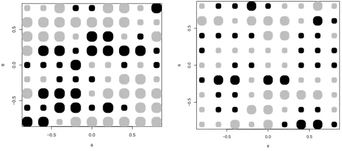
The left graph in Figure 2 shows the result of our Monte Carlo atN = 50. It corresponds to expectations at least with regard to the behavior around the horizontal axis, where the AR model is true. Here, DM testing changes the implicit significance level of the TS procedure of around 20% to 5%. Less AR trajectories are classified incorrectly as ARMA, and forecasting precision improves. At some distance from the axis, TS dominates due to its larger implicit ‘power’ that attains 100% at θ = 0.8. In the graph, the size of the filled circles is used to indicate the intensity of the discrepancy in mean-squared errors. The maximum tilt in favor of DM testing is achieved at (ϕ, θ) = (−0.4,−0.2), the maximum in favor of pure TS occurs along the margins of the square, for extreme values of ϕ and of θ.
An unexpected feature of Figure 2 is the asymmetry of the preference areas: the north- west area with negativeϕ and negative correlation among residuals after a preliminary AR fit appears to be more promising for the DM test than the southeast area with positive ϕ and negative residual correlation after AR fitting. This effect is not easily explained. The Greenland graph at N = 50 is approximately symmetric. Support for the pure AR model
−0.5 0.0 0.5
−0.50.00.5
phi
theta
−0.5 0.0 0.5
−0.50.00.5
phi
theta
Figure 2: AR/ARMA model selected by MSE miminization over a training sample (TS) versus selection based on a Diebold-Mariano test (TS-DM-B) with bootstrapped significance points. Left graph for N = 50, right graph for N = 100. Gray dots express a preference for TS, black dots one for DM. 1000 replications.
is slightly stronger in the northwest than in the southeast, according to TS and to DM, with a difference of around 10 percentage points.
The right graph of Figure 2 shows the results for N = 100. For most parts of the scheme, the version without DM appears to be the preferred strategy. DM dominance has receded to an area approximately matching ΘR, with even two perverse spots along the x–axis. Like the isolated area in the southeast at (0.4,−0.8) and (0.6,−0.8), we interpret them as artifacts. In these areas, the difference in performance between TS and DM is so small that a larger number of replications would be required to bring them out clearly.
We also ran some unreported exploratory experiments with larger N. The preference area for DM versus TS shrinks faster than Greenland as the sample size increases. The DM test yields a reliable decision procedure for AR within ARMA for those who are interested in theoretical data-generating processes, but it does not help in selecting prediction models.
In summary, a tendency is palpable that for even largerN any support for the DM version tends to disappear. The change from an implicit 15-20% test to a 5% test does not benefit forecasting properties.
Generally, we note some typical features of our graphical visualization of the simulations.
A conservative procedure, i.e. one that tends to stay with the simpler AR model, will dominate on the dark area in the Greenland plot, as there it is beneficial to use the AR model as a forecasting tool. A rather liberal procedure, i.e. one that tends to prefer the ARMA model and has ‘high power’ in the traditional sense of hypothesis testing, will dominate on the outer light area of the Greenland plot. In this interpretation, a strategy that dominates on the outer area and on a portion of the inner area can be seen as liberal and relatively promising, while a strategy that inhabits a narrow outer margin is too liberal, and one that lives on a narrow band around ΘR is too conservative to be efficient.
3.3 The bootstrapped F test and training
If a parallel experiment to the previous one is run on the basis of the F test due to Clark and McCracken (2001,2005) that replaces the DM statistic by
N 2 ×
∑N−1
t=N/2(e21,t−e22,t)
∑N−1
t=N/2e22,t ,
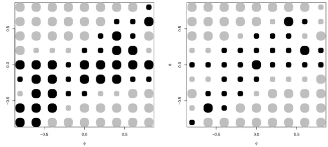
with prediction errors from the two models ej,t, j = 1,2, this yields the outcome shown in Figure 3. For N = 50, the additional testing step boosts forecasting accuracy on ΘR and in some areas that may be artifacts. For N = 100, the procedures with and without the testing step become so close that the picture fades. In summary, the additional testing step helps in small samples if the generating model is AR(1) or at least very close to AR(1), which is not surprising, whereas it does not help at all in larger samples.
−0.5 0.0 0.5
−0.50.00.5
φ
θ
−0.5 0.0 0.5
−0.50.00.5
φ
θ
Figure 3: AR/ARMA model selected by MSE minimization over a training sample (TS) versus selection based on an F test (TS-F-B) with bootstrapped significance points. Left graph for N = 50, right graph for N = 100. Gray dots express a preference for TS, black dots one for the F test. 1000 replications.
3.4 Nested models and naive normal distribution
As we mentioned above, the (normal) DM test is known to suffer from severe distortions in nested model situations, see Clark and McCracken (2001, 2012). Nevertheless, it has been used repeatedly in the empirical forecasting literature, and the typical handling of stochastic properties may be somewhere in between the correct bootstrap used in the previous subsection and the naive N(0,1) distribution suggested in the original DM paper.
Again, we simulate ARMA(1,1) series of length N = 50,100, with Gaussian N(0,1) noise (εt) and the identical design as above. Out-of-sample forecasts for the latter half of the sample are generated on the basis of AR(1) and ARMA(1,1) models with estimated parameters, and the model with the lower MSE is used to predict the observation at position N + 1. Significance of the DM test statistic, however, is now checked against the theoretically incorrect N(0,1) distribution instead of the carefully bootstrapped correct null distribution.
The relative performance of the pure TS strategy and of the DM–test strategy is eval- uated graphically in Figure 4. The area of preference for the DM strategy appears to be a subset of the inner Greenland area, which implies that the selection strategy based on the DM test with normal quantiles is suboptimal.
−0.5 0.0 0.5
−0.50.00.5
φ
θ
−0.5 0.0 0.5
−0.50.00.5
φ
θ
Figure 4: AR/ARMA model selected by MSE minimization over a training sample (TS) versus selection based on a Diebold-Mariano test (TS-DM-N) with ‘naive’ 5%N(0,1) significance points.
Left graph for N = 50, right graph for N = 100. Gray dots express a preference for TS, black dots one for DM. 1000 replications.
3.5 AIC and training
According to Inoue and Kilian (2006), TS and AIC will be equivalent in large samples if the training sample grows linearly with the sample size. In our experiments, we set the training sample at 50% of the complete sample, i.e. slightly more than economic forecasters tend to use although less than would be suggested by an asymptotic approximation to BIC.
The arguments considered by Inoue and Kilian (2006) again apply here. Information criteria tend to exploit the information in the entire sample, while TS concentrates on the part that is used as a training sample. As GW argue, this latter property constitutes an advantage if the generating mechanism changes slowly over time, but our generating models are exclusively time-homogeneous. Rather, TS focuses on the specific aim of the forecasting exercise, while AIC has been derived on grounds of asymptotic properties and is known to perform poorly in small samples (see McQuarrie and Tsai, 1998).
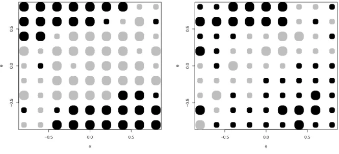
Figure 5 shows the regions where TS and AIC dominate. Among the strategies, AIC is the exception, as it is the only procedure that tends to be more liberal than TS. For this reason, the colors are turned on their heads, and TS dominates around ΘR, whereas AIC dominates in the corners, where it classifies considerably more trajectories into the ARMA(1,1) class. For the larger samples N = 100, AIC gains ground, maybe due to its more efficient processing of the sample information. For the smaller samples N = 50, TS dominance around ΘR is quite pronounced. On the whole, AIC–based forecast model selection evolves as the most serious rival strategy to pure TS.
3.6 Giacomini-White and training
GW considered forecasts based on moving windows of fixed sizem. In a sample of sizeN, N−m−2 such one-step forecasts are available, if the last observationXN is to be reserved for a final evaluation. GW call their test statistic ‘Wald-type’ and define it formally as
Tm,n =n [
n−1
N∑−2 t=m
ht{g(e1,t+1)−g(e2,t+1)} ]′
Ωˆ−n1 [
n−1
N∑−2 t=m
ht{(g(e1,t+1)−g(e2,t+1)} ]
,
withn =N−m−2 andg(x) =x2 in our case andhta 2–vector of ‘test functions’, typically specified as a constant 1 in the first position and the lagged discrepancy g(e1,t)−g(e2,t)
−0.5 0.0 0.5
−0.50.00.5
φ
θ
−0.5 0.0 0.5
−0.50.00.5
φ
θ
Figure 5: Smaller MSE if either TS or AIC are used to select between ARMA(1,1) and AR(1) as prediction models. Left graph for N = 50, right graph for N = 100. Light spots prefer TS, dark spots prefer AIC.
in its second position. Denoting the summand terms by Zm,t+1, the 2×2–matrix ˆΩn is defined as
Ωˆn=n−1
N∑−2 t=m
Zm,t+1Zm,t+1′ .
GW show that under their null this statistic Tm,n will be distributed as χ22. We note that the construction of this test statistic is not symmetric, and we typically are interested in the alternative of method 2 outperforming method 1, such that the discrepancies tend to be positive.
We consider the efficiency of this test as a simplicity booster in the following sense. The AR(1) and the ARMA(1,1) forecast are evaluated comparatively on expanding subsamples as before. If the AR(1) forecast wins, it is selected. If the ARMA(1,1) forecast wins, it is selected only in those cases where the GW test rejects at 5%. In line with the simulations presented by GW, we specify m=N/3 for the window width.
Figure 6 shows that advantages for the GW step are restricted to the Greenland area at N = 50 and weaken for N = 100. It may be argued that running the GW test at risk
−0.5 0.0 0.5
−0.50.00.5
φ
θ
−0.5 0.0 0.5
−0.50.00.5
φ
θ
Figure 6: Smaller MSE if either pure TS or TS jointly with the Giacomini-White test at 5% are used to select between ARMA(1,1) and AR(1) as prediction models. Left graph forN = 50, right graph for N = 100. Light spots prefer pure TS, dark spots prefer TS with GW.
levels around 50% may benefit forecasting. We would like, however, to keep to the way that the procedures are used in current practice, and a conventional risk level is part of the TS-GW procedure in our design.
3.7 Summary of the nested experiment
Overall, it appears that the pure TS strategy that decides on the model to be eventually used for prediction on the basis of a straightforward training-sample evaluation is hard to beat. Any significance test decision on top of it in the sense of simplicity boosting tends to worsen the results over a sizable portion of the parameter space. The least attractive ideas appear to be DM testing based on the incorrect normal distribution and GW. The most competitive idea appears to be the direct usage of information criteria.
In detail, if we compare the MSE values for TS with the bootstrapped DM and for AIC in a graph that is comparable to the hitherto shown figures, no recognizable pattern emerges.
The difference among the two strategies appears to be dominated by the sampling variation
in the Monte Carlo, and the two procedures have comparable quality. TS without any further test does slightly worse but still comes pretty close to the two graphically analyzed strategies. The other suggestions, TS-DM-N and GW, perform considerably worse.
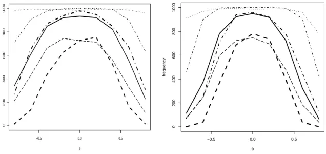
In search of the reasons for the differences in performance among the strategies, one may surmise that these are rooted in the frequency at which either of the two models is selected. Figure 7 shows that this cannot be the complete explanation. For a reasonable visualization, we restrict attention to a vertical slice through our maps, i.e. we show how the strategies behave in the presence of pure MA generating models. For low θ, an AR(1) may be a reasonable approximation for MA(1) behavior, and the implied forecasts may be rather accurate. Thus, TS–based strategies may find it difficult to discriminate among the two models. The primary impression, however, is dominated by a strong three-way classi- fication among strategies: TS and AIC are ‘liberal’ procedures that are locally equivalent to hypothesis tests at significance levels of around 20%; the two test-based strategies with bootstrap approximately match the targeted 5% rate; the naive DM and the GW test are extremely conservative and opt for AR models even in the presence of sizeable MA coef- ficients. Within the three classes, differences are only slight: the F test performs ‘better’
than DM for negative θ and ‘worse’ for θ > 0; AIC appears to dominate TS; and GW is even more conservative than naive DM.
Naive normal DM and Giacomini-White suffer from similar problems. The attempt of the GW test to attain 5% significance at the Greenland boundary instead of the population null hypothesis ΘR implies that the GW–based strategy has a much too strong preference for simplicity. On the other hand, TS and AIC have a comparable tendency toward the more complex model. AIC tends to dominate TS, however, as it selects the better trajectories while the selection frequency is similar. This may be rooted in a more efficient processing of sample information by taking the entire sample into account instead of concentrating on the latter half. Quite successful strategies are TS-DM-B and TS-F. In particular for small parameter values, these strategies boost simplicity efficiently and thus succeed in overcoming the tendency of pure TS to classify trajectories with only weak evidence against AR(1) as ARMA(1,1). Even if the generating models definitely are not AR(1), it remains efficient to see them as AR(1), to estimate just an autoregressive coefficient, and to evaluate
the concomitant forecast. Selection based on the bootstrapped tests and on AIC dominates, and, as AIC is much faster and easier to calculate, the bottom line may be some preference for traditional AIC.
−0.5 0.0 0.5
02004006008001000
θ
frequency
−0.5 0.0 0.5
02004006008001000
θ
frequency
Figure 7: Frequency of choosing the AR(1) model rather than ARMA(1,1) if generating model is MA with given coefficient θ. Curves stand for bootstrapped Diebold-Mariano (bold solid), bootstrapped F (bold dash-dotted), AIC (bold dashed), Giacomini-White (dotted), unconstrained TS (dashed), naive normal Diebold-Mariano (dash-dotted). Left graph for N = 50, right graph forN = 100.
4 Other designs
4.1 A non-nested ARMA design
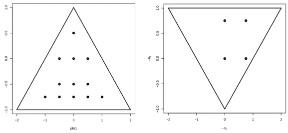
In this experiment, data are generated from ARMA(2,2) processes. There are twelve pairs of AR coefficients. The left graph in Figure 8 shows their distribution across the stability region. Eight pairs yield complex conjugates in the roots of the characteristic AR polyno- mial and hence cyclical behavior in the generated processes. Three pairs imply real roots, and one case is the origin in order to cover pure MA structures. We feel that this design
exhausts the interesting cases in the stability region, avoiding near-nonstationary cases that may impair the estimation step.
These autoregressive designs are combined with the moving-average specifications given in the right graph of Figure 8: a benchmark case without MA component, a first-order MA model, and an MA(2) model with θ1 = 0. Like in our other experiments, errors are generated as Gaussian white noise.
This design is plausible. Second-order models are often considered for economics vari- ables, as they are the simplest linear models that generate cycles. Thus, AR(2) models are not unlikely empirical candidates for data generated from ARMA(2,2): the dependence structure rejects white noise, autoregressive models can be fitted by simple least squares.
Similarly, ARMA(1,1) may be good candidates if a reliable ARMA estimator is available:
often, ARMA models are found to provide a more parsimonious fit than pure autoregres- sions.
−2 −1 0 1 2
−1.0−0.50.00.51.0
phi1
phi2
−2 −1 0 1 2
−1.0−0.50.00.51.0
− θ1
−θ2
Figure 8: Parameter values for the autoregressive part of the generated ARMA models within the triangular region of stable AR models and values for the MA part within the invertibility region for MA(2) models.
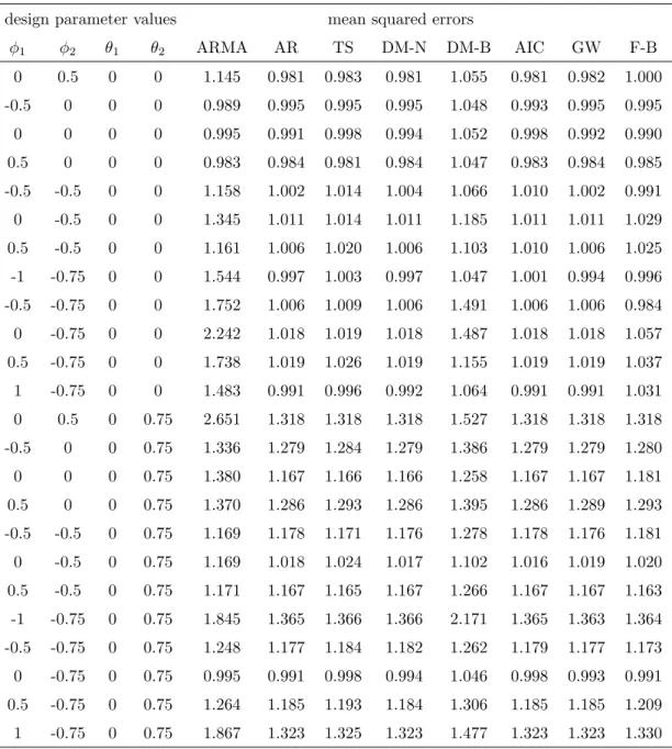
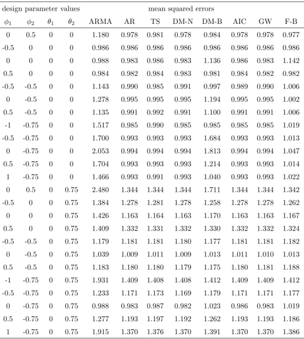
The columns headed ARMA and AR in Tables 1 and 2 show the MSE for predictions using the ARMA(1,1) and the AR(2) models, respectively, if the data-generating process is ARMA(2,2). We note that the prediction models are misspecified for most though not
all parameter values. The first twelve lines correspond to the design (θ1, θ2) = (0,0), when the AR(2) model is correctly specified.
The prevailing impression is that the AR(2) model dominates at most parameter values.
This dominance is partly caused by the comparatively simpler MA part of the generating processes, but it may also indicate greater robustness in the estimation of autoregressive models as compared to mixed models. The relative performance of the two rival models, measured by the ratio of MSE(AR) and MSE(ARMA), remains almost constant as N increases from 100 to 200, which indicates that the large-sample ratios may already have been attained. The absolute performance, however, improves perceptibly as the sample size increases.
The columns headed TS and DM-N report the MSE based on the direct evaluation of a training sample and on the additional DM step on the basis of Gaussian significance points in line with the non-nested design. In pure AR(2) designs, there are mostly gains for imposing the DM step. The null model of the test is the true model, and the extra step helps in supporting it. For strong MA effects, the DM step tends to incur some deterioration.
Another column (DM-B) refers to the DM-based selection using bootstrapped sig- nificance points. This bootstrapped version classifies substantially more trajectories as ARMA(1,1) than DM-N or TS, which incurs a deterioration in performance. Note that bootstrapping has been conducted for the test null model, i.e. the AR(2) model, which is not the data-generating mechanism that is presumed unknown to the forecaster. This situation may be representative for empirical situations where the data-generating mecha- nism is also unknown and the null distribution used for the bootstrap is unreliable. It is of some interest that DM-B does not even perform satisfactorily when AR(2) is the generat- ing model. For most parameter constellations, DM-B performs worst among all competing procedures.
The column AIC selects the forecasting model based on the likelihood, as both rival models have two free parameters. In most cases, AR(2) incurs the better likelihood than ARMA(1,1), the forecasts remain close to the AR forecasts, and AIC wins in approximately one third of all cases, on a par with DM-N and with GW.
Table 1: Results of the simulation for N = 100.
design parameter values mean squared errors
ϕ1 ϕ2 θ1 θ2 ARMA AR TS DM-N DM-B AIC GW F-B
0 0.5 0 0 1.145 0.981 0.983 0.981 1.055 0.981 0.982 1.000 -0.5 0 0 0 0.989 0.995 0.995 0.995 1.048 0.993 0.995 0.995
0 0 0 0 0.995 0.991 0.998 0.994 1.052 0.998 0.992 0.990
0.5 0 0 0 0.983 0.984 0.981 0.984 1.047 0.983 0.984 0.985 -0.5 -0.5 0 0 1.158 1.002 1.014 1.004 1.066 1.010 1.002 0.991 0 -0.5 0 0 1.345 1.011 1.014 1.011 1.185 1.011 1.011 1.029 0.5 -0.5 0 0 1.161 1.006 1.020 1.006 1.103 1.010 1.006 1.025 -1 -0.75 0 0 1.544 0.997 1.003 0.997 1.047 1.001 0.994 0.996 -0.5 -0.75 0 0 1.752 1.006 1.009 1.006 1.491 1.006 1.006 0.984 0 -0.75 0 0 2.242 1.018 1.019 1.018 1.487 1.018 1.018 1.057 0.5 -0.75 0 0 1.738 1.019 1.026 1.019 1.155 1.019 1.019 1.037 1 -0.75 0 0 1.483 0.991 0.996 0.992 1.064 0.991 0.991 1.031 0 0.5 0 0.75 2.651 1.318 1.318 1.318 1.527 1.318 1.318 1.318 -0.5 0 0 0.75 1.336 1.279 1.284 1.279 1.386 1.279 1.279 1.280 0 0 0 0.75 1.380 1.167 1.166 1.166 1.258 1.167 1.167 1.181 0.5 0 0 0.75 1.370 1.286 1.293 1.286 1.395 1.286 1.289 1.293 -0.5 -0.5 0 0.75 1.169 1.178 1.171 1.176 1.278 1.178 1.176 1.181 0 -0.5 0 0.75 1.169 1.018 1.024 1.017 1.102 1.016 1.019 1.020 0.5 -0.5 0 0.75 1.171 1.167 1.165 1.167 1.266 1.167 1.167 1.163 -1 -0.75 0 0.75 1.845 1.365 1.366 1.366 2.171 1.365 1.363 1.364 -0.5 -0.75 0 0.75 1.248 1.177 1.184 1.182 1.262 1.179 1.177 1.173 0 -0.75 0 0.75 0.995 0.991 0.998 0.994 1.046 0.998 0.993 0.991 0.5 -0.75 0 0.75 1.264 1.185 1.193 1.184 1.306 1.185 1.185 1.209 1 -0.75 0 0.75 1.867 1.323 1.325 1.323 1.477 1.323 1.323 1.330
design parameter values mean squared errors
ϕ1 ϕ2 θ1 θ2 ARMA AR TS DM-N DM-B AIC GW F-B
0 0.5 0.75 0 0.980 0.984 0.982 0.985 1.053 0.982 0.984 0.983 -0.5 0 0.75 0 1.010 1.009 1.012 1.006 1.080 1.012 1.016 1.008 0 0 0.75 0 1.006 1.086 1.020 1.063 1.047 1.012 1.083 1.040 0.5 0 0.75 0 0.995 1.147 1.017 1.048 1.092 1.003 1.120 1.039 -0.5 -0.5 0.75 0 1.565 1.212 1.220 1.211 1.410 1.218 1.212 1.234 0 -0.5 0.75 0 1.316 1.304 1.278 1.294 1.337 1.275 1.302 1.316 0.5 -0.5 0.75 0 1.260 1.317 1.281 1.264 1.331 1.297 1.303 1.294 -1 -0.75 0.75 0 1.829 1.270 1.280 1.270 1.389 1.274 1.270 1.271 -0.5 -0.75 0.75 0 2.553 1.360 1.371 1.360 2.189 1.360 1.360 1.370 0 -0.75 0.75 0 2.284 1.436 1.475 1.438 2.019 1.444 1.434 1.704 0.5 -0.75 0.75 0 2.047 1.435 1.496 1.443 2.028 1.450 1.437 1.626 1 -0.75 0.75 0 2.000 1.413 1.441 1.410 1.961 1.425 1.402 1.639 0 0.5 0.75 0.75 1.856 1.635 1.657 1.639 1.758 1.635 1.636 1.653 -0.5 0 0.75 0.75 1.443 1.277 1.283 1.280 1.353 1.277 1.277 1.296 0 0 0.75 0.75 1.300 1.293 1.290 1.294 1.383 1.293 1.292 1.303 0.5 0 0.75 0.75 1.386 1.272 1.281 1.275 1.361 1.272 1.272 1.271 -0.5 -0.5 0.75 0.75 1.067 1.069 1.066 1.068 1.120 1.072 1.069 1.070 0 -0.5 0.75 0.75 1.288 1.179 1.189 1.183 1.264 1.179 1.178 1.214 0.5 -0.5 0.75 0.75 1.618 1.305 1.329 1.306 1.377 1.305 1.310 1.337 -1 -0.75 0.75 0.75 1.051 1.054 1.051 1.053 1.141 1.054 1.054 1.054 -0.5 -0.75 0.75 0.75 1.117 1.067 1.073 1.067 1.123 1.068 1.069 1.067 0 -0.75 0.75 0.75 1.680 1.326 1.353 1.324 1.413 1.327 1.327 1.360 0.5 -0.75 0.75 0.75 2.366 1.515 1.535 1.520 1.826 1.515 1.526 1.836 1 -0.75 0.75 0.75 3.058 1.630 1.636 1.629 2.631 1.630 1.632 1.727
Table 2: Results of the simulation for N = 200.
design parameter values mean squared errors
ϕ1 ϕ2 θ1 θ2 ARMA AR TS DM-N DM-B AIC GW F-B
0 0.5 0 0 1.180 0.978 0.981 0.978 0.984 0.978 0.978 0.977 -0.5 0 0 0 0.986 0.986 0.986 0.986 0.986 0.986 0.986 0.986
0 0 0 0 0.988 0.983 0.986 0.983 1.136 0.986 0.983 1.142
0.5 0 0 0 0.984 0.982 0.984 0.983 0.981 0.984 0.982 0.982 -0.5 -0.5 0 0 1.143 0.990 0.985 0.991 0.997 0.989 0.990 1.006 0 -0.5 0 0 1.278 0.995 0.995 0.995 1.194 0.995 0.995 1.002 0.5 -0.5 0 0 1.135 0.991 0.992 0.991 1.100 0.991 0.991 1.006 -1 -0.75 0 0 1.517 0.985 0.990 0.985 0.985 0.985 0.985 1.019 -0.5 -0.75 0 0 1.700 0.993 0.993 0.993 1.684 0.993 0.993 1.013 0 -0.75 0 0 2.053 0.994 0.994 0.994 1.813 0.994 0.994 1.047 0.5 -0.75 0 0 1.704 0.993 0.993 0.993 1.214 0.993 0.993 1.014 1 -0.75 0 0 1.466 0.993 0.991 0.993 1.040 0.993 0.993 1.022 0 0.5 0 0.75 2.480 1.344 1.344 1.344 1.711 1.344 1.344 1.342 -0.5 0 0 0.75 1.384 1.278 1.281 1.278 1.258 1.278 1.278 1.262 0 0 0 0.75 1.426 1.163 1.164 1.163 1.170 1.163 1.163 1.167 0.5 0 0 0.75 1.409 1.332 1.331 1.332 1.330 1.332 1.332 1.324 -0.5 -0.5 0 0.75 1.179 1.181 1.181 1.180 1.177 1.181 1.181 1.182 0 -0.5 0 0.75 1.039 1.009 1.011 1.009 1.013 1.011 1.010 1.013 0.5 -0.5 0 0.75 1.183 1.180 1.180 1.179 1.175 1.180 1.181 1.188 -1 -0.75 0 0.75 1.931 1.409 1.408 1.408 1.412 1.409 1.409 1.412 -0.5 -0.75 0 0.75 1.233 1.171 1.173 1.169 1.179 1.171 1.171 1.177 0 -0.75 0 0.75 0.988 0.983 0.987 0.982 1.023 0.986 0.983 1.019 0.5 -0.75 0 0.75 1.277 1.193 1.197 1.192 1.262 1.193 1.193 1.186 1 -0.75 0 0.75 1.915 1.370 1.376 1.370 1.391 1.370 1.370 1.386