On the Usefulness of the Diebold-Mariano Test in the Selection of Prediction Models: Some Monte Carlo Evidence

IHS Economics Series Working Paper 276

November 2011

On the Usefulness of the Diebold- Mariano Test in the Selection of Prediction Models: Some Monte Carlo Evidence

Mauro Costantini

Robert M. Kunst

Impressum Author(s):

Mauro Costantini, Robert M. Kunst Title:

On the Usefulness of the Diebold-Mariano Test in the Selection of Prediction Models:

Some Monte Carlo Evidence ISSN: Unspecified

2011 Institut für Höhere Studien - Institute for Advanced Studies (IHS) Josefstädter Straße 39, A-1080 Wien

E-Mail: o ce@ihs.ac.atffi Web: ww w .ihs.ac. a t

All IHS Working Papers are available online: http://irihs. ihs. ac.at/view/ihs_series/

This paper is available for download without charge at:

https://irihs.ihs.ac.at/id/eprint/2097/

On the Usefulness of the Diebold-Mariano Test in the Selection of Prediction Models:

Some Monte Carlo Evidence

Mauro Costantini, Robert M. Kunst

276

Reihe Ökonomie

Economics Series

276 Reihe Ökonomie Economics Series

On the Usefulness of the Diebold-Mariano Test in the Selection of Prediction Models:

Some Monte Carlo Evidence

Mauro Costantini, Robert M. Kunst November 2011

Institut für Höhere Studien (IHS), Wien

Institute for Advanced Studies, Vienna

Contact:

Robert M. Kunst

Department of Economics and Finance Institute for Advanced Studies Stumpergasse 56

1060 Vienna, Austria

: +43/1/599 91-255 email: kunst@ihs.ac.at and

Department of Economics University of Vienna

Mauro Costantini University of Vienna BWZ – Bruenner Str. 72 A-1210 Vienna, Austria

: +43/1/4277-37478

email: mauro.costantini@univie.ac.at

Founded in 1963 by two prominent Austrians living in exile – the sociologist Paul F. Lazarsfeld and the economist Oskar Morgenstern – with the financial support from the Ford Foundation, the Austrian Federal Ministry of Education and the City of Vienna, the Institute for Advanced Studies (IHS) is the first institution for postgraduate education and research in economics and the social sciences in Austria. The Economics Series presents research done at the Department of Economics and Finance and aims to share ―work in progress‖ in a timely way before formal publication. As usual, authors bear full responsibility for the content of their contributions.

Das Institut für Höhere Studien (IHS) wurde im Jahr 1963 von zwei prominenten Exilösterreichern – dem Soziologen Paul F. Lazarsfeld und dem Ökonomen Oskar Morgenstern – mit Hilfe der Ford- Stiftung, des Österreichischen Bundesministeriums für Unterricht und der Stadt Wien gegründet und ist somit die erste nachuniversitäre Lehr- und Forschungsstätte für die Sozial- und Wirtschafts- wissenschaften in Österreich. Die Reihe Ökonomie bietet Einblick in die Forschungsarbeit der Abteilung für Ökonomie und Finanzwirtschaft und verfolgt das Ziel, abteilungsinterne Diskussionsbeiträge einer breiteren fachinternen Öffentlichkeit zugänglich zu machen. Die inhaltliche Verantwortung für die veröffentlichten Beiträge liegt bei den Autoren und Autorinnen.

Abstract

In evaluating prediction models, many researchers flank comparative ex-ante prediction experiments by significance tests on accuracy improvement, such as the Diebold-Mariano test. We argue that basing the choice of prediction models on such significance tests is problematic, as this practice may favor the null model, usually a simple benchmark. We explore the validity of this argument by extensive Monte Carlo simulations with linear (ARMA) and nonlinear (SETAR) generating processes. For many parameter constellations, we find that utilization of additional significance tests in selecting the forecasting model fails to improve predictive accuracy.

Keywords

Forecasting, time series, predictive accuracy, model selection!

JEL Classification

C22, C52, C53

Comments

We thank participants of conferences in Prague, Dublin, Oslo, and Graz, particularly Jan de Gooijer, Neil Ericsson, Werner Mueller, and Helga Wagner, for helpful comments. All errors are ours.

Contents

1 Introduction 1

2 The theoretical background 2

3 The simulations 4

3.1 A nested design ... 4

3.2 A non-nested design ... 8

3.3 A nonlinear generation mechanism ... 12

3.4 A realistic generation mechanism ... 14

4 Summary and conclusion 16

References 18

1 Introduction

In the search for the best forecasting model or procedure for their data, researchers routinely reserve a portion of their samples for out-of-sample prediction experiments.

Instinctively, they feel that a model or procedure that has shown its advantages for a training sample will also be a good choice for predicting the unknown future beyond the end of the available data. Many textbooks on forecasting or econometrics rec- ommend such training-sample comparisons. Following the publication of the seminal work by Diebold and Mariano (1995, DM), it has become customary and often required to add an evaluation of significance to forecast comparisons. This may have led to widespread doubts on the recommendation by the primary comparisons, if differences among rivals cannot be shown to be statistically significant.

Currently, many studies that compare the forecasting accuracy of several pre- diction models or procedures subject their results to a significance test, usually the Diebold-Mariano (DM) test (Diebold and Mariano, 1995) or a variant thereof. It is customary to choose one of the procedures as the ‘simple’ or ‘benchmark’ procedure and to assign significance to the increase in accuracy achieved by a more sophisticated rival. The impression conveyed by this practice is that the sophisticated procedure is recommended only if it is ‘significantly’ better than the benchmark, not just if it has better accuracy statistics. We thus assume that the idea behind the practice of DM testing is that the benchmark is to be preferred unless it is defeated significantly, in the spirit of a model selection procedure. We concede that the motivation for DM testing may be different, for example to simply add to a summary picture, but we feel that our assumed aim is implicitly shared by many researchers in forecasting.

Two main arguments can be raised against this practice. The arguments are connected, although this may not be immediately recognized. First, the null hypoth- esis of the DM test, i.e. the exact equality of population values or expectations of statistics from two comparatively simple forecasting models or other procedures is unlikelya priori. Except in artificial designs, the true data-generating process will be tremendously more complex than both rival prediction models. Classical hypothesis testing, however, requires a plausible null. This can be seen best in a Bayes inter- pretation of classical testing. In significance tests with fixed risk level, the implicit priors given to both hypotheses depend on the sample size. In small samples, the null has a considerable prior probability that gradually shrinks as the sample size grows.

Classical testing with an implausible null, then, implies a sizeable small-sample bias in favor of this null. In the example of concern here, this means that the benchmark model implicitly obtains a strong prior.

The second argument is that the original forecast comparison, assuming it is a true out-of-sample experiment, is a strong model-selection tool on its own grounds.

Depending on specification assumptions, the literature on statistical model selec- tion (Wei, 1992, Inoue and Kilian, 2006, Ing, 2007) has shown that minimizing prediction errors over a training sample that is a part of the observed data can be asymptotically equivalent to traditional information criteria, such as AIC and BIC. Conducting a test ‘on top’ of the information criterion decision, however, is tantamount to increasing the penalty imposed in these criteria and may lead to an

1

unwanted bias in favor of simplicity. Whereas such a bias in favor of simplicity may correspond to the forecaster’s preferences, we note that the same effect can be ob- tained by an information criterion with a stronger penalty without any additional statistical testing. This remark applies more generally to testing ‘on top’ of informa- tion criteria, as it was investigated by Linhart(1988).

Within this paper, we restrict attention to binary comparisons between a compar- atively simple time-series model and a more sophisticated rival. Main features should also be valid for the general case of comparing a larger set of rival models, with one of them chosen as the benchmark. Following some discussion on the background of the problem, we present results of three simulation experiments in order to explore the effects for sample sizes that are typical in econometrics.

The remainder of this paper is organized as follows. Section 2 reviews some of the fundamental theoretical properties of the problem of testing for relative predictive accuracy following a training-set comparison. Section 3 reports three Monte Carlo experiments: one with a nested linear design, one with a non-nested linear design, one with a SETAR design that was suggested in the literature (Tiao and Tsay, 1994) to describe the dynamic behavior of a U.S. output series, and one with a design based on a three-variable vector autoregression that was fitted to macroeconomic U.K. data by Costantini and Kunst(2011). Section 4 concludes.

2 The theoretical background

Typically, the Diebold-Mariano (DM) test and comparable tests are performed on accuracy measures such as MSE (mean squared errors) following an out-of-sample forecasting experiment, in which a portion of size S from a sample of size T is predicted. In a notation close to DM, the null hypothesis of such tests is

Eg(e1) = Eg(e2),

wheree_j, j= 1,2 denote the prediction errors for the two rival forecasts, g(.) is some function—for example, g(x) =x² for the MSE—and E denotes the expectation op- erator. The out-of-sample prediction experiment (SOOS for simulated out-of-sample according to Inoue and Kilian, 2006) is, however, in itself comparable to an in- formation criterion. The asymptotic properties of this SOOS criterion depend on regularity assumptions on the data-generating process, as usual, but critically on the large-sample assumptions onS/T.

IfS/T is assumed to converge to a constant in the open interval (0,1),Inoue and Kilian(2006) show that the implied SOOS criterion is comparable to traditional ‘ef- ficient’ criteria such as AIC. The wording ‘efficient’ is due toTsai and McQuarrie (1998) and relates to the property of optimizing predictive performance at the cost of a slight large-sample inconsistency in the sense that profligate (though valid) models are selected too often asT → ∞.

If S/T is assumed to converge to one, Wei (1992) has shown that the implied SOOS criterion becomes consistent in the sense that it selects the true model, assum- ing such a one exists, with probability one asT → ∞. Note thatWei(1992) assumes

2

that all available observations are predicted, excluding only some few observations at the sample start, where the estimation of a time-series model is not yet possible.

If a consistent model-selection procedure is flanked by a further hypothesis test that has the traditional test-consistency property, in the sense that it achieves its nominal significance level on its null and rejection with probability one on its alter- native, this does not affect the asymptotic property of selection consistency, unless there is a strong and negative dependence between the test statistic and the infor- mation criterion. Whereas, in the issue of concern this dependence is more likely to be positive, we consider briefly the case of independence as a benchmark.

Proposition 1. Suppose there exists a consistent information criterion τ1 and an independent test-consistent significance testτ2 at a given significance levelα2. Then, the joint decision from rejectingH0 if both criteria prefer the alternative is a consis- tent model selection procedure.

This proposition is easily proofed, as the consistent information criterion entails an implicit significance levelα1 that depends onT and approaches 0 asT → ∞(see, e.g.,Camposet al., 2003, for a small-sample evaluation of implicit significance levels for information criteria). If the null model is true, τ1 selects the correct model with probability one in the limit andτ2 with probability 1−α2. Even ifτ2 rejects, τ1 will decide correctly, and its decision dominates for largeT. Conversely, if the alternative model is true, both τ_j forj= 1,2 select the correct alternative asT → ∞.

While this result appears to imply that flanking a consistent criterion with a hypothesis test is innocuous, note that this joint test does not preserve the original significance level. More specifically, we have:

Proposition 2. Suppose there exists an information criterion τ1 with implicit sig- nificance levelα1(T) at T, and an independent test-consistent significance testτ2 at levelα2. Then, the joint test has critical levelα1(T)α2.

This property is obvious but implicit significance levels for customary information criteria are often not readily available. For the inconsistent AIC, the asymptotic implicit significance level is easily demonstrated to be around 0.14. Flanking it with a 5% test implies a level of 0.007. In moderate samples, BIC has a lower implicit level, and the thus implied level for the joint test can be below 0.1%. Thus, even if the asymptotic decision will be correct, the procedure entails a strong preference for the null model that will only be rejected in extreme cases.

Clearly, the DM statistic and a typical consistent information criterion, whether SOOS or BIC, will not be independent, which mitigates this strong a priori null preference. With exact dependence, the implicit levelα1(T) is attained as it is usually lower than the specified level α2. In this case, the DM test decision is ignored. In any other case, the preference for the null will be stronger than that implied by the information criterion. This fact promises a bleak prospect for flanking the IC decision: either flanking is not activated or it generates a bias toward the null. The strength of this bias will be the subject of our simulation experiments.

In particular, we find it useful to study the situation given by the following propo- sition:

3

Proposition 3. Suppose there exists a consistent information criterionτ such that between two modelsM1 andM2 the eventτ >0 indicates a preference forM2, while τ ≤0 prefersM1. Assume the user instead bases her decision onτ > τ0 withτ0 >0.

This decision will be inconsistent in the sense that, as T → ∞, the probability of preferringM1 although M2 is true, will not converge to 0.

This proposition is easily proofed by indirect argument. If the decision were consistent, the cases with τ1 ∈ (0, τ0] would be correctly classified as belonging to M1, while in fact, according to assumptions, they belong to M2.

Depending on the nature of the true data-generation mechanism, particularly on whether the models are nested or not, flanking the consistent SOOS criterion with a DM statistic may lead to situations close to the one being described by Proposition 3.

In typical applications of significance tests, the criterion statistic τ can be properly scaled to (τ −τ0)/f(T), such that it converges to 0 for M1 and to ∞ forM2. Then, it will not hit a non-zero interval (0, τ0] for largeT, and consistency is unaffected. If the significance level for the DM test, however, is gradually reduced asT → ∞, as it is often recommended in hypothesis testing in order to obtain a fully consistent test, the inconsistency may be relevant. We note once more that the typical empirical situation is one where the data-generating process (DGP) is more complex than the entertained prediction models, and an exact validity of the DM null hypothesis is implausible.

This offers an even bleaker prospect for the practice of testing on top of the training-sample comparison. However, we are less interested here in asymptotic prop- erties than in finite-sample effects. These can only be reliably studied by means of Monte Carlo with realistic assumptions on the DGP and on entertained prediction models. To this aim, we assume in general that the DGP is more complex than the entertained rivals, which is obvious from our second and third simulation designs. For the very first and basic design, we use a typical textbook situation as a benchmark.

3 The simulations

3.1 A nested design

The original DM test is known to suffer from severe distortions for nested model situations, see Clark and McCracken (2001). Nevertheless, it has been used repeatedly by empirical forecasters, and we see this simple nested design as a bench- mark case with some practical relevance.

Our basic design does not allow for mis-specification in the sense that at least one of the forecasting models corresponds to the data-generating process. In particular, we simulate ARMA(1,1) series of lengthN according to

X_t =φX_t−1+ε_t−θε_t−1,

fort= 1, . . . , N, with Gaussian N(0,1) noise (εt). The autoregressive coefficientφ is varied over the set{0,0.3,0.5,0.7}, such that all models are stationary and no model touches upon the sensitive non-stationarity boundary. We also considered φ = 0.9

4

but these simulations suffer from numerical problems, and ARMA estimators often fail to converge.

A burn-in of 100 observations should guarantee that potential dependence on starting values is not a critical issue. We only consider positive φ values, as this corresponds to typical correlation patterns in economic data. The moving-average coefficient θ is varied over the set {−0.9,−0.7,−0.5,−0.3,0,0.3,0.5,0.7,0.9}. 1000 replications of each constellation are generated.

As forecasting models, we consider the autoregressive AR(1) model X_t=φX_t−1+ε_t

and the ARMA(1,1) model. The AR(1) candidate is correctly specified for θ = 0 and for φ = θ. In the latter case, the generated series are white noise. In all other parameter constellations, the AR(1) model is theoretically misspecified. It is to be expected that a reasonable selection procedure chooses the AR(1) on its ‘home ground’

Θ_R={(φ, θ)|θ= 0 orθ=φ},

and the ARMA(1,1) model for stronger deviations from Θ_R. It is also expected that in small samples AR(1) will outperform ARMA(1,1) even for cases outside Θ_R and will be selected accordingly.

Our expectations are met by the simulation results for N = 100. Observations t= 52, . . . ,99 are used as a training sample in the sense that models are estimated from samples t = 1, . . . , T and the mean squared error of one-step out-of-sample forecasts for observations X_T+1 is evaluated by averaging over T = 51, . . . ,98. The AR(1) forecast is clearly superior on Θ_R and appears to dominate for some other cases. In fact, the AR(1) model yields a smaller MSE for two thirds of all replications for (φ, θ) = (0.3,0.5), while this quota falls to 3 out of 1000 for (φ, θ) = (0.3,−0.9).

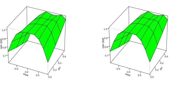
Figure 1 provides a graphical representation of the situation. The simpler AR forecast dominates slightly on the two branches of the set Θ_Rand is markedly worse as the parameter values move away from the set. This picture is surprisingly similar for N = 100 andN = 200, excepting a slight gain for ARMA forecasting in larger samples. While the ‘true’ model should clearly dominate for larger N, the ratios summarize expanding windows over a wider range of N values and thus do not cor- respond to expectations. This situation changes for the second step of the prediction experiment, as observations at positions t= 100 andt= 200 are then evaluated.

A virtual forecaster who is interested in forecasting observation XN may use this comparison to choose the better forecasting model, thus extrapolating the observed relative performance. We were surprised at the quality of this procedure. It appears that even the ‘incorrect’ choice of an AR(1) model at larger distance from ΘR can benefit forecasting accuracy. Some trajectories are infested by short sequences of large errors, for example, which may create poor estimates for the ARMA(1,1) parameters.

The more ‘robust’ AR(1) estimation at t < N often continues its dominance for t=N.

If this procedure is modified by conducting a DM test and sticking to the AR model unless the dominance of the ARMA scheme is significant at 5%, the MSE increases over almost the whole parameter space. Only in some cases with θ = 0

5

theta

−0.5 0.0

0.5

phi

0.0 0.2

0.4 0.6 MSE r

atio

0.7 0.8 0.9 1.0

theta

−0.5 0.0

0.5

phi

0.0 0.2

0.4 0.6 MSE r

atio

0.7 0.8 0.9 1.0

Figure 1:

does the MSE decrease, as the DM test enhances the support for the pure AR model that is beneficial for such values. In other words, the bias in favor of the null has small benefits if the null is true but causes a sizeable deterioration if it is false. Note that even for the high MA values with|θ|= 0.9, an AR model is selected in 20% of the replications.

Figure 2 provides a summary evaluation of the relative frequency for the implied selection of AR and ARMA models. The pure training-set comparison supports AR models over Θ_R and much less so otherwise. For larger N, the selection frequency for pure AR models approaches 0 for large |θ|. The preferences in DM–supported selection are less pronounced, and some AR preference survives atN = 200 even for large |θ|values.

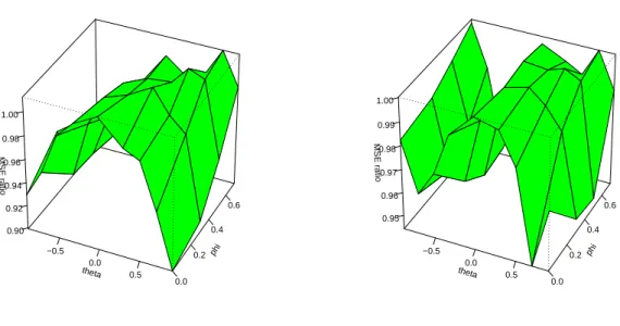
Figure 3 again provides a graphical representation of the situation. With N = 100, the forecast based on the selection dictated by an MSE evaluation over the training sample strictly dominates the forecast that used an additional DM test, excepting a part of the ΘR set. With N = 200, the race between the two selection strategies becomes closer. Particularly for the cases with θ = −0.9 and θ = 0.9, close to non-invertibility, a relative gain for the procedure using the flanking DM test becomes obvious, though even there the procedure without that test still dominates.

Performance becomes trimodal, with near-equivalence between approaches for nearly non-invertible cases and for pure AR models, and more palpable advantages for skipping the DM-test step for intermediate values ofθ.

Generally, dominance or at least equal performance of the DM-guided model selection is mainly restricted to the case θ = 0, i.e. the pure AR model. For most other cases, the additional DM step yields a deterioration in forecasting accuracy.

6

theta

−0.5 0.0

0.5

phi 0.0

0.2 0.4

0.6 frequency

0.2 0.4 0.6

theta

−0.5 0.0

0.5

phi 0.0

0.2 0.4

0.6 frequency

0.0 0.2 0.4 0.6

theta

−0.5 0.0

0.5

phi 0.0

0.2 0.4

0.6 frequency

0.2 0.4 0.6 0.8

theta

−0.5 0.0

0.5

phi 0.0

0.2 0.4

0.6 frequency

−0.2 0.0 0.2 0.4 0.6 0.8

Figure 2:

7

theta

−0.5 0.0

0.5

phi

0.0 0.2

0.4 0.6 MSE r

atio

0.90 0.92 0.94 0.96 0.98 1.00

theta

−0.5 0.0

0.5

phi

0.0 0.2

0.4 0.6 MSE r

atio

0.95 0.96 0.97 0.98 0.99 1.00

Figure 3:

3.2 A non-nested design

In this second experiment, data are generated from ARMA(2,2) processes. There are twelve pairs of AR coefficients. The left graph in Figure 4 shows their distribution across the stability region. Eight pairs yield complex conjugates in the roots of the characteristic AR polynomial and hence cyclical behavior in the generated processes.

Three pairs imply real roots, and one case is the origin to include the case of a pure MA structure. We feel that this design exhausts the interesting cases in the stability region, avoiding near-nonstationary cases that may impair the estimation step.

These autoregressive designs are combined with the moving-average specifications given in the right graph of Figure 4: a benchmark case without MA component, a first-order MA model, and an MA(2) model withθ1 = 0.

This design is not entirely arbitrary. Second-order models are often considered for economics variables, as they are the simplest linear models that generate cycles.

Thus, AR(2) models are not unlikely empirical candidates for data generated from ARMA(2,2): the dependence structure rejects white noise, autoregressive models can be fitted by simple least squares. Similarly, ARMA(1,1) may be good candidates if a reliable ARMA estimator is available: often, ARMA models are found to provide a more parsimonious fit than pure autoregressions.

The columns headed MSE(AR) and MSE(ARMA) in Table 1 and Table 2 show the MSE for predictions using the ARMA(1,1) and the AR(2) models, respectively, if the data-generating process is ARMA(2,2). We note that the prediction models are misspecified for most though not all parameter values. The first twelve lines correspond to the design (θ1, θ2) = (0,0), when the AR(2) model is correctly specified.

8

−2 −1 0 1 2

−1.0−0.50.00.51.0

phi1

phi2

−2 −1 0 1 2

−1.0−0.50.00.51.0

theta1

theta2

Figure 4:

The prevailing impression is that the AR(2) model dominates at most parameter values. This dominance is partly caused by the comparatively simpler MA part of the generating processes, but it may also indicate greater robustness in the estimation of autoregressive models as compared to mixed models. The relative performance of the two rival models, measured by the ratio of MSE(AR) and MSE(ARMA), remains almost constant asNincreases from 100 to 200, which indicates that the large-sample ratios may already have been attained. The absolute performance, however, improves perceptibly as the sample size increases.

By contrast, the columns headed MSE(tr) and MSE(DM) report the comparison between the direct evaluation of a training sample and the additional DM step. For the pure AR(2) model, there are mostly gains for imposing the DM step. The null model of the test is the true model, and the extra step helps in supporting it. For strong MA effects, the DM step tends to incur some deterioration.

In more detail, Tables 1 and 2 show that the DM procedure is beneficial for pre- diction performance in 34 out of 48 designs for N = 100, but that this dominance decreases to 25 cases for N = 200. The training procedure without the DM step wins 10 cases for N = 100 and 12 cases for N = 200, the remaining cases are ties at three digits. A rough explanation is that the AR(2) model usually forecasts bet- ter than the ARMA(1,1) model, often simply due to a better fit to the generating ARMA(2,2) by the asymptotic pseudo-model or due to better estimation properties of the autoregressive estimator, which uses simple and straightforward conditional least squares. The DM step enhances the preference for the AR(2) model and thus im- proves predictive accuracy, though this effect becomes less pronounced as the sample increases. In particular, we note that the procedure without the DM step dominates

9

Table 1: Results of the simulation for

= 100.

φ₁ φ₂ θ₁ θ₂ MSE(ARMA) MSE(AR) MSE(tr) #AR MSE(DM) #AR(DM)

0 0.5 0 0 1.254 1.047 0.983 941 0.981 997

-0.5 0 0 0 1.054 1.044 0.995 529 0.995 893

0 0 0 0 1.053 1.045 0.998 487 0.994 894

0.5 0 0 0 1.047 1.047 0.981 397 0.984 876

-0.5 -0.5 0 0 1.213 1.045 1.014 907 1.004 994

0 -0.5 0 0 1.332 1.045 1.014 962 1.011 1000

0.5 -0.5 0 0 1.191 1.044 1.020 891 1.006 992

-1 -0.75 0 0 1.604 1.045 1.003 979 0.997 999

-0.5 -0.75 0 0 1.767 1.045 1.009 993 1.006 1000

0 -0.75 0 0 2.103 1.045 1.019 997 1.018 1000

0.5 -0.75 0 0 1.730 1.043 1.026 989 1.019 999

1 -0.75 0 0 1.572 1.043 0.996 988 0.992 997

0 0.5 0 0.75 2.651 1.442 1.318 1000 1.318 1000

-0.5 0 0 0.75 1.473 1.392 1.284 827 1.279 987

0 0 0 0.75 1.528 1.260 1.166 983 1.166 999

0.5 0 0 0.75 1.475 1.397 1.293 803 1.286 973

-0.5 -0.5 0 0.75 1.260 1.263 1.171 358 1.176 845

0 -0.5 0 0.75 1.117 1.093 1.024 668 1.017 949

0.5 -0.5 0 0.75 1.257 1.265 1.165 304 1.167 830

-1 -0.75 0 0.75 2.023 1.469 1.366 974 1.366 999

-0.5 -0.75 0 0.75 1.345 1.262 1.184 765 1.182 967

0 -0.75 0 0.75 1.053 1.045 0.998 487 0.994 894

0.5 -0.75 0 0.75 1.341 1.265 1.193 750 1.184 956

1 -0.75 0 0.75 2.001 1.466 1.325 969 1.323 996

0 0.5 0.75 0 1.053 1.050 0.982 458 0.985 881

-0.5 0 0.75 0 1.056 1.070 1.012 389 1.006 835

0 0 0.75 0 1.050 1.146 1.020 164 1.063 626

0.5 0 0.75 0 1.050 1.211 1.017 90 1.048 489

-0.5 -0.5 0.75 0 1.536 1.267 1.220 852 1.211 960

0 -0.5 0.75 0 1.315 1.333 1.278 438 1.294 860

0.5 -0.5 0.75 0 1.311 1.376 1.281 369 1.264 808

-1 -0.75 0.75 0 1.823 1.343 1.280 987 1.270 1000

-0.5 -0.75 0.75 0 2.517 1.422 1.371 995 1.360 1000

0 -0.75 0.75 0 2.136 1.464 1.475 891 1.438 993

0.5 -0.75 0.75 0 2.113 1.486 1.496 875 1.443 989

1 -0.75 0.75 0 2.115 1.518 1.441 849 1.410 987

0 0.5 0.75 0.75 1.932 1.744 1.657 796 1.639 966

-0.5 0 0.75 0.75 1.536 1.350 1.283 890 1.280 992

0 0 0.75 0.75 1.356 1.367 1.290 344 1.294 882

0.5 0 0.75 0.75 1.448 1.345 1.281 854 1.275 992

-0.5 -0.5 0.75 0.75 1.109 1.115 1.066 333 1.068 848

0 -0.5 0.75 0.75 1.315 1.219 1.189 830 1.183 985

0.5 -0.5 0.75 0.75 1.682 1.370 1.329 928 1.306 998

-1 -0.75 0.75 0.75 1.143 1.140 1.051 428 1.053 872

-0.5 -0.75 0.75 0.75 1.137 1.105 1.073 685 1.067 962

0 -0.75 0.75 0.75 1.657 1.365 1.353 884 1.324 991

0.5 -0.75 0.75 0.75 2.413 1.587 1.535 967 1.520 998

1 -0.75 0.75 0.75 3.231 1.758 1.636 983 1.629 999

10

Table 2: Results of the simulation for

= 200.

φ₁ φ₂ θ₁ θ₂ MSE(ARMA) MSE(AR) MSE(tr) #AR MSE(DM) #AR(DM)

0 0.5 0 0 1.246 1.024 0.981 982 0.978 1000

-0.5 0 0 0 1.026 1.024 0.986 495 0.986 909

0 0 0 0 1.027 1.024 0.986 466 0.983 927

0.5 0 0 0 1.024 1.024 0.984 417 0.983 886

-0.5 -0.5 0 0 1.171 1.024 0.985 960 0.991 999

0 -0.5 0 0 1.303 1.024 0.995 997 0.995 1000

0.5 -0.5 0 0 1.164 1.024 0.992 958 0.991 1000

-1 -0.75 0 0 1.535 1.024 0.990 999 0.985 1000

-0.5 -0.75 0 0 1.709 1.024 0.993 1000 0.993 1000

0 -0.75 0 0 2.050 1.024 0.994 1000 0.994 1000

0.5 -0.75 0 0 1.683 1.024 0.993 1000 0.993 1000

1 -0.75 0 0 1.530 1.023 0.991 999 0.993 1000

0 0.5 0 0.75 2.660 1.409 1.344 1000 1.344 1000

-0.5 0 0 0.75 1.450 1.365 1.281 936 1.278 993

0 0 0 0.75 1.508 1.227 1.164 995 1.163 1000

0.5 0 0 0.75 1.453 1.364 1.331 916 1.332 995

-0.5 -0.5 0 0.75 1.231 1.234 1.181 318 1.180 879

0 -0.5 0 0.75 1.094 1.066 1.011 841 1.009 988

0.5 -0.5 0 0.75 1.231 1.235 1.180 311 1.179 866

-1 -0.75 0 0.75 1.957 1.437 1.408 997 1.408 999

-0.5 -0.75 0 0.75 1.310 1.238 1.173 864 1.169 989

0 -0.75 0 0.75 1.027 1.024 0.987 469 0.982 929

0.5 -0.75 0 0.75 1.306 1.238 1.197 848 1.192 984

1 -0.75 0 0.75 1.955 1.440 1.376 995 1.370 1000

0 0.5 0.75 0 1.027 1.027 0.987 478 0.987 916

-0.5 0 0.75 0 1.028 1.048 0.993 278 0.999 797

0 0 0.75 0 1.026 1.122 0.993 68 1.029 484

0.5 0 0.75 0 1.026 1.184 0.986 17 1.040 306

-0.5 -0.5 0.75 0 1.504 1.236 1.233 909 1.219 986

0 -0.5 0.75 0 1.296 1.309 1.266 435 1.290 887

0.5 -0.5 0.75 0 1.284 1.353 1.276 303 1.332 812

-1 -0.75 0.75 0 1.751 1.310 1.309 1000 1.309 1000

-0.5 -0.75 0.75 0 2.444 1.387 1.362 1000 1.362 1000

0 -0.75 0.75 0 2.113 1.440 1.446 966 1.447 1000

0.5 -0.75 0.75 0 2.064 1.461 1.496 950 1.469 999

1 -0.75 0.75 0 2.064 1.481 1.512 942 1.484 998

0 0.5 0.75 0.75 1.918 1.703 1.728 919 1.730 992

-0.5 0 0.75 0.75 1.526 1.317 1.299 961 1.294 999

0 0 0.75 0.75 1.337 1.341 1.320 371 1.318 886

0.5 0 0.75 0.75 1.424 1.322 1.290 967 1.293 1000

-0.5 -0.5 0.75 0.75 1.091 1.096 1.055 306 1.056 841

0 -0.5 0.75 0.75 1.296 1.204 1.179 920 1.177 999

0.5 -0.5 0.75 0.75 1.645 1.348 1.351 986 1.344 1000

-1 -0.75 0.75 0.75 1.114 1.113 1.085 467 1.079 898

-0.5 -0.75 0.75 0.75 1.117 1.090 1.059 756 1.055 988

0 -0.75 0.75 0.75 1.641 1.355 1.352 962 1.349 1000

0.5 -0.75 0.75 0.75 2.344 1.567 1.599 992 1.592 1000

1 -0.75 0.75 0.75 3.140 1.718 1.695 999 1.695 1000

11

the ARMA(2,1) design forN = 200.

3.3 A nonlinear generation mechanism

In this experiment, the data are generated by a nonlinear time-series process that has been suggested byTiao and Tsay(1994) for the growth rate of U.S. gross national product (GNP, an outdated version of the currently used macroeconomic main ag- gregate named gross domestic product). Their self-exciting threshold autoregressive (SETAR) model defines four regimes that correspond to whether an economy is in a recession or an expansion and on whether the recessive or expansive tendencies are accelerating or decelerating.

Define yt as the growth rate of U.S. GNP. The model reads

yt=











−0.015−1.076y_t−1+ε1,t, y_t−1 ≤y_t−2≤0,

−0.006 + 0.630yt−1−0.756yt−2+ε2,t, yt−1 > yt−2, yt−2 ≤0, 0.006 + 0.438y_t−1+ε3,t, y_t−1 ≤y_t−2, y_t−2 >0, 0.004 + 0.443y_t−1+ε4,t, y_t−1 > y_t−2>0.

The standard deviations of the errors σj = q

Eε²_j,t, σ1 = 0.0062, σ2 = 0.0132, σ3 = 0.0094, and σ4 = 0.0082, are an important part of the parametric structure.

In contrast with linear models, threshold models may behave quite differently in qualitative terms if the relative scales of the error processes change.

Even for such a simple nonlinear time-series model class, not all statistical proper- ties are known. Some of them, however, are now fairly well established. For a recent summary of results, see Fan and Yao (2005). Other characteristics are revealed easily by some simulation and inspection.

Within regime 1, which corresponds to a deepening economic recession, the model is ‘locally unstable’, as the coefficient is less than −1. Nevertheless, the model is

‘globally stable’. In fact, it is the large negative coefficient in regime 1, where lagged growth rates are by definition negative, which pushes the economy quickly out of a recession.

The variable tends to remain in regimes 3 and 4 for much longer time spans than in regime 2, and it spends the shortest episodes in the deepening recession of regime 1. Thus, the exercise of fitting linear time-series models to simulated trajectories often leads to coefficient estimates that are close to those for regimes 3 and 4.

For our prediction experiment, we use samples drawn from the SETAR process withN = 100 and N = 200 observations. Burn-in samples of 1000 observations are generated and discarded, as the distribution of the nonlinear generating process may be affected by starting conditions. 1000 replications are performed. The hypothetical forecaster is supposed to be unaware of the nonlinear nature of the DGP, and she fits AR(p) and ARMA(p, p) models to the time series. In analogy to the other experimental designs, the models deliver out-of-sample forecasts for the latter half of the observation range, excepting the very last time point. This latter half is viewed as a training sample. Either the better one of the two models or the one that is

‘significantly’ better according to a DM test, is used to forecast this last time point.

12

Table 3: Results of the SETAR experiment.

MSE

10

frequency

= 100

= 200

= 100

= 200

AR 1.115 1.037 0.518 0.479

ARMA 1.133 1.044 0.482 0.521

50% training

lower MSE 1.113 1.041 0.123 0.118

DM–based 1.112 1.038 0.122 0.106

25% training

lower MSE 1.106 1.042 0.144 0.144

DM–based 1.114 1.035 0.127 0.137

Note: ‘frequency

’ gives the empirical frequency of the model yielding the better predic- tion for the observation at

=

.

We also compare the accuracy of these two strategies with the forecasts that always use the autoregressive or the ARMA model.

A main difference to the other two experiments is that we do not impose a fixed lag orderpon the time-series models. Rather, we determine an optimalpby minimizing AIC over the range 1, . . . , p^∗. The ARMA model uses twice as many parameters as the AR model, so its maximum lag order is set at the popular rule of thumb √

N for the AR and at 0.5√

N for the ARMA model, at least for the smaller samples with n= 50, . . . ,99. For the larger samples, frequent occasions of non-convergence of estimation routines forced us to use 2√

N /3 and √

N /3 instead. This choice is not very influential, as AIC minimization typically implies low lag orders in most replications. p= 1 is the most frequent value.

Table 3 gives the resulting values for the mean squared errors. For 100 observa- tions, the pure AR appears to approximate better than the ARMA model. Choosing the better model on the basis of a pure comparison of performance over the train- ing sample yields an MSE that is comparable to the pure AR model. This average hides some specific features in single replications. For example, the AR model is preferred on the basis of the training sample in 697 out of 1000 replications, while in the remaining 303 cases the ARMA model can be substantially better. Nevertheless, applying the DM test in order to revise the comparison incurs an improvement in accuracy. If preference for ARMA is only accepted if it is ‘significant’, ARMA is selected only in 58 out of 1000 cases. However, in these 58 cases ARMA is slightly better, even for predicting the observation at position 100 that follows the training sample at 50< t ≤99. Again, this evidence is turned on its head once the ARMA model is defined as the simple model and the AR model as the complex one. We opine, however, that this would not be the natural choice.

When the sample size increases to N = 200, the effect in favor of DM testing weakens. Both test-based approaches are beaten by the pure AR model. There

13

is still a slight advantage for the DM–based search. The frequency of significant rejections decreases slightly to 3.5%. Even in these cases do the ARMA models offer no systematic improvement of forecasting accuracy. This result is in keeping with our second experiment, where the beneficial effect of a flanking test weakens in larger samples.

For distributions with high variance, the MSE may not be the most reliable evaluation criterion. When the cases of improvement among the replications are counted, even the slight advantage for test-based selection is turned on its head. At N = 200, in 118 cases is the pure training-sample comparison better, while there are only 106 cases with the opposite ranking. By construction, the forecasts are identical for the remaining 776 cases. At N = 100, wins and losses are fairly identical: the test-based procedure wins 123 times, and the comparison without flanking test 122 times. Application of the DM test helps as much as tossing a coin.

It is interesting that a similar remark holds, however, with respect to the ranking among the AR and ARMA forecasts. For N = 200, the ARMA model forecasts better in 521 out of 1000 cases, even though it yields the larger MSE. Note that the strong preference for the AR model by the training samples is based on an MSE comparison. Counting cases would yield a different selection. With the smaller sample of N = 100, support for the AR model is more unanimous. It yields the smaller MSE as well as the better head count, though with a comparatively small preponderance of 518 cases.

Particularly in this experiment, we also considered different specifications for the relative length of the training set. The empirical literature often uses shorter training sets, and we accordingly reduced them from 50% to 25% of the data. For N = 100, this indeed induces a slight improvement in predictive accuracy, with a stronger effect on the method without additional DM test. For N = 200, this variant entails no change in MSE. Again, selection without DM testing wins with regard to the count of cases. These rather ambiguous effects of shortening the training sample are a bit surprising, as the simulation design involves switches among regimes with locally linear behavior, such that a shorter training set increases the chance that the whole set remains within a regime, which may benefit prediction. Our general impression is that there is little motivation for working with short training sets. This impression is confirmed by some unreported simulation variants for the other two experimental designs.

Similarly, we also considered changing the significance level for the DM test to 10%. This implies that more cases of improved MSE become significant. Indeed, this helps in improving average MSE forN = 100, while there is no change for N = 200 relative to the 5% procedure.

3.4 A realistic generation mechanism

Our main ARMA experiment II is realistic in the sense that it uses prediction models that are simpler than the generation mechanism. It is not realistic in the sense that lag orders of the fitted models are fixed. Typical forecaster may select lag orders via information criteria, as we did in experiment III. For this reason, we include a

14

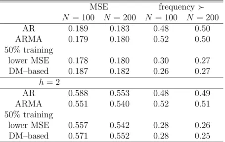
Table 4: Results of the core VAR experiment.

MSE frequency

N

= 100

= 200

= 100

= 200

AR 0.189 0.183 0.48 0.50

ARMA 0.179 0.180 0.52 0.50

50% training

lower MSE 0.178 0.180 0.30 0.27

DM–based 0.187 0.182 0.26 0.27

h

= 2

AR 0.588 0.553 0.48 0.49

ARMA 0.551 0.540 0.52 0.51

50% training

lower MSE 0.557 0.542 0.28 0.26

DM–based 0.571 0.552 0.28 0.25

Note: ‘frequency

’ gives the empirical frequency of the model yielding the better predic- tion for the observation at

=

.

fourth experiment, where generated data are ARMA and the fitted models are AR and ARMA fitted from information criteria. In order to attain a good representa- tiveness of economic data, we adopt a design from an empirical forecasting project by Costantini and Kunst(2011).

Costantini and Kunst(2011) fit vector autoregressions (VAR) to three-variable macroeconomic core sets for the French and U.K. economies. VAR models typically imply univariate ARMA models on their components (e.g., see Lutkepohl, 2005).

From their sets, we select the British VAR as a generating mechanism and focus on the rate of price inflation among its components. Our choice has been guided by the dynamic dependence structures of the components, which turned out to be strongest and thus most interesting for the inflation series.

Table 4 shows that the ARMA forecasts are better than the AR forecasts at both N = 100 and N = 200. We note that the ARMA forecasts are not necessarily based on the true model, as the AIC lag selection tends to find lower orders than the theoretically correct ARMA model class. If the pure training sample is used, the ARMA model is usually preferred, so performance of forecasts based on this selection correspond roughly to the ARMA forecast. If the DM test is used, only around a third of the ‘rejections’ of the AR model are deemed significant at N = 100, and around half of the ‘rejections’ for N = 200. In consequence, the DM-based predictions often correspond to the AR forecasts, which on average leads to a deterioration of performance.

It is perhaps surprising that the dominance of the pure training-sample evaluation is not more pronounced for the larger sample size. One reason is that the generating ARMA model is close to the stability boundary, which often entails unstable estimates for the generated samples that in turn entailed convergence problems with likelihood-

15

based algorithms. For this reason, we switched to a less efficient least-squares ARMA estimate for N = 200. In practice, more accurate estimates may be obtained, which would increase the dominance of the forecasts without the additional DM step. At larger samples, good ARMA estimates should converge to the true generating design, while AR models can only fit approximations at increasing lag length. Just as in the other simulations, our interest mainly focuses on finite-sample performance, not on asymptotic properties.

The lower part of Table 4 provides a parallel evaluation for forecast errors at the larger step size h = 2. All procedures work in an analogous way, with the better model selected if it provides smaller two-step errors etc. Our general impression is that, at larger step sizes, effects point in the same direction but become slightly bit more pronounced. Similar patterns are obtained if larger step sizes are implemented in the other experiments. We do not report detailed results here.

4 Summary and conclusion

It has become customary to subject comparisons of predictive accuracy to an addi- tional step of significance testing, reflecting an unease toward small gains in predictive accuracy achieved by complex prediction models. To this aim, the most widespread test is the DM test due toDiebold and Mariano(1995), whose asymptotic prop- erties can be shown to hold for quite general situations, although they are invalid in comparisons of nested models.

We argue that the potentially implied model selection, i.e. choosing the more complex model only in cases where its benefits are statistically significant, may incur the danger of a bias toward the simple benchmark model. This caveat is based on two established facts: first, the original out-of-sample comparison corresponds to a valid model selection procedure already; second, the null hypothesis tested by the DM test is a priori unlikely to hold exactly in a typical empirical situation.

In order to gain insight into the relevance of our point, we report several Monte Carlo simulations for sample sizes of relevance in economics: N = 100 and N = 200.

In a first simulation with a nested linear design, the additional DM step incurs a general deterioration of the selected model. The selected model after the DM step performs worse than the selected model without the DM step.

In a second situation with a non-nested design that conforms to the assumptions of the DM test, the additional test serves as a ‘simplicity booster’ for the smaller sample ofN = 100 and often leads to gains in predictive accuracy. This effect, which weakens for larger samples, indicates that the simple out-of-sample comparison often achieves its valuable properties for larger samples only. Model selection by usual asymptotic information criteria is known to perform poorly in small samples (see MacQuarrie and Tsai, 1998, among others), and the finite-sample correction of criteria like AICcand AICumay be approximated by an analogous stronger preference for the null expressed by the additional testing step.

In a third design, we adopt a nonlinear time-series process from the literature as the DGP, and we assume that the forecaster entertains linear specifications. While the differences among procedures are small for this design, our general impression is

16

that the additional DM step is of little use here. The training-sample comparison implies a forecasting performance comparable to the better-fitting specification, and the additional DM step hardly changes this performance.

In a fourth design, we use a VAR with coefficients fitted to macroeconomic data for the United Kingdom and we focus on predicting the component with the strongest time dependence structure, the rate of inflation. In a VAR(2), components follow

‘marginal’ univariate ARMA models, so the design resembles the second experiment.

However, in this experiment we entertained AR and ARMA prediction models guided by an AIC search. Then, the DM step implies a deterioration of prediction accuracy in all considered variants, including increased prediction horizons.

Our general impression from the prediction experiments is that adding a signif- icance test to a selection of prediction models guided by a training sample fails to systematically improve predictive accuracy. The evaluation of prediction accuracy of rival models over a substantial part of the available sample is a strong selection tool in itself that hardly needs another significance test to additionally support the simpler model.

Acknowledgements

We thank participants of conferences in Prague, Dublin, Oslo, and Graz, particu- larly Jan de Gooijer, Neil Ericsson, Werner Mueller, and Helga Wagner, for helpful comments. All errors are ours.

17

References

Campos, J., D.F. Hendry, and H.M. Krolzig(2003) ‘Consistent Model Selection by an Automatic Gets Approach,’ Oxford Bulletin of Economics and Statistics 65, 803–819.

Clark, T.E., and M.W.McCracken(2001) ‘Tests of equal forecast accuracy and encompassing for nested models,’Journal of Econometrics 105, 85–110.

Costantini, M., and R.M. Kunst (2011) ‘Combining forecasts based on multiple encompassing tests in a macroeconomic core system,’Journal of Forecasting30, 579–

596.

Diebold, F.X., and R.S.Mariano(1995) ‘Comparing Predictive Accuracy,’Journal of Business and Economic Statistics 13, 253–263.

Fan, J., and Q.Yao (2005)Nonlinear Time Series, Springer.

Ing, C.K. (2007) ‘Accumulated prediction errors, information criteria and optimal forecasting for autoregressive time series,’Annals of Statistics 35, 1238–1277.

Linhart, H. (1988) ‘A test whether two AIC’s differ significantly,’ South African Statistical Journal 22, 153–161.

Lutkepohl, H. (2005) New introduction to multiple time series analysis, Springer- Verlag.

Inoue, A., and L. Kilian (2006) ‘On the selection of forecasting models,’ Journal of Econometrics 130, 273–306.

McQuarrie, A.D.R., and C.-L. Tsai (1998) Regression and Time Series Model Selection, World Scientific.

Tiao, G.C., and R.S. Tsay (1994) ‘Some Advances in Non Linear and Adaptive Modelling in Time Series,’ Journal of Forecasting 13, 109–131.

Wei, C.Z. (1992) ‘On predictive least squares principles,’ Annals of Statistics 20, 1–42.

18

Authors: Mauro Costantini, Robert M. Kunst

Title: On the Usefulness of the Diebold-Mariano Test in the Selection of Prediction Models:

Some Monte Carlo Evidence

Reihe Ökonomie / Economics Series 276

Editor: Robert M. Kunst (Econometrics)

Associate Editors: Walter Fisher (Macroeconomics), Klaus Ritzberger (Microeconomics)

ISSN: 1605-7996

© 2011 by the Department of Economics and Finance, Institute for Advanced Studies (IHS),

Stumpergasse 56, A-1060 Vienna   +43 1 59991-0  Fax +43 1 59991-555  http://www.ihs.ac.at

ISSN: 1605-7996