JournalofGeophysicalResearch:Oceans PUBLICATIONS

(1)

RESEARCH ARTICLE

10.1002/2016JC012238

Nitrous oxide during the onset of the Atlantic cold tongue

D. L. Arevalo-Martınez¹, A. Kock¹, T. Steinhoff¹, P. Brandt², M. Dengler², T. Fischer², A. K€ortzinger¹, and H. W. Bange¹

1Chemical Oceanography Department, Helmholtz Centre for Ocean Research, Kiel, Germany,²Physical Oceanography Department, Helmholtz Centre for Ocean Research, Kiel, Germany

Abstract

The tropical Atlantic exerts a major influence in climate variability through strong air-sea interactions. Within this region, the eastern side of the equatorial band is characterized by strong seasonality, whereby the most prominent feature is the annual development of the Atlantic cold tongue (ACT). This band of low sea surface temperatures (22–238C) is typically associated with upwelling-driven enhancement of surface nutrient concentrations and primary production. Based on a detailed investigation of the distribution and sea-to-air fluxes of N2O in the eastern equatorial Atlantic (EEA), we show that the onset and seasonal development of the ACT can be clearly observed in surface N2O concentrations, which increase progressively as the cooling in the equatorial region proceeds during spring-summer. We observed a strong influence of the surface currents of the EEA on the N2O distribution, which allowed identifying ‘‘high’’ and

‘‘low’’ concentration regimes that were, in turn, spatially delimited by the extent of the warm eastward- flowing North Equatorial Countercurrent and the cold westward-flowing South Equatorial Current. Estimat- ed sea-to-air fluxes of N2O from the ACT (mean 5.1862.59lmol m²²d²¹) suggest that in May–July 2011 this cold-water band doubled the N2O efflux to the atmosphere with respect to the adjacent regions, highlighting its relevance for marine tropical emissions of N2O.

1. Introduction

Nitrous oxide (N2O) is a potent, well-mixed greenhouse gas (GHG) whose atmospheric concentrations have been increasing during the Anthropocene, contributing significantly to the rise in global average temperatures [Bindoff et al., 2013;Hartmann et al., 2013] and stratospheric ozone depletion [Ravishankara et al., 2009]. Since the ocean contributes about one third of the total natural source of N2O to the atmosphere [Ciais et al., 2013] , the assessment of marine emissions of N2O is crucial for improving global atmospheric N2O budget calculations. The tropical Atlantic Ocean exerts a major influence in climate variability through strong ocean-atmosphere interactions, which alter regional temperatures and rainfall patterns on different time scales [Carton et al., 1996;Xie and Carton, 2004;Chang et al., 2006;Brandt et al., 2011;Caniaux et al., 2011;Tokinaga and Xie, 2011]. Within this region, the seasonal variability is particularly accentuated in the eastern equatorial Atlantic (EEA), where pronounced sea surface temperature (SST) and wind speed variations can be observed during the year, mostly in association with the meridional displacement of the inter- tropical convergence zone (ITCZ) [Xie and Carton, 2004]. Thus, in a typical seasonal cycle in the EEA high SST, precipitation and strong stratification can be observed from boreal autumn to early spring, when the southeasterly (SE) trade winds are the weakest and the ITCZ is centered at the Equator. Conversely, during boreal summer, intensified SE trade winds, developing with the northward displacement of the rain band of the ITCZ, trigger the onset of the equatorial Atlantic cold tongue (ACT) due to an associated net shoaling and cooling of the mixed layer [Vinogradov, 1981;Philander and Pacanowski, 1986;Xie and Carton, 2004;

Schlundt et al., 2014].

SST in the ACT can be as low as 22–238C, contrasting with SST as high as 27–298C during the warm season, i.e., boreal autumn to early spring [Caniaux et al., 2011]. The sea surface cooling during the upwelling season in boreal summer is predominantly due to diapycnal downward heat ﬂux [e.g.,Hummels et al., 2013, 2014], which coincides with an upward nutrient ﬂux [Voituriez, 1981], and it is known to be associated with enhanced primary productivity [Christian and Murtugudde, 2003; Grodsky et al., 2008] and emissions of GHGs such as N₂O and CO₂to the atmosphere [Nevison et al., 1995;Takahashi et al., 2009]. Although N₂O

Key Points:

The onset of the Atlantic cold tongue enhances surface concentrations of N2O in the EEA

The regional current system has a major inﬂuence on N2O distribution in the equatorial Atlantic

The equatorial Atlantic acts as a seasonally varying and moderate source of N2O

Supporting Information:

Supporting Information S1

Correspondence to:

D. L. Arevalo-Martınez, darevalo@geomar.de

Citation:

Arevalo-Martınez, D. L., A. Kock, T. Steinhoff, P. Brandt, M. Dengler, T. Fischer, A. K€ortzinger, and H. W. Bange (2017), Nitrous oxide during the onset of the Atlantic cold tongue,J. Geophys. Res. Oceans,122, 171–184, doi:10.1002/2016JC012238.

Received 11 AUG 2016 Accepted 4 NOV 2016

Accepted article online 11 NOV 2016 Published online 13 JAN 2017

VC2016. American Geophysical Union.

Journal of Geophysical Research: Oceans

PUBLICATIONS

(2)

has been measured during several campaigns to the tropical Atlantic over the last decades [Weiss et al., 1992;Oudot et al., 1990, 2002;Walter et al., 2004, 2006], to date no dedicated survey has monitored the seasonal development of the ACT and its effects on the surface distribution and sea-to-air ﬂuxes of this GHG.

Here we present the ﬁrst high-resolution record of surface dissolved and atmospheric N₂O during the onset and progress of the ACT. The ﬁeld work was carried out during two cruises on board of the German research vessel R/V Maria S. Merian (MSM) in May–July 2011, and it was carried out within the framework of the BMBF joint projects NORDATLANTIK and SOPRAN (Surface Ocean Processes in the Anthropocene), as well as the Collaborative Research Center SFB 754.

2. Methods and Data

2.1. Study Area

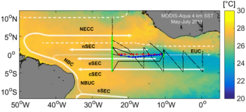
Continuous measurements of N2O were conducted during several along and cross-equatorial sections between 58N–58S and 08W–238W in order to account for the temporal and spatial variability of the region during the onset of the ACT. Figure 1 shows the ship tracks of the MSM 18-2 and 18-3 cruises, as well as the main surface zonal currents crossed during the sampling: The North Equatorial Countercurrent (NECC), and the South Equatorial Current (SEC). The eastward-ﬂowing NECC transports warm, low-salinity waters from the western Atlantic, and reaches its maximal extent in August, coinciding with the northernmost location of the ITCZ [Stramma and Schott, 1999].

Further south, the SEC flows westward carrying waters from the equatorial divergence and western Africa to the northern hemisphere. The northern and central branches of the SEC (nSEC and cSEC, respectively) can be identified in the mean flow field at about 28N and 48S [Brandt et al., 2011], whereas the near-surface westward flow in the equatorial band in between the two mean current cores (the equatorial SEC, eSEC) develops upon strengthening of the equatorial easterlies during boreal summer [Lumpkin and Garzoli, 2005]. Moreover, Figure 1 also shows the Equatorial Undercurrent (EUC) which flows eastward below the near-surface, transporting subtropical saline waters originating in the southern hemisphere and supplying most of the upwelling waters to the ACT region [Hormann and Brandt, 2007;Brandt et al., 2011].

2.2. Underway Measurements

Along-track measurements of dissolved and atmospheric N₂O were performed with an underway system based upon off-axis-integrated cavity output spectroscopy (OA-ICOS) coupled to a shower-type equilibrator, as described byArevalo-Martınez et al. [2013]. Seawater was continuously drawn from about 6.5 m depth either by using the ship’s supply system (centrifugal pump;

MSM 18-2) or a submersible pump (LOWARA, Xylem Inc., Germany) installed at the ship’s moonpool (MSM 18-3), and it was conducted through the equilibration chamber at a rate of 2 L min²¹. Ambient air was sampled by means of an Air Cadet^TM pump (Thermo Fisher Scientiﬁc Inc., Germany) with an inlet located at the ships mast (40 m high). Although ship plumes could potentially contami- nate atmospheric measurements depending on the wind direction, no evidence of such effect was observed after careful examination of our N2O data. In order to

Figure 1.Atlantic cold tongue in 2011. MODIS-Aqua SST in the tropical Atlantic showing the extent of the ACT in May–July 2011. The main zonal surface (solid) and thermocline (dotted) currents during boreal spring/summer are depicted by white arrows: NECC: North Equatorial Countercurrent; nSEC, eSEC, cSEC, and sSEC: northern, equatorial, central, and southern branches of the South Equatorial Current; EUC: Equatorial Undercurrent. The North Brazil Current and Undercurrent (NBC and NBUC, respectively) are also displayed. White dashed lines indicate the approximate extent of the NECC. Black lines indicate the ship tracks of the R/V Maria S. Merian cruises 18-2 (solid) and 18-3 (dashed). CTD stations during the equatorial sections EQ I (20–23 May) and EQ II (8–12 June), as well as the 238W and 108W sections are depicted as red, blue, and green dots/lines, respectively. MODIS-Aqua SST data (monthly means, 4 km resolution) was retrieved from the Goddard Earth Sciences Data and Information Services Center (GES DISC, http://disc.sci.gsfc.nasa.gov/giovanni/), and current bands were drawn based onLumpkin and Garzoli[2005] andBrandt et al. [2011].

(3)

minimize interferences due to water vapor on the sample stream, the air was dried before entering the ana- lyzer by using a cold trap (KWG Isotherm) followed by a Naﬁon^V^R membrane. Control measurements of two reference gases (mixing ratios: 360 and 746 ppb N2O) prepared by Deuste Steininger GmbH (M€uhlhausen, Germany) and calibrated at the Max Planck Institute for Biogeochemistry (Jena, Germany) against the World Meteorological Organization (WMO) standard scale, were used to postcorrect our data for instrumental drift (maximal drift1%) [seeArevalo-Martınez et al., 2013]. Data reduction and calibration procedures were done according toArevalo-Martınez et al. [2013]. N₂O seawater concentrations (C_sw, in nmol L²¹) were computed by means of the expression:

C_sw5b:x⁰:P (1)

wherebis the Bunsen solubility of N2O (in mol L²¹atm²¹) computed at equilibration temperature and in situ salinity with the equation and coefﬁcients ofWeiss and Price[1980],x⁰is the measured dry molar frac- tion of N2O (in nmol mol²¹), andPis the atmospheric pressure (in atm). In order to account for warming of the water stream between the intake and the inlet of the equilibration chamber, the temperature correction fromWalter et al. [2004] was used. The overall accuracy of our measurements taking as reference our standard gas mixtures was 0.1 nmol L²¹(1 min means). The equilibrium concentration of N₂O (C_atm) was calculated as in equation (1), but computingb from in situ temperatures and using the atmospheric molar fractions measured during the cruises. Since air measurements were carried out every six hours, the mean values of each period were linearly interpolated over the time of the cruises (mean 32360.87 ppb). Our atmospheric measurements agreed well (within61 ppb) with ﬂask data from the NOAA’s Cooperative Glob- al Air Sampling Network collected at Ascension Island (7.978S, 14.48W) [Dlugokencky et al., 2011], suggesting reliable operation of the underway system. N₂O saturations (C_sat, in %) were calculated by using the ratio between seawater and atmospheric concentrations expressed in nmol L²¹:

C_sat5C_sw=C_atm:100 (2)

Underway SST and sea surface salinity (SSS) data were obtained by means of SBE 38/45 temperature/temperature-conductivity sensors (Sea-Bird Electronics, Inc., USA). However, malfunctioning of the temperature sensors during MSM 18-3 resulted in large (6 h) data gaps (ship’s sensor; hereafterSST_s) and a high amount of ‘‘noisy’’ readings (sensor installed at the moonpool; hereafterSST_m), that made it necessary to reconstruct and postcorrect all SST data. At ﬁrst, obvious outliers and spurious data produced by the automatic switch- ing between two pumps drawing the water on board were removed (SST_s). Likewise, SST readings during CTD stations were removed since they were clearly affected by the pump jet used to hold ship’s position (SST_sandSST_m). Then, 3 min running means ofSST_mwere corrected by using the 6 h readings ofSST_sand a linear least squares regression:SST_mcorr51.004(SST_m)20.13. Finally, the offset between in situ (SST_mcorr) and equilibration temperature (T_equ; measured with a FLUKE 1523 thermometer with accuracy of60.018C) was computed and the resulting values were used to calculate the corrected SST which were employed for the computation of N2O with equation (1). Since the submersible pump at the moonpool had to be exchanged on 5 July (MSM 18-3 cruise), two different equations were used in order to account for the slightly different offsets that resulted from the use of the different pumps.

2.3. Sea-to-Air Fluxes of N2O

The N2O ﬂux density (F) across the sea-air interface was computed by means of the following expression:

F_N₂_O5kw :DN₂O (3)

wherekwis the gas transfer velocity (in m s²¹) andDN₂O is the difference between seawater and atmospheric N2O concentrations measured by the underway system (i.e.,Csw–Catm). In order to obtainkw, we used thekw/wind speed relationship ofNightingale et al. [2000] and the ship’s underway (1 min average) wind speeds after standardizing them to 10 m height [Garratt, 1977].kwwas adjusted for N2O by multiply- ing by (Sc/600)^20:5, whereSc is the Schmidt number. Sc was computed as in Walter et al. [2004]. The Nightingale et al. [2000] parameterization was chosen since it has been shown to be robust to local and regional variability, and it produces intermediate values in comparison to the range of parameterizations available [Garbe et al., 2014].

(4)

2.4. Discrete Measurements

Collection of discrete samples and water profiling were carried out by means of a Sea-Bird 911 CTD/Rosette (Sea-Bird Electronics, Inc., USA) equipped with 10 L Niskin bottles and double temperature, conductivity and oxygen (O2) sensors. CTD-derived salinity was calibrated against discrete samples which were analyzed on board by means of a Guildline Autosal salinometer [Schlundt et al., 2014]. Likewise, measured O2data were calibrated against discrete samples collected from the CTD/Rosette and that were analyzed on board following the Winkler method [Hansen, 1999]. Apparent oxygen utilization (AOU) was computed as the difference between its equilibrium concentration and concentrations derived from in situ data. Triplicate samples for nutrient analysis were taken from the CTD/Rosette according to the procedures described inHydes et al. [2010], and the concentrations were determined by using a QuAAtro autoanalyzer (SEAL Analytical GmbH, Germany). Due to logistical constraints, the nutrient samples from the MSM 18-2 cruise were imme- diately frozen (2808C) after collection and measured within 6 months at the Chemical Oceanography department of GEOMAR in Kiel. The overall precision for nitrate (NO²₃) measurements was60.2lmol L²¹. For N₂O, triplicate samples were obtained by drawing bubble-free water from the CTD/Rosette into brown 20 mL glass vials. Sample vials were rinsed with about twice their volume before filling and were immedi- ately sealed with butyl rubber stoppers and aluminum caps in order to prevent any gas exchange. Subse- quently, a headspace was created on each vial by injecting 10 mL of synthetic air (MSM 18-2) or helium (MSM 18-3) (99.999%, AirLiquide GmbH, D€usseldorf, Germany) while simultaneously allowing the corresponding volume of water to be expelled through a 20 mL plastic syringe. To preserve the samples until the analysis, 50lL of a saturated solution of mercury chloride (HgCl2) were added to each vial. Then, samples were shaken vigorously during 20 s by using a Vortex-Genie^V^R mixer and after allowing the headspace to equilibrate with the water (minimum 2 h), a subsample was drawn from the headspace by means of a gas- tight glass syringe and injected into a GC/ECD system (Hewlett Packard (HP) 5890 Series II gas chromato- graph). The GC/ECD was equipped with a stainless steel column (length: 1.83 m, external diameter: 3.2 mm, and internal diameter: 2.2 mm) packed with a molecular sieve of 5 Å (W.R. Grace & Co. Conn., Columbia, USA). Daily calibrations of the GC/ECD were performed by using three standard gas mixtures spanning the 318–982 ppb N₂O range (Deuste Steininger GmbH, M€uhlheim, Germany). In order to obtain values which laid in between the reference concentrations, subsamples of the standard gases were sequentially diluted with fixed volumes of helium (99.999%, AirLiquide GmbH, D€usseldorf, Germany), such that a multiple-point calibration curve could be established. The computation of N2O concentrations with this method is described in detail byWalter et al. [2006].

2.5. Satellite Data

In order to visualize the small-scale variability during the equatorial sections EQ I and II (see Figure 1 and section 3.2), daily means of SST from the NOAA’s OI SST V2 High Resolution Dataset (0.258resolution) were retrieved from http://www.esrl.noaa.gov/psd/.

3. Results and Discussion

3.1. Hydrographic Conditions in the EEA

Shipboard measurements of SST and SSS revealed marked meridional (north-south) and zonal (east- west) gradients which ﬁt well into the typical conditions of the EEA at this time of the year [Philander and Pacanowski, 1986;Schlundt et al., 2014]. SST varied between 22.18C and 29.68C with the lowest values being observed west of 158W (18N–48S), reﬂecting the occurrence of the ACT [Caniaux et al., 2011].

Likewise, SSS was highly variable with values between 33.4 and 36.5. However, in this case, the zonal gradient was less evident and the strongest variability was observed north of the Equator, where a sharp northward decrease of SSS could be observed at about 28N–38N, partly in association with precipitation in the ITCZ.

The marked meridional SST and SSS gradients observed between 58N and 58S are indicative of the different water masses that characterize the zonal circulation in the EEA (Figure 1); thus, the comparatively warm, low-SSS waters north of 28N–38N can be attributed to the eastward-ﬂowing NECC [Philander and Pacanowski, 1986], whereas colder and saltier waters south of 28N reﬂect the presence of waters upwelled at the equatorial divergence (late May; see section 3.3), which are then advected westward by the nSEC and eSEC [Philander and Pacanowski, 1986;Stramma and Schott, 1999].

(5)

3.2. N2O Surface Distribution

Surface concentrations of N₂O were highly variable but remained mostly above atmospheric equilibrium, ﬂuctua- ting between 5.7 and 11.1 nmol L²¹ (mean6SD 7.461.2 nmol L²¹). Thus, oversaturated waters were dominant in the EEA at the time of sampling with saturation values up to 159.4%

(mean6SD 118613.2%), whereas slightly undersaturated waters (96–99%) were only observed north of38N and south of48S in association with sharp SST and SSS fronts (Figure 2).

Our mean N₂O saturation is somewhat higher than previous studies in the tropical Atlantic which reported values ranging from 106 to 109% [Weiss et al., 1992;Oudot et al., 2002;Walter et al., 2004;Forster et al., 2009;Rhee et al., 2009]. It should be pointed out that all these campaigns took place during periods of the seasonal cycle in which the trade winds were comparatively weak and the ACT was not fully developed.Grefe and Kaiser[2014] used a OA- ICOS-based setup similar to ours and found a mean saturation of 100.461.8% for the tropical Atlantic.

However, their saturation value was calculated from measurements along two transects from 118N to 48N and 28S to 58S at 258W–238W. In consequence, our values are not directly comparable to previous work in the region. We found that dissolved N2O concentrations increased by 74% between May and July near 108W, concurring with a SST decrease from 278C to 228C. Hence, this study reports a signiﬁcant enhancement in surface concentrations (and saturations) of N₂O during the onset of the ACT (see also section 3.3).

Schlundt et al. [2014] reported an earlier and stronger onset of the cooling at the center of the ACT (i.e., 108W) in 2011 with respect to climatological values, which, in principle, could indicate that our measured N₂O concentrations were likely higher than in other years.Caniaux et al. [2011] for example, showed that years with an earlier start of the cooling period tend to be characterized by an ACT that remains longer and covers a larger surface area. However, more recentlyBrandt et al. [2014] found that the seasonal cycle of the ACT in 2011 was characterized by the expected SST increase toward the end of the summer (August). Thus, in view of the lack of long-term N2O data from this region for comparison, it is not possible to answer the question whether the N2O-rich waters observed during the ACT formation in 2011 could have stayed longer and/or have occupied a larger area relative to a mean climatological ACT.

Our observations suggest that the surface distribution of N2O at the time of sampling was closely related to the large-scale oceanographic features of the EEA. Similar to previous studies in the tropical Atlantic [e.g., Walter et al., 2004;Kock et al., 2012], we observed an inverse relationship between N₂O and SST, indicating transport of N2O-enriched waters to the near-surface during the upwelling season (Figure 3). Since in the various sections carried out during the cruises, we crossed different current regimes (cf. Figure 1), we explored the potential influence of SST and SSS gradients as well as the wind variability on the surface N₂O concentrations. For this purpose, we fitted a linear model (LM) to our data using underway SST, SSS, and wind speed (W_sp) as predictors. Before the analysis, we spatially averaged all data in a regular (0.2583 0.258) grid and then computed the zonal mean for each band between 58N and 58S. Although this approach smooths out zonal gradients, the combined LM was highly significant (Ftest,p-value<0.05) and predicted

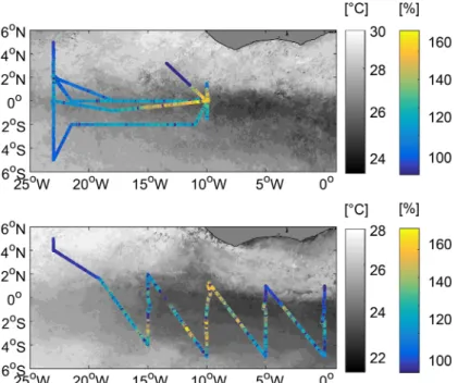
Figure 2.N2O saturation in the EEA in May–July 2011. Distribution map of N2O saturation (right color bars) overlain on monthly mean MODIS-Aqua 4 km SST (left color bars) for May–

June (upper panel, MSM 18-2 cruise) and June–July (lower panel, MSM 18-3 cruise) 2011. Note the different SST scales in Figures 2a and 2b.

(6)

N₂O concentrations (N₂O_calc5 96.9521.22(SST)21.64(SSS)1 0.073(W_sp)) agree well with the concentrations observed during the MSM 18-2 and 18-3 cruises (mean difference<1%; supporting information Figure S1). Fur- thermore, calculated meridional means of N2O concentrations obtained using the same method (linear fit5 217.0220.68(SST)2 1.21(SSS)1 0.069 (W_sp),Ftest,p- value<0.05) also represented well our observations, clearly depicting a sharp eastward increase in surface N2O concentrations with a maximum at about 108W (supporting information Figure S1). The resulting distribution of zonal means for the parameters used in our analysis is shown in Figure 4. Based on the obtained LM equation, dissolved N₂O variability could be explained mostly by SST (up to 97%), whereas the contributions from SSS andW_spwere marginal (former) or non-significant (later;p-value>0.05). Nevertheless, a comparison of N2O and SSS distributions showed that waters in near-equilibrium to undersaturated conditions were almost invariably associated with low SSS and W_sp(Figure 4), in particular when the frontal zone between the NECC and the nSEC at about 28N–38N was crossed. Although the NECC is known to transport low N2O saturation waters from the western basin in association with the Amazon River plume [Lefe`vre et al., 1998;Oudot et al., 2002;Walter et al., 2004], the maximal extent of this plume reaches only 258W–308W [Lefe`vre et al., 2010]. Thus, the source of the low-SSS waters could rather be assigned to high precipitation in the ITCZ during its transit to the north at this time of the year [Philander and Pacanowski, 1986;Xie and Carton, 2004], and dilution caused by such precipitation could then explain the slightly undersaturated waters (down to 96% saturation) which were observed north of the Equator (Figure 4). The lowerW_spobserved north of 38N in the proximity of the ITCZ were consistent with pre- viously reported cross-equatorial wind speed gradients in the tropical Atlantic [Xie, 2005]. However, even thoughW_spis a key factor influencing air-sea gas exchange, its low predictive value for estimating dissolved N2O concentrations in the ACT can be explained by the fact that in this region diapycnal mixing is the main process leading to upward (downward) flux of tracers (heat) [Hummels et al., 2013;Schlundt et al., 2014]. A thorough discussion of the N₂O fluxes at the base of the mixed layer is, however, out of the scope of this manuscript.

Based on our results, the surface distribution of N2O in the EEA could be assigned to two main regimes deﬁned by the location of frontal zones north and south of the Equator. The ‘‘high N₂O’’ regime was characterized by enhanced N2O saturations and cold, salty waters brought to the surface by equatorial upwelling and subsequently advected westward by the nSEC/eSEC. This zonal band with increased N2O (saturation values>100%) was ﬂanked by bands of a ‘‘low N₂O’’ regime with warmer (north and south), fresher (north) waters in which the N2O saturations were close to or slightly below equilibrium (saturation values100%).

From the SST and SSS distributions, it can be inferred that the northern band of the latter regime corre- sponded to the NECC, whereas the southern band coincided with the location of the cSEC.

As mentioned above, averaging the N2O data on a regular grid might have masked small-scale features which could potentially affect its surface distribution. For example, tropical instability waves (TIWs), which are caused by barotropic and baroclinic instability of the equatorial current system [von Schuckmann et al., 2008], resulting in undulations of temperature and salinity fronts, are associated with a distinct pattern of

SST [°C]

22 24 26 28 30

N2O [nmol L-1]

5 6 7 8 9 10 11 12

33.5 34.0 34.5 35.0 35.5 36.0 36.5 SSS

Figure 3.N2O, SST, and SSS in the EEA in May–July 2011. A correlation plot of dissolved N2O and SST for the EEA (58N–58S and 08W–238W) is shown (r²50.87, n549,600). Gray dots represent the equilibrium concentration of N2O computed from in situ SST, SSS, and measured mixing ratios of atmospheric N2O (see section 2.2). The color bar indicates in situ SSS.

(7)

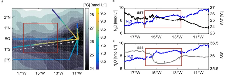
vertical advection and mixing [Menkes et al., 2002; Jochum and Murtugudde, 2006] in the tropical Atlantic and Pacif- ic Oceans [Duing et al., 1975;Flament et al., 1996]. TIWs are known to be a recurrent feature during the seasonal cycle in the tropical Atlantic, being formed in the boreal summer in the central and eastern basin between 58N and 58S, and propagating westward at 0–40 cm s²¹ [Foltz et al., 2004; Athie and Marin, 2008]. Detailed examination of our measurements during the cross- equatorial section EQ II in 10–11 June (Figure 5) revealed that intrusions of warmer, low-SSS waters from the north between about 168W and 138W could be found, and that they partially con- tributed to the observed small-scale ﬂuctuations of N₂O concentrations at the surface. Thus, despite of the clear gradient, with higher N2O concentrations in the eastern side of the EQ II section, intrusion of NECC waters led to marked variations of N₂O during the central part of the transect, after which concentrations started to steadily increase again when approaching the center of the ACT.

The TIWs dominate intraseasonal variability of the surface layer in the tropical Atlantic [Duing et al., 1975].

Moreover they contribute to the biogeochemical tracer and ecosystem variability by altering the SST, nutrient and Chla distributions in such a way that cold, nutrient-rich waters are advected north, thereby enhancing off-equatorial primary production [Menkes et al., 2002].

Due to the close coupling between organic matter production at the surface, sinking and remineralization at depth, and subsurface N2O production [Elkins et al., 1978], it is likely that TIWs also affect the distribution pattern of N2O in the EEA not only by transporting upwelled, N2O-rich waters out of the equatorial upwelling band, but also by enhancing subsurface production north of the Equator. Given the known relevance of TIWs, future studies in this region should assess the overall effect of TIWs on N2O distribution for larger spatial (basin) and temporal (annual cycle) scales as well as the extent at which TIWs might directly impact subsurface N₂O production.

3.3. N2O and Seasonal Development of the ACT

In this section, the 2 month record of continuous N₂O measurements collected during the MSM 18-2 and 18-3 cruises is used to discuss the different phases of the seasonal development of the ACT. According to

5°S 4°S 3°S 2°S 1°S EQ 1°N 2°N 3°N 4°N 5°N 6

8 10

[nmol L-1]

5°S 4°S 3°S 2°S 1°S EQ 1°N 2°N 3°N 4°N 5°N 100

125 150

[%]

5°S 4°S 3°S 2°S 1°S EQ 1°N 2°N 3°N 4°N 5°N 20

25 30

[°C]

5°S 4°S 3°S 2°S 1°S EQ 1°N 2°N 3°N 4°N 5°N 34

35 36

5°S 4°S 3°S 2°S 1°S EQ 1°N 2°N 3°N 4°N 5°N0 5

10

[m s-1]

Wind speed N₂O Saturation

SSS SST N₂O_sw N₂O_air

a

b

c

d

e

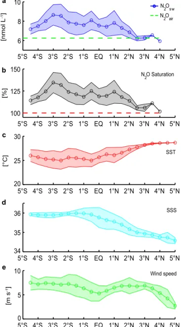
Figure 4.Latitudinal distribution of N2O (a-b), SST (c), SSS (d), and wind speed (e) in the EEA. The line-connected circles represent the mean values per latitudinal band (0.58) for each parameter between 08W and 238W, whereas the shaded areas indicate the corresponding standard deviation. The green dashed line in Figure 4a is the calculated mean equilibrium concentration of N2O in May–July 2011 (6.3 nmol L²¹), and the red dashed line in Figure 4b indicates 100% saturation conditions (i.e., atmospheric equilibrium).

(8)

Caniaux et al. [2011], the onset of the ACT is deﬁned as the date when the surface area in which the SST is lower than 258C exceeds the empirically determined threshold of 0.4 3 10⁶km² (for a spatial domain between 308W–128E and 58N–58S). Based on the work byHormann et al. [2013] who used high-resolution satellite-derived SST data to determine the spatial variability of the ACT, in this study we assume the 29 May as the ACT onset in 2011, which is about 2 weeks earlier than the mean onset date found byCaniaux et al.

[2011].

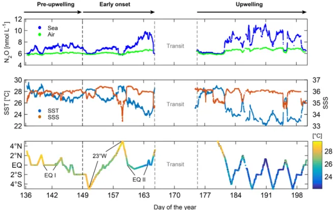
The temporal and spatial variability of dissolved N2O, SST, and SSS in May–July 2011 is shown in Figure 6.

As can be seen, surface N2O follows closely the SST and SSS changes over time, with enhanced concentrations at low SST and close to equilibrium values whenever warm, low-SSS waters from the NECC were present. During the ‘‘pre-upwelling’’ phase (before 29 May) N2O concentrations in the EEA remained close to atmospheric equilibrium (mean6SD 6.960.5 nmol L²¹), ranging between 5.9 and 7.9 nmol L²¹. This pattern was consistent with SST ranging between 26.08C and 29.68C (mean6SD 27.460.78C) and comparatively low wind speeds (not shown). Despite the onset of the ACT on 29 May, low N2O concentrations were observed until the 8 June because during this period the ship occupied the 238W section (between 58N and 58S), where SST were still above 278C (Figure 6).

Hence, the effect of the ACT on surface N₂O was only visible after the 8 June, when a west to east section along the equator was sampled (EQ II, cf. Figure 2). During this ‘‘early onset’’ of the ACT, SST sharply decreased as the ship moved eastward reaching a minimum of 23.58C at about 108W. This temperature gradient was in phase with changes in N2O, such that concentrations increased by 22% with respect to those of the ‘‘pre-upwelling phase’’ (early onset mean: 8.0 nmol L²¹; cf. Figure 6). For comparison, N2O concentrations during the EQ I section (which took place before the ACT onset) were 16% lower than in EQ II. Thus, although SST and N2O gradients were observed both in EQ I and EQ II, the latter provided indication of an upwelling-driven increase in surface N₂O concentrations.

After a transit period of about 10 days, the continuous measurements were resumed and a series of cross- equatorial sections between 208W and 08E was carried out from 1 to 19 July. At this stage a well-developed ACT could be observed, with low SST (minimum 22.18C) centered between 28S and the Equator, and at 108W [see alsoSchlundt et al., 2014]. These conditions indicated the occurrence of equatorial upwelling, which, as can be seen in Figure 6, was associated with an important enhancement in surface N₂O concentrations in the ACT region with respect to the pre-upwelling phase in early May.

Thus, N₂O concentrations were generally low (at or near atmospheric equilibrium) during the warm period preceding the onset of the ACT (early May), in particular toward 238W where the SST were the highest.

Then, cooling associated with the onset of the ACT during late May/early June led to a moderate increase in N2O concentrations at the Equator with the highest values toward the center of the ACT at 108W. Finally,

17°W 15°W 13°W 11°W

6 8 10

N2O [nmol L-1]

23 24 25 26 27

SST [°C]

17°W 15°W 13°W 11°W

6 8 10

35.5 36 36.5

SSS

17°W 15°W 13°W 11°W 2°S

1°S EQ 1°N 2°N

24 25 26 27 28

6.5 7.0 7.5 8.0 8.5 9.0 9.5 [°C] [nmol L^-1]

N₂O SST

N₂O SSS

a b

N2O [nmol L-1]

c

Figure 5.Small-scale variability of surface N2O in the EEA. (a) Daily mean SST map (resolution 0.25830.258) for 10–11 June 2011 (contours) overlaid by N2O concentrations from the MSM 18-2 cruise (circles). (b, c) N2O, SST, and SSS distribution along the equatorial section EQ II, which was crossed on the same dates as in Figure 5a. EQ II section is indicated by the white dashed arrow in Figure 5a, whereas the TIW feature is highlighted by a red square in Figures 5a–5c.

(9)

during July a fully developed ACT could be observed and it was associated with the highest N2O concentrations during our sampling period. Our observations also show that the N₂O distribution in the EEA reﬂected the spatial pattern of equatorial upwelling, which is particularly strong south of the Equator and in the vicin- ity of 108W [Grodsky et al., 2008;Caniaux et al., 2011].

3.4. N2O at Depth and Source of Upwelling Waters

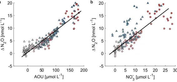
Similar to previous studies in the tropical Atlantic [Oudot et al., 2002;Forster et al., 2009], we found the highest N2O concentrations (up to 30 nmol L²¹) to be associated with the South Atlantic Central Water (SACW) at depths from 150 to 500 m (r526.46–27.02 kg m²³) [Poole and Tomczak, 1999;Stramma and England, 1999]. Likewise, based on data from selected stations (EQ I and EQ II sections), we also observed good corre- lations both betweenDN2O and AOU, and betweenDN2O and NO²₃ concentrations in the water column (Figure 7), which suggests that the N₂O observed at the surface was produced by microbial nitrification at depth [Elkins et al., 1978]. This is in line with the results fromFrame et al. [2014], who observed a N2O concentration maximum at 200–400 m (along 128S) to be associated with combined nitrification and nitrifier denitrification carried out by ammonia oxidizers. However, the extent at which the latter process could have had an influence in our results cannot be assessed from our data.

OurDN₂O/AOU slope of 0.08 agrees well with the values reported byWalter et al. [2006] for waters<500 m depth, whereas theDN2O/NO²₃ slope is somewhat lower than in their study, probably indicating mixing of waters with different N₂O concentrations. Our observedDN₂O/AOU slope is, however, lower than those reported byOudot et al. [2002] andForster et al. [2009].Oudot et al. [2002] suggested enhanced primary production from coastal upwelling on the eastern basin of the tropical Atlantic as the reason for their comparatively high DN₂O/AOU correlation slopes. However, Walter et al. [2006] argued that the increased productivity on the EEA for that period (October) is rather due to dust deposition and riverine inputs.

Although we only considered the near-equatorial data (i.e., 08S–28S) in this analysis, it could be hypothe- sized that during the equatorial upwelling a high amount of sinking organic matter could stimulate

Figure 6.Onset and development of the ACT in 2011. Seawater (dark blue) and atmospheric (green) concentrations of N2O (upper panel), as well as in situ SST and SSS (light blue and red, respectively; middle panel) during different phases of the seasonal progression of the ACT are shown. Ship’s position and in situ SST during the MSM 18-2 and 18-3 cruises are also shown (lower panel). The black dashed lines depict the estimated onset of the ACT [Hormann et al., 2013], whereas the gray dashed lines indicate a transit period between the two cruises. The position and timing of selected along and cross-equatorial sections (EQ I, EQ II and 238W, cf. Figure 1) are indicated in the lower panel. Days of the year (DOY) 136 and 198516 May and 17 July, respectively.

(10)

enhanced respiration in the water column, thereby reducing O2concentrations and leading to enhanced N2O yields from nitriﬁcation [Elkins et al., 1978]. Further analysis of the DN2O/AOU relationship for the EEA based on expedition data is therefore required in order to assess the impact of equatorial upwelling in the subsurface variability of N₂O. In particular, meridional gradients in the distribution of phytoplankton communities should be considered since the highest abundances tend to be concentrated at 0.58–18 north/south of the Equator [Vinogradov, 1981]. Hence, an upwelling-driven increase of organic material that could potentially sink and fuel subsurface N-cycling might take place a few degrees off rather than directly at the Equator. Likewise, the role of the locally produced nitriﬁcation-derived N₂O versus N₂O that is advected from deep waters over longer time scales than in our survey should also be addressed in future studies.

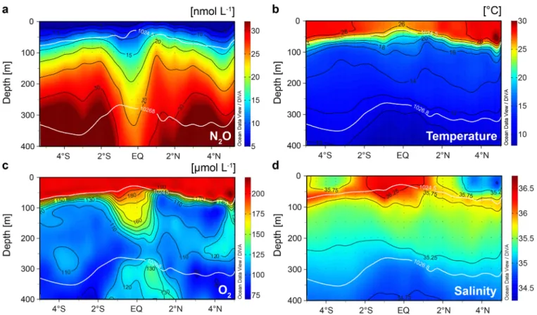
Figure 8 shows the cross-equatorial vertical distribution of N₂O, O₂as well as temperature and salinity for a south–north section along 238W (cf. Figure 1). As can be seen, the meridional gradients of SST and SSS observed at the surface (i.e., high SST, low SSS north of 2–38N) could be also detected for the upper meters of the water column. In general, N2O featured a pronounced maximum at about 300–400 m, consistent with an O₂minimum of about 80lmol L²¹in the same depth range. This is in agreement with the vertical distribution reported by previous studies in the tropical Atlantic [Oudot et al., 2002; Walter et al., 2006;

Forster et al., 2009]. However, two subsurface O2maxima with concentrations>130lmol L²¹could be iden- tiﬁed close to the Equator; the ﬁrst was located near the surface at depths down to150 m whereas the second could be observed at 300–400 m. N₂O concentrations were lower within these high-O₂‘‘plumes’’

than in surrounding waters, further supporting the goodDN₂O/AOU correlation found along the equatorial sections EQ I and EQ II, and the nitrification source of N2O in the central and east region of the equatorial Atlantic. The upper subsurface high-O2plume was centered at about 28S–28N, and within the isopycnal surfaces which define the EUC [Hormann and Brandt, 2007]. The EUC flows eastward with the highest velocities in boreal spring and autumn [Brandt et al., 2014], carrying cold and saline waters with elevated O₂concentrations to the EEA [Hormann and Brandt, 2007;Brandt et al., 2014;Schlundt et al., 2014]. Vertical distribution of temperature and salinity also support this argument, with uplifting of isotherms and a salinity maximum directly at the Equator (Figure 8). The second O2maximum was located below the EUC and can be attributed to an eastward-flowing equatorial jet. Such jets are a known pathway for the transport of high-O₂waters to the EEA [Brandt et al., 2008, 2012], and as it is shown in Figure 8 they could be associated with comparatively lower N2O concentrations at depth in the equatorial band. Unlike O2however, the N2O distribution does not feature a clearly defined separation between upper (150 m) and lower (350 m) minima, but a rather uniform band with comparatively low N₂O concentrations (25 nmol L²¹). This pattern could also be observed at 108W, where the deep (350 m) O₂maximum is displaced further south from the N₂O minimum (see supporting information Figure S2), suggesting that the zonal advection along the equator might have

0 5 10 15 20 25 30

NO₃^- [μmol L^-1] -5

0 5 10 15 20

∆N 2O [nmol L-1 ]

0 50 100 150 200

AOU [μmol L^-1] -5

0 5 10 15 20

∆N 2O [nmol L-1 ]

a b

Figure 7.DN2O/AOU andDN2O/NO²₃relationships for selected stations in the EEA. Correlation plots of (a)DN2O versus AOU and (b)DN2O versus NO²₃ from equatorial sections EQ I (circles) and EQ II (triangles) are shown. The regression lines for Figures 7a (DN2O50.083(AOU)10.879, r²50.86, n5230) and 7b (DN2O50.564(NO²₃)12.735, r²50.56, n5298) are depicted in black, and the symbol color intensity represents in situ O2concentrations (lighter colors indicate higher values).

(11)

a stronger effect for O₂than for N₂O, most likely indicating slower subsurface N₂O production in comparison with the O2supply rates directly at the Equator.

In summary, our observations suggest that in the EEA N₂O is produced in thermocline waters by nitriﬁcation and is then partially advected and mixed to the surface during equatorial upwelling. This source of N2O to the surface is, however, not homogeneous because the upwelling is stronger to the south of the Equator [Caniaux et al., 2011]. Likewise, we observed that surface N₂O concentrations directly at the equator are lower than in off-equatorial locations within the ACT region since the relatively N₂O-poor, O₂-rich EUC is the main source of upwelled waters in the EEA.

3.5. Sea-to-Air Fluxes of N₂O

N2O flux densities (F_N₂_O) in the EEA were mostly positive at the time of sampling, indicating net outgassing of N2O to the atmosphere during the onset and development of the ACT.F_N₂_Ovalues were, however, highly variable ranging between20.60 and 20.74lmol m²²d²¹(mean6SD 3.4662.59lmol m²²d²¹). These fluctuations reflect the spatial and temporal variability in SST and wind speeds, and their interplay with N₂O concentrations at the surface. Thus, the highest N2O flux densities were found in the zonal band between 28N and 48S, extending from the center of the ACT at 108W [Grodsky et al., 2008;Schlundt et al., 2014] to about 158W. Although relatively weak, the zonal (meridional) gradients ofF_N₂_Owere consistent with SST gradients of 0.28C per degree longitude (latitude) (i.e., highF_N₂_Owhere the lowest SST were found). Contrarily, east of 108W and north of 28N, we found comparatively lower F_N₂_O. North of the Equator this can be explained by warm (>268C), near-equilibrium to undersaturated waters in conjunction with reduced wind speeds, whereas east of 108W this result might be rather due to low wind speeds and not to SST, because the sampling in this area took place after the onset of the ACT (16–17 July). Likewise,Hummels et al. [2014]

observed reduced diapycnal mixing east of 108W in the ACT region, which suggests a decreased transport of N₂O toward the surface. Our computedF_N₂_Ovalues are (in the mean) higher than those from previous studies (0.61–2.13lmol m²²d²¹) [see e.g.,Oudot et al., 2002;Walter et al., 2004;Forster et al., 2009]. These

Figure 8.Depth distribution of N2O, O2, temperature, and salinity at 238W. A cross-equatorial section of (a) N2O and (c) O2concentrations as well as (b) temperature and (d) salinity along 238W is shown. The potential density (r) surfaces 24.5 and 26.8 kg m²³are indicated as white contours.

(12)

differences can be explained both by the use of different gas exchange parameterizations and by the fact that the magnitude of the sea-to-air concentration differences measured in this study were markedly higher. Hence, the onset of the ACT and the associated changes in SST and enhanced wind speeds along and across the Equator led to increased sea-to-air ﬂuxes of N2O.

In order to differentiate between N₂O ﬂuxes from the ACT and from adjacent locations within the EEA, we used the SST criterion ofCaniaux et al. [2011], whereby ACT and off-ACT regions are separated based on a 258C threshold (ACT5waters where SST<258C). It is worth noting that N₂O ﬂuxes from the ACT doubled those from the area out of the ACT (mean6SD 5.1862.59 and 2.5961.73lmol m²²d²¹, respectively), thus highlighting the role of the equatorial upwelling in enhancing outgassing of N₂O in the EEA. From this, it follows that the EEA is a moderate source of this GHG to the atmosphere, which is comparable with, for instance, the coastal upwelling system off Mauritania [seeKock et al., 2012]. Nevertheless, it should be pointed out that the ACT is characterized by strong seasonal and interannual variability [Caniaux et al., 2011;

Hormann et al., 2013], and therefore its share to the annual ﬂuxes of N2O is also object of some variability.

Sustained observations in platforms such as moorings and vessels of opportunity [see e.g.,Lefe`vre et al., 2008, 2014] could thus help to disentangle the long-term trends in the N2O distribution and to assess the extent of the annual variability of the emissions.

4. Summary and Conclusion

Our results represent the first detailed investigation of the distribution and sea-to-air fluxes of N₂O during the onset and development of the ACT. We found that surface concentrations of N2O are closely linked to SST and, at a minor extent, to SSS and wind speeds, resulting in ‘‘high’’ and ‘‘low’’ concentration regimes which are delimited by the spatial extent of the NECC and SEC, as well as the occurrence of equatorial upwelling. Based on our observations, we suggest that N₂O reaching the surface ocean at the time of sampling was derived from subsurface production through nitrification and vertical fluxes (advection and mixing) during the upwelling season. Moreover, the onset and seasonal development of the ACT could be clearly observed in the surface distribution of N₂O, with concentrations increasing progressively as the seasonal cooling in the equatorial region proceeded during spring–summer 2011. In addition to the regional variability, TIWs modulate the surface distribution of N₂O by meridionally advecting N₂O-rich (poor) waters out of (into) the equatorial divergence. The EEA was a moderate source of N2O to the atmosphere at the time of sampling despite the seasonal enhancement of concentrations and sea-to-air fluxes associated with the ACT. However, interannual variability of the onset, duration and extent of the ACT could also influence the fluctuations in N₂O fluxes out of the EEA.

In conclusion, this study evidenced that the onset of the ACT leads to an enhancement of surface N2O concentrations in the EEA, mostly due to the transport of cold, N₂O-rich waters from the thermocline into the surface. Nevertheless, our measurements only cover part of the seasonal cycle in the EEA and therefore many open questions remain as to which are the effects of the intraseasonal and interannual variability of the ACT in the N2O distribution and emissions to the atmosphere.

References

Arevalo-Martınez, D. L., M. Beyer, M. Krumbholz, I. Piller, A. Kock, T. Steinhoff, A. K€ortzinger, and H. W. Bange (2013), A new method for continuous measurements of oceanic and atmospheric N2O, CO and CO2: Performance of off-axis-integrated cavity output spectroscopy (OA-ICOS) coupled to non-dispersive infrared detection (NDIR),Ocean Sci.,9, 1071–1087.

Athie, G., and F. Marin (2008), Cross-equatorial structure and temporal modulation of intraseasonal variability at the surface of the Tropical Atlantic Ocean,J. Geophys. Res.,113, C08020, doi:10.1029/2007JC004332.

Bindoff, N. L., et al. (2013), Detection and attribution of climate change: From global to regional, inClimate Change 2013: The Physical Sci- ence Basis, Contribution of Working Group I to the Fifth Assessment Report of the Intergovernmental Panel on Climate Change, edited by T. F. Stocker et al., pp. 867–952, Cambridge Univ. Press, Cambridge, U. K.

Brandt, P., V. Hormann, B. Bourle`s, J. Fischer, F. A. Schott, L. Stramma, and M. Dengler (2008), Oxygen tongues and zonal currents in the equatorial Atlantic,J. Geophys. Res.,113, C04012, doi:10.1029/2007JC004435.

Brandt, P., G. Caniaux, B. Bourle`s, A. Lazar, M. Dengler, A. Funk, V. Hormann, H. Giordani, and F. Marin (2011), Equatorial upper-ocean dynamics and their interaction with the West African monsoon,Atmos. Sci. Let.,12, 24–30.

Brandt, P., R. J. Greatbatch, M. Claus, S.-H. Didwischus, V. Hormann, A. Funk, G. Krahmann, J. Fischer, and A. Kortzinger (2012), Ventilation of the equatorial Atlantic by the equatorial deep jets,J. Geophys. Res.,117, C12015, doi:10.1029/2012JC008118.

Brandt, P., A. Funk, A. Tantet, W. E. Johns, and J. Fischer (2014), The equatorial undercurrent in the central Atlantic and its relation to tropical Atlantic variability,Clim. Dyn.,43, 2985, doi:10.1007/s00382-014-2061-4.

Acknowledgments

This study was funded by the BMBF joint projects NORDATLANTIK and SOPRAN II (FKZ 03F0611A), the DFG- supported Collaborative Research Center SFB754 (http:www.sfb754.de), the Future Ocean Excellence Cluster at Kiel University (project CP0910), and the EU FP7 project InGOS (grant agreement 284274). We are very grateful to the captain and crew of the R/V Maria S. Merian for their assistance during the MSM 18-2 and 18-3 cruises.

Likewise, we thank A. Jordan for the calibration of our standard gases at the Max Planck Institute for Biogeochemistry in Jena. We also thank B. Fiedler, T. Baustian, and M. Krumbholz for providing technical support to the continuous measurements of N2O and the sampling/measurement of discrete N2O samples during MSM 18-3.

Moreover, we thank M. Lohmann and N. Martogli for providing O2and nutrient data, as well as G. Krahmann and M. Schlundt for their contribution to the processing of CTD and thermosalinograph data. Figure 1 was produced by using monthly means of MODIS-Aqua SST at a resolution of 4 km. This data set was retrieved from the Goddard Earth Sciences Data and Information Services Center (GES DISC, http://disc.sci.gsfc.nasa.gov/giovanni/).

Discrete and underway N2O data collected during the MSM 18-2 and 18- 3 cruises will be archived in the MEMENTO (MarinE MethanE and NiTrous Oxide) database (http://portal.

geomar.de/web/memento/home) upon publication.

(13)

Caniaux, G., H. Giordani, J.-L. Redelsperger, F. Guichard, E. Key, and M. Wade (2011), Coupling between the Atlantic cold tongue and the West African monsoon in boreal spring and summer,J. Geophys. Res.,116, C04003, doi:10.1029/2010JC006570.

Carton, J. A., X. Cao, B. J. Giese, and A. M. Da Silva (1996), Decadal and interannual SST variability in the tropical Atlantic Ocean,J. Phys. Oce- anogr.,26, 1165–1175.

Chang, P., et al. (2006), Climate ﬂuctuations of tropical coupled systems—The role of ocean dynamics,J. Clim.,19(20), 5122–5174, doi:

10.1175/JCLI3903.1.

Christian, J. R., and R. Murtugudde (2003), Tropical Atlantic variability in a coupled physical-biogeochemical ocean model,Deep Sea Res., Part II,50, 2947–2969.

Ciais, P., et al. (2013), Carbon and other biogeochemical cycles, inClimate Change 2013: The Physical Science Basis, Contribution of Working Group I to the Fifth Assessment Report of the Intergovernmental Panel on Climate Change, pp. 465–570, Cambridge Univ. Press, Cambridge, U. K.

Duing, W., P. Hisard, E. Katz, J. Meincke, L. Miller, K. V. Moroshkin, G. Philander, A. A. Ribnikov, K. Voigt, and R. Weisberg (1975), Meanders and long waves in the equatorial Atlantic,Nature,257, 280–284.

Dlugokencky, E. J., P. M. Lang, and K. A. Masarie (2011),Atmospheric N2O dry air mole fractions from the NOAA GMD Carbon Cycle Coopera- tive Global Air Sampling Network, 1997–2010, Version: 2011-11-09, U.S. Department of Commerce, National Oceanic and Atmospheric Administration (NOAA).

Elkins, J. W., S. C. Wofsy, M. B. McElroy, C. E. Kolb, and W. A. Kaplan (1978), Aquatic sources and sinks for nitrous oxide,Nature,275, 602–606.

Flament, P. J., S. C. Kennan, R. A. Knox, P. A. Niiler, and R. L. Bernstein (1996), The three-dimensional structure of an upper ocean vortex in the equatorial Paciﬁc Ocean,Nature,383, 610–613.

Foltz, G. R., J. A. Carton, and E. P. Chassignet (2004), Tropical instability vortices in the Atlantic Ocean,J. Geophys. Res.,109, C03029, doi:

10.1029/2003JC001942.

Forster, G., R. C. Upstill-Goddard, N. Gist, C. Robinson, G. Uher, and E. M. S. Woodward (2009), Nitrous oxide and methane in the Atlantic Ocean between 508N and 528S: Latitudinal distribution and sea-to-air ﬂux,Deep Sea Res., Part II,56, 964–976.

Frame, C. H., E. Deal, C. D. Nevison, and K. L. Casciotti (2014), N2O production in the eastern South Atlantic: Analysis of N2O stable isotopic and concentration data,Global Biogeochem. Cycles,28, 1262–1278, doi:10.1002/2013GB004790.

Garbe, C. S., et al. (2014), Transfer across the air-sea interface, inOcean-Atmosphere Interactions of Gases and Particles, edited by P. S. Liss, and M. T. Johnson, pp. 55–112, Springer, Berlin.

Garrat, J. R. (1977), Review of drag coefﬁcients over oceans and continents,Mon. Weather Rev.,105, 915–929.

Grefe, I., and J. Kaiser (2014), Equilibrator-based measurements of dissolved nitrous oxide in the surface ocean using an integrated cavity output laser absorption spectrometer,Ocean Sci.,10, 501–512, doi:10.5194/os-10-501-2014.

Grodsky, S. A., J. A. Carton, and C. R. McClain (2008), Variability of upwelling and chlorophyll in the equatorial Atlantic,Geophys. Res. Lett., 35, L03610, doi:10.1029/2007GL032466.

Hansen, H. P. (1999), Determination of oxygen, inMethods of Seawater Analysis, edited by K. G. Grasshoff, K. Kremling, and M. Ehrhardt, pp. 75–90, Wiley-VCH, Weinheim, Germany.

Hartmann, D. L., et al. (2013), Observations: Atmosphere and surface, inClimate Change 2013: The Physical Science Basis, Contribution of Working Group I to the Fifth Assessment Report of the Intergovernmental Panel on Climate Change, edited by T. F. Stocker et al., pp. 159–

254, Cambridge Univ. Press, Cambridge, U. K.

Hormann, V., and P. Brandt (2007), Atlantic Equatorial Undercurrent and associated cold tongue variability,J. Geophys. Res.,112, C06017, doi:10.1029/2006JC003931.

Hormann, V., R. Lumpkin, and R. C. Perez (2013), A generalized method for estimating the structure of the Equatorial Atlantic cold tongue:

Application to drifter observations,J. Atmos. Oceanic. Technol.,30, 1884–1895, doi:10.1175/JTECH-D-12-00173.1.

Hummels, R., M. Dengler, and B. Bourle`s (2013), Seasonal and regional variability of upper ocean diapycnal heat ﬂux in the Atlantic cold tongue,Prog. Oceanogr.,111, 52–74, doi:10.1016/j.pocean.2012.11.001.

Hummels, R., M. Dengler, P. Brandt, and M. Schlundt (2014), Diapycnal heat ﬂux and mixed layer heat budget within the Atlantic Cold Tongue,Clim. Dyn.,43, 3179–3199, doi:10.1007/s00382-014-2339-6.

Hydes, D. J., et al. (2010), Recommendations for the determination of nutrients in seawater to high levels of precision and inter-comparability using continuous ﬂow analysers, inThe GO-SHIP Repeat Hydrography Manual: A Collection of Expert Reports and Guidelines, edited by E. M. Hood, C. L. Sabine, and B. M. Sloyan,IOCCP Rep. 14, ICPO Publ. Ser. 134, International Ocean Carbon Coordination Project (IOCCP).

[Available at http://www.go-ship.org/HydroMan.html.]

Jochum, M., and R. Murtugudde (2006), Temperature advection by tropical instability waves,J. Phys. Oceanogr.,36, 592–605.

Kock, A., J. Schafstall, M. Dengler, P. Brandt, and H. W. Bange (2012), Sea-to-air and diapycnal nitrous oxide ﬂuxes in the eastern tropical North Atlantic Ocean,Biogeosciences,9, 957–964.

Lefe`vre, N., G. Moore, J. Aiken, A. Watson, D. Cooper, and R. Ling (1998), Variability ofpCO2in the tropical Atlantic in 1995,J. Geophys. Res., 103(C3), 5623–5634.

Lefe`vre, N., A. Guillot, L. Beaumont, and T. Danguy (2008), Variability offCO2in the Eastern Tropical Atlantic from a moored buoy,J. Geo- phys. Res.,113, C01015, doi:10.1029/2007JC004146.

Lefe`vre, N., D. Diverre`s, and F. Gallois (2010), Origin of CO2undersaturation in the western tropical Atlantic,Tellus, Ser. B,62B(5), 595–607.

Lefe`vre, N., D. F. Urbano, F. Gallois, and D. Diverre`s (2014), Impact of physical processes on the seasonal distribution of the fugacity of CO2

in the western tropical Atlantic,J. Geophys. Res. Oceans,119, 646–663, doi:10.1002/2013JC009248.

Lumpkin, R., and S. L. Garzoli (2005), Near-surface circulation in the Tropical Atlantic Ocean,Deep Sea Res., Part I,52, 495–518.

Menkes, C. E., et al. (2002), A whirling ecosystem in the equatorial Atlantic,Geophys. Res. Lett.,29(11), 1553, doi:10.1029/2001GL014576.

Nevison, C. D., R. F. Weiss, and D. J. Erikson III (1995), Global oceanic emissions of nitrous oxide,J. Geophys. Res.,100(C8), 15,809–15,820.

Nightingale, P. D., G. Malin, C. S. Law, A. J. Watson, P. S. Liss, M. I. Liddicoat, J. Boutin, and R. C. Upstill-Goddard (2000), In situ evaluation of air-sea gas exchange parameterizations using novel conservative and volatile tracers,Global Biogeochem. Cycles,14(1), 373–387.

Oudot, C., C. Andrie, and Y. Montel (1990), Nitrous oxide production in the tropical Atlantic Ocean,Deep Sea Res., Part A,37(2), 183–202.

Oudot, C., P. Jean-Baptiste, E. Fourre, C. Mormiche, M. Guevel, J.-F. Ternon, and P. Le Corre (2002), Transatlantic equatorial distribution of nitrous oxide and methane,Deep Sea Res., Part I.,49, 1175–1193.

Philander, S. G. H., and R. C. Pacanowski (1986), A model of the seasonal cycle in the tropical Atlantic Ocean,J. Geophys. Res.,91(C12), 14,192–14,206.

Poole, R., and M. Tomczak (1999), Optimum analysis of the water mass structure in the Atlantic Ocean thermocline,Deep Sea Res., Part I., 46, 1895–1921.

Ravishankara, A. R., J. S. Daniel, and R. W. Portmann (2009), Nitrous oxide (N2O): The dominant ozone-depleting substance emitted in the 21st Century,Science,326, 123–125.

(14)

Rhee, T. S., A. J. Kettle, and M. O. Andreae (2009), Methane and nitrous oxide emissions from the ocean: A reassessment using basin-wide observations in the Atlantic,J. Geophys. Res.,114, D12304, doi:10.1029/2008JD011662.

Schlundt, M., P. Brandt, M. Dengler, R. Hummels, T. Fischer, K. Bumke, G. Krahmann, and J. Karstensen (2014), Mixed layer heat and salinity budgets during the onset of the 2011 Atlantic cold tongue,J. Geophys. Res. Oceans,119, 7882–7910, doi:10.1002/2014JC010021.

Stramma, L., and M. England (1999), On the water masses and mean circulation of the South Atlantic Ocean,J. Geophys. Res.,104(C9), 20,863–20,883.

Stramma, L., and F. Schott (1999), The mean ﬂow ﬁeld of the tropical Atlantic Ocean,Deep Sea Res., Part II,46, 279–303.

Takahashi, T., et al. (2009), Climatological mean and decadal change in surface oceanpCO2, and net sea-air CO2ﬂux over the global oceans, Deep Sea Res., Part II,56, 554–577.

Tokinaga, H., and S. Xie (2011), Weakening of the equatorial Atlantic cold tongue over the past six decades,Nat. Geosci.,4, 222–225.

Vinogradov, M. (1981), Ecosystems of equatorial upwellings, inAnalysis of Marine Ecosystems, edited by A. R. Longhurst, pp. 69–93, Aca- demic, London, U. K.

Voituriez, B. (1981), Equatorial upwelling in the Eastern Atlantic: Problems and paradoxes, inCoastal Upwelling, edited by F. A. Richards, pp. 95–106, AGU, Washington, D. C.

Von Schuckmann, K., P. Brandt, and C. Eden (2008), Generation of tropical instability waves in the Atlantic Ocean,J. Geophys. Res.,113, C08034, doi:10.1029/2007JC004712.

Walter, S., H. W. Bange, and D. W. R. Wallace (2004), Nitrous oxide in the surface layer of the tropical North Atlantic Ocean along a west to east transect,Geophys. Res. Lett.,31, L23S07, doi:10.1029/2004GL019937.

Walter, S., H. W. Bange, U. Breitenbach, and D. W. R. Wallace (2006), Nitrous oxide in the North Atlantic Ocean,Biogeosciences,3, 607–619.

Weiss, R. F., and B. A. Price (1980), Nitrous oxide solubility in water and seawater,Mar. Chem.,8, 347–359.

Weiss, R. F., F. A. Van Woy, and P. K. Salameh (1992), Surface water and atmospheric carbon dioxide and nitrous oxide observations by shipboard automated gas chromatography: Results from expeditions between 1977 and 1990,Scripps Inst. Oceanogr. Ref. 92–11, Scripps Inst. of Oceanogr., San Diego, Calif.

Xie, S.-P. (2005), The shape of continents, air-sea interaction, and the rising branch of the Hadley circulation, inThe Hadley Circulation:

Present, Past and Future, edited by H. F. Diaz and R. S. Bradley, pp. 121–152, Kluwer Acad., Dordrecht, Netherlands.

Xie, S.-P., and J. A. Carton (2004), Tropical Atlantic variability: Patterns, mechanisms, and impacts, inEarth Climate: The Ocean-Atmosphere Interaction, Geophys. Monogr., edited by C. Wang, S.-P. Xie, and J. A. Carton, pp. 121–142, AGU, Washington, D. C.