Dissolved organic matter at the fluvial–marine transition in the Laptev Sea using in situ data and ocean colour remote sensing

Biogeosciences, 16, 2693–2713, 2019 https://doi.org/10.5194/bg-16-2693-2019

© Author(s) 2019. This work is distributed under the Creative Commons Attribution 4.0 License.

Dissolved organic matter at the fluvial–marine transition in the Laptev Sea using in situ data and ocean colour remote sensing

Bennet Juhls¹, Pier Paul Overduin², Jens Hölemann³, Martin Hieronymi⁴, Atsushi Matsuoka⁵, Birgit Heim², and Jürgen Fischer¹

1Institute for Space Sciences, Department of Earth Sciences, Freie Universität Berlin, Berlin, Germany

2Alfred Wegener Institute Helmholtz Centre for Polar and Marine Research, Potsdam, Germany

3Alfred Wegener Institute Helmholtz Centre for Polar and Marine Research, Bremerhaven, Germany

4Institute of Coastal Research, Helmholtz-Zentrum Geesthacht, Geesthacht, Germany

5Takuvik Joint International Laboratory, Département de Biologie, Université Laval, Québec City, Canada Correspondence:Bennet Juhls (bjuhls@wew.fu-berlin.de)

Received: 27 February 2019 – Discussion started: 1 March 2019

Revised: 9 June 2019 – Accepted: 17 June 2019 – Published: 11 July 2019

Abstract.River water is the main source of dissolved organic carbon (DOC) in the Arctic Ocean. DOC plays an important role in the Arctic carbon cycle, and its export from land to sea is expected to increase as ongoing climate change ac- celerates permafrost thaw. However, transport pathways and transformation of DOC in the land-to-ocean transition are mostly unknown. We collected DOC andaCDOM(λ)samples from 11 expeditions to river, coastal and offshore waters and present a new DOC–aCDOM(λ)model for the fluvial–marine transition zone in the Laptev Sea. The aCDOM(λ) charac- teristics revealed that the dissolved organic matter (DOM) in samples of this dataset are primarily of terrigenous ori- gin. Observed changes ina_CDOM(443) and its spectral slopes indicate that DOM is modified by microbial and photo- degradation. Ocean colour remote sensing (OCRS) provides the absorption coefficient of coloured dissolved organic mat- ter (a_CDOM(λ)^sat) atλ=440 or 443 nm, which can be used to estimate DOC concentration at high temporal and spatial resolution over large regions. We tested the statistical per- formance of five OCRS algorithms and evaluated the plau- sibility of the spatial distribution of derived aCDOM(λ)^sat. The OLCI (Sentinel-3 Ocean and Land Colour Instrument) neural network swarm (ONNS) algorithm showed the best performance compared to in situ aCDOM(440) (r²=0.72).

Additionally, we found ONNS-derivedaCDOM(440), in con- trast to other algorithms, to be partly independent of sediment concentration, making ONNS the most suitablea_CDOM(λ)^sat algorithm for the Laptev Sea region. The DOC–a_CDOM(λ)

model was applied to ONNS-deriveda_CDOM(440), and re- trieved DOC concentration maps showed moderate agree- ment to in situ data (r²=0.53). The in situ and satellite- retrieved data were offset by up to several days, which may partly explain the weak correlation for this dynamic region.

Satellite-derived surface water DOC concentration maps from Medium Resolution Imaging Spectrometer (MERIS) satellite data demonstrate rapid removal of DOC within short time periods in coastal waters of the Laptev Sea, which is likely caused by physical mixing and different types of degradation processes. Using samples from all occurring wa- ter types leads to a more robust DOC–a_CDOM(λ)model for the retrievals of DOC in Arctic shelf and river waters.

1 Introduction

Large volumes of freshwater (3588±257 km³yr⁻¹; Syed et al., 2007) and dissolved organic matter (DOM) (25–

36 Tg C yr⁻¹) (Raymond et al., 2007) are discharged by Arc- tic rivers into the Arctic Ocean (Cooper et al., 2005; Dittmar and Kattner, 2003; Stedmon et al., 2011). Recent studies predict an increase of DOM flux to the Arctic Ocean with continued climate warming and permafrost thawing (Camill, 2005; Freeman et al., 2001; Frey and Smith, 2005). This will lead to a cascade of effects on the physical, chemical and biological environment of Arctic shelf waters (Stedmon et al., 2011). These include an increase of radiative heat trans-

fer into surface waters, changes in carbon sequestration and reductions of sea-ice extent and thickness (Hill, 2008; Mat- suoka et al., 2011).

The Laptev Sea is a wide shelf sea in the eastern Arctic, characterized by fresh surface waters from the Lena River, which delivers around one-fifth (609.5±59 km³yr⁻¹) of all river water to the Arctic Ocean (Bauch et al., 2013; Fe- dorova et al., 2015; Stedmon et al., 2011). River water is the main source of DOM and thus of dissolved organic carbon (DOC) and coloured dissolved organic matter (CDOM) to the Laptev Sea shelf (Cauwet and Sidorov, 1996; Gonçalves- Araujo et al., 2015; Kattner et al., 1999; Lobbes et al., 2000;

Thibodeau et al., 2014; Vantrepotte et al., 2015). Moreover, the Lena River has the highest peak concentrations of DOC of up to 1600 µmol L⁻¹ (Stedmon et al., 2011) of all Arc- tic rivers. The fate and transformation of DOM as it is dis- charged to the Arctic Ocean, however, are not well known.

Physical and biological processes, such as photodegradation (Gonçalves-Araujo et al., 2015; Helms et al., 2008, 2014;

Opsahl and Benner, 1997) and microbial degradation (Ben- ner and Kaiser, 2011; Fasching et al., 2015; Fichot and Ben- ner, 2014; Matsuoka et al., 2012, 2015), as well as miner- alization (Kaiser et al., 2017) and flocculation (Asmala et al., 2014; Guo et al., 2007), are responsible for the modifica- tion and removal of DOM from river-influenced surface wa- ters. Given the strong seasonality of Lena River runoff (Yang et al., 2002), DOC concentration varies greatly in time and space (Amon et al., 2012; Cauwet and Sidorov, 1996; Ray- mond et al., 2007; Stedmon et al., 2011). Once exported to the sea, rapid transport of water masses and dislocation of fronts cause rapid changes in concentrations of surface water constituents at any given location.

Therefore, DOC sampling at high temporal and spatial res- olutions over long periods is necessary to understand these changes. Discrete in situ sampling of DOC during expedi- tions provides point measurements at the time of sampling and is complicated by the difficulty of accessing shallow water for ocean-going vessels. The resulting inadequacy of sample coverage in space and time can be overcome by us- ing ocean colour remote sensing (OCRS) data. The absorp- tion coefficient of CDOM (a_CDOM(λ)) at a reference wave- length λ (usuallyλ=443 nm orλ=440 nm is used) is an optical property of the water and can also be derived with OCRS during ice and cloud-free periods. Hereinafter, we re- fer to satellite-derivedaCDOM(λ) asaCDOM(λ)^sat. CDOM ab- sorbs light in the ultraviolet and visible wavelengths (Green and Blough, 1994) and can be used to estimate DOC con- centration (Nelson and Siegel, 2002). Thus, OCRS provides an alternative to discrete water sampling (Matsuoka et al., 2017). DOC concentration maps with high spatial and tem- poral resolution will improve our understanding of DOC dy- namics in fluvial–marine transition zones and better quantify carbon cycling. However, most OCRS retrieval algorithms have focused on optically deep (Case 1) waters, which usu- ally correspond to open ocean where all optical water con-

stituents are coupled to chlorophyll concentration (Antoine et al., 2014; Mobley et al., 2004; Morel and Prieur, 1977).

Generally, the Laptev Sea coastal to central-shelf waters and Lena River water can be classified as extreme-absorbing and high-scattering waters with high optical complexity (Case 2) (Heim et al., 2014). Algorithms for Case 1 water do not provide reasonable estimates of water constituents in opti- cally complex waters (Antoine et al., 2013). Hieronymi et al. (2017) use a novel algorithm for the retrieval of OCRS products such asa_CDOM(440). This algorithm is specifically designed for a broad range of concentrations of different wa- ter constituents including extremely high absorbing waters withaCDOM(440) of up to 20 m⁻¹.

In order to estimate DOC concentration fromaCDOM(λ), a number of empirical relationships between in situ DOC andaCDOM(λ)for Arctic regions (Fichot and Benner, 2011;

Gonçalves-Araujo et al., 2015; Mann et al., 2016; Matsuoka et al., 2012; Örek et al., 2013; Spencer et al., 2009; Walker et al., 2013), as well as global (Massicotte et al., 2017), are pre- sented in recent studies. However, the DOC–a_CDOM(λ)rela- tionship can vary in different water types and can change be- tween seasons and regions (Mannino et al., 2008; Vantrepotte et al., 2015). Furthermore, existing Arctic datasets of DOC anda_CDOM(λ)taken in situ are almost all limited to either offshore, coastal or river waters, so that a DOC–a_CDOM(λ) relationship has not been established for the range of wa- ter types in Arctic coastal waters. Samples from nearshore waters from Arctic shelves are under-represented in these datasets. In order to obtain synoptic DOC concentration maps that cover the fluvial–marine transition, a relationship valid for a combination of these different water types is re- quired.

Spectral shapes ofaCDOM(λ) can provide additional in- formation on the DOM quality and about involved biogeo- chemical processes that modify the DOM (Carder et al., 1989; Matsuoka et al., 2012; Nelson et al., 2004, 2007).

Various studies use thea_CDOM(λ) slope in the UV domain (S275–295) as an indicator of the photodegradation history of the a_CDOM(λ) (Fichot and Benner, 2012; Helms et al., 2008; Del Vecchio and Blough, 2002). Recent studies pre- senteda_CDOM(λ)slopes at different wavelength ranges and their correlation to the DOC specific absorption coefficient (a_CDOM^∗ (λ)) at different wavelengths for the eastern Arc- tic Ocean (EAO) (Makarewicz et al., 2018: S300–600 to a_CDOM^∗ (350)) and the western Arctic Ocean (WAO) (Mat- suoka et al., 2012): S350–500 toa_CDOM^∗ (440)). However, di- rect comparisons of published studies are made difficult by their use of different reference wavelengths.

In this study, we aim to better understand the transport of organic material from land to sea in the Arctic and im- prove its detection at regional scale in the Laptev Sea, where the Lena River provides a major source of DOM to the Arctic Ocean. For this, we compile a dataset of DOC and a_CDOM(λ)samples collected during multiple expeditions to the Laptev Sea and Lena River region in order to investigate

B. Juhls et al.: Dissolved organic matter in the Laptev Sea 2695 the optical characteristics and variability ofaCDOM(λ). With

this dataset, we develop a new DOC–a_CDOM(λ)relationship which we apply to OCRS data in order to estimate DOC con- centration from space. We test and evaluate the accuracy of different OCRS algorithms for the fluvial–marine transition zone in the Laptev Sea.

2 Material and methods 2.1 Study area and expeditions

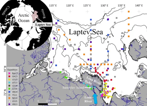
The in situ data presented in this study are compiled from several, mostly unpublished datasets from Russian–German expeditions to the Lena River and Laptev Sea that took place from 2010 to 2017 (Table 1). Sampling locations of this dataset include large parts of the western and central Laptev Sea shelf, coastal regions around the Lena River Delta and channels of the Lena River (Fig. 1).

All ship- and land-based sampling took place during the ice-free period between the end of June and mid-September.

Only one land-based sampling event in the central Lena River Delta took place between the end of May and the end of June, during Lena River peak discharge after the ice break- up. The ship expeditions, which covered offshore shelf wa- ters (NE10, YS11, VB13 and VB14), were conducted on board RVNikolay Evgenov(NE), RVJacob Smirnitsky(YS) and RVViktor Buynitskiy (VB), respectively. For the other ship expeditions, smaller boats were used for sampling in coastal waters or on the Lena River. Water sampling at the research station on Samoylov Island (LD14) was carried out from small boats or from the shore (Fig. 1). Table 1 shows a summary of sampling periods, water types and the sampled parameters of the individual expedition datasets.

2.2 Hydrographic characteristics and sample processing

For each sampling location included in this dataset, vertical profiles of the water column temperature and salinity were measured with a conductivity–temperature–depth (CTD) de- vice (Sontek CastAway CTD for LD14, LD15, LD16, Byk17 and a Seabird 19+for LD10, LD13, NE10, YS11, VB13, VB14 and GA13). In this study, we use the practical salinity unit (psu) to describe salinity. Aboard ships and boats, wa- ter samples were taken using Niskin bottles or an UWITEC water sampler at defined depths. Since this study focuses on improving satellite retrievals, only surface water sam- ples (discrete samples from 2 and 5 m water depth) were in- cluded in the compiled dataset. Based on visual examination of the water column characteristics, we also included sam- ples from 10 m depth wherever a thick homogeneous upper mixed layer was present. During the expedition LD14, wa- ter samples were taken from the shore of Samoylov Island at around 0.5 m depth using 5 L glass bottles.

Water samples for DOC analysis were filtered through a 0.7 µm GF/F filter and acidified with 25 µL HCl Supra- pur (10 M) after sampling. Samples were stored cool and dark for transport. DOC concentrations were measured us- ing high-temperature catalytic oxidation (TOC-VCPH, Shi- madzu). Three measurements of each sample were averaged and after each 10 samples, a blank and a standard (Battle-02, Mauri-09 or Super-05 certified reference material from Na- tional Laboratory for Environmental Testing, Canada) were measured for quality control.

Samples for a_CDOM(λ) analysis were filtered through 0.22 µm Millipore GSWP filters (GA13, LD16, Byk17) or 0.7 µm Whatman GF/F (LD10, YS11, VB13, VB14, LD14, LD15) after sampling. A 100 mL filtrate was stored cool and dark in amber glass bottles until further analysis.aCDOM(λ) was measured with a spectrophotometer (SPECORD 200, Analytik Jena) by measuring the absorbance (A_λ) at 1 nm in- tervals between 200 and 750 nm. Absorption was calculated from the resulting absorbance measurements via

aCDOM(λ)=2.303·A_λ

L , (1)

whereLis the path length (length of cuvette) to calculate the a_CDOM(λ). Fresh Milli-Q water was used as reference. The quartz cuvette length varied depending on the expected ab- sorption in the sampled water (1 or 5 cm for river or coastal waters, 5 or 10 cm for offshore shelf waters). Resulting a_CDOM(λ)spectra were corrected for baseline offsets by sub- tracting the mean absorption between 680 and 700 nm, as- suming zero absorption at>680 nm. We focussed onaCDOM

at 443 nm since most OCRS algorithms use this wavelength to retrieve aCDOM(λ). This wavelength corresponds to one spectral band of most multispectral satellite sensors. Spectral slopes ofaCDOM(λ) were calculated by non-linearly fitting the following equation (Jerlov, 1968; Bricaud et al., 1981):

aCDOM(λ)=aCDOM(λ0)·e^{−S(λ−λ0)}, (2) whereaCDOM(λ0)is the absorption coefficient at reference wavelengthλ0andSis the spectral slope ofaCDOM(λ)for the chosen wavelength range. Spectral slopes ofaCDOM(λ)were calculated fitting Eq. (2) for the individual wavelength ranges (275 to 295 nm for S275–295 and 350 to 500 nm for S350–

500). The DOC specific absorption coefficient atλ=440 nm was calculated witha^∗_CDOM(440)=a_CDOM(440)/DOC.

2.3 Satellite data

In order to monitor spatiotemporal variability of DOC in surface waters and test the applicability of the established DOC–a_CDOM(λ)model from this study, we used OCRS. We applied the DOC–a_CDOM(λ) model to calculate DOC con- centration from satellite-retrieveda_CDOM(λ). For this study, we chose the Medium Resolution Imaging Spectrometer (MERIS) because of its high spectral resolution and spec- troradiometric quality (Delwart et al., 2007). Many OCRS

Table 1.Expedition focus regions, years and season. Mean and standard deviation of hydrographic and DOM parameters are listed. The number of samples between DOC and a_CDOM(443) differs for some expeditions, and “n.a.” indicates that no DOC measurements were made.

Expedition (code) Focus region

Year Season S(psu) DOC (µmol L⁻¹)

a_CDOM(443) (m⁻¹)

S275–295 (nm⁻¹)

S350–500 (nm⁻¹) Lena 2010 (LD10) Coastal 2010 Aug 6.03±6.59 563±156

(n=29)^a

3.39±0.27 (n=9)

0.0152±0.0006 0.0167±0.0019

Transdrift XVIII (NE10)

Central shelf

2010 Sep 23.6±6.6 n.a. 0.66±0.46 (n=107)

0.0196±0.0016 0.0175±0.0028

Transdrift XIX (YS11)

Central shelf

2011 Aug &

Sep

19.6±3.6 239±55 (n=29)

0.75±0.21 (n=26)

0.0193±0.0009 0.0161±0.0129

Lena 2013 (LD13) Lena River 2013 Jul &

Aug

0.01±0.05 695±77 (n=28)^b

3.25±0.6 (n=28)

0.016±0.0007 0.0166±0.0006

Gonçalves-Araujo et al. (2015) (GA 13)

Coastal 2013 Jul &

Aug

14.2±9.4 398±155 (n=59)^d

1.5±0.86 (n=42)^c

0.017±0.0015 0.0181±0.00158

Transdrift XXI (VB13)

Central shelf

2013 Aug &

Sep

22.6±6.9 n.a. 0.71±0.55 (n=19)

0.0201±0.0023 0.0184±0.0017

Lena 2014 (LD14) Lena River 2014 May &

Jun

0.01±0.05 1049±248 (n=50)

5.66±1.85 (n=44)

0.0145±0.001 0.0159±0.0005

Transdrift XXII (VB14)

Central shelf

2014 Sep 28.3±2.9 176±53 (n=46)

0.36±0.19 (n=47)

0.0208±0.0021 0.0196±0.00164

Lena 2015 (LD15) Lena River 2015 Jul &

Sep

0.01±0.05 n.a. 2.66±0.72 (n=12)^e

0.0167±0.0009 0.0166±0.0006

Lena 2016 (LD16) Lena River

& coastal

2016 Aug &

Sep

7.3±9.5 499±164 (n=17)

2.47±1.22 (n=35)

0.0164±0.001 0.0164±0.0014

Bykovsky 2017 (Byk17)

Coastal 2017 Jun &

Jul

1.3±2.2 675±61 (n=22)

2.6±0.69 (n=22)

0.0161±0.0009 0.019±0.0013

ahttps://doi.org/10.1594/PANGAEA.842220.^bhttps://doi.org/10.1594/PANGAEA.844928.^chttps://doi.org/10.1594/PANGAEA.875748.

dhttps://doi.org/10.1594/PANGAEA.842221.^ehttps://doi.org/10.1594/PANGAEA.875754.

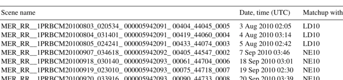
Table 2.List of Medium Resolution Imaging Spectrometer (MERIS) scenes used in this study.

Scene name Date, time (UTC) Matchup with

MER_RR__1PRBCM20100803_020534_ 000005942091_ 00404_44045_0005 3 Aug 2010 02:05 LD10 MER_RR__1PRBCM20100804_031401_ 000005942091_ 00419_44060_0004 4 Aug 2010 03:14 LD10 MER_RR__1PRBCM20100805_024241_ 000005942091_ 00433_44074_0003 5 Aug 2010 02:42 LD10 MER_RR__1PRBCM20100907_034618_ 000005942092_ 00405_44547_0002 7 Sep 2010 03:46 NE10 MER_RR__1PRBCM20100918_030140_ 000005942093_ 00061_44704_0006 18 Sep 2010 03:01 NE10 MER_RR__1PRBCM20100919_023010_ 000005942093_ 00075_44718_0007 19 Sep 2010 02:30 NE10 MER_RR__1PRBCM20100920_033916_ 000005942093_ 00090_44733_0008 20 Sep 2010 03:39 NE10

algorithms were developed specifically for this sensor and are designed for coastal waters. MERIS L1 satellite scenes at reduced resolutions (1 km spatial resolution) were obtained from the MERIS Catalogue and Inventory (MERCI). Scenes with reduced resolution were chosen because of their larger extent and thus better coverage of the in situ data stations.

Furthermore, Hu et al. (2012) reported a better signal-to- noise ratio compared to MERIS full-resolution data and rec- ommended the use of MERIS reduced-resolution data. We

checked all expedition periods for cloud-free MERIS satel- lites scenes but only two expeditions from 2010 (LD10 and NE10 ship expeditions) could be used to evaluate the per- formance of the remote sensing retrieval of the surface wa- ter DOC concentration. During those periods, we identified a few scenes with substantial cloud-free data coverage that were acquired during the 2010 expedition periods. Table 2 lists MERIS scenes used in this study. In order to visu- alize satellite-derived results, we generated mosaic images

B. Juhls et al.: Dissolved organic matter in the Laptev Sea 2697

Figure 1.Map of the Laptev Sea and the Lena River Delta region with sample locations from 11 Russian–German expeditions; upper left map shows the Arctic Ocean and the location of the Laptev Sea on the Russian Arctic shelf. Bathymetry is shown by black contour lines and water depth in metres.

containing the average of the overlap from multiple satel- lite scenes to extend the data coverage between cloud gaps.

To compare in situ with satellite data, we used the median of 3×3 extracted pixel values from each single processed OCRS image. To discuss processes that cause differences be- tween satellite images, we extracted reanalysis surface wind data (four times daily) from the National Centers for Envi- ronmental Prediction (NCEP).

Hieronymi et al. (2017) developed the OLCI (Sentinel- 3 Ocean and Land Colour Instrument) neural network swarm (ONNS) in-water algorithm for the retrieval of OCRS products, among them a_CDOM(440). This algorithm is de- signed for broad concentration ranges of different water con- stituents, including extremely high absorbing waters. The al- gorithm differentiates 13 optical water types (OWTs) and uses specific neural networks (NNs) for each OWT. Every NN is trained for narrow concentration ranges. The values of aCDOM(440) used for the training of the NNs are up 20 m⁻¹. The final product is a weighted sum of all NNs depending on OWT membership. The standard atmospheric correction of ONNS, namely the C2RCC (Brockmann et al., 2016), is applied. ONNS makes use of 11 out of the 21 OLCI bands, including the 400 nm band, which is the only one not de- livered by MERIS. In order to retrieve OCRS products with ONNS from MERIS imagery, a band-adaptation NN algo- rithm is utilized to extrapolate remote sensing reflectance at 400 nm, which is usually provided with an uncertainty<5 % for these waters (Hieronymi, 2019). Note that the ONNS al-

gorithm uses theaCDOM(λ)wavelength of 440 nm, whereas all other algorithms use 443 nm.

Additionally, we tested the following open-source OCRS algorithms: (1) FUB/WeW MERIS Case 2 water properties processor (FUB/WeW) (Schroeder and Schaale, 2005) de- veloped fora_CDOM(443) up to 1 m⁻¹, MERIS Case 2 water algorithm (C2R) (Doerffer and Schiller, 2007) (a_CDOM(443) up to 1 m⁻¹), which is used for the MERIS third repro- cessing of ESA’s distributed products, and the Case 2 Re- gional CoastColour (C2RCC) (Brockmann et al., 2016) with C2RCC (a_CDOM(443) up to 1 m⁻¹)and C2X (a_CDOM(443) up to 60 m⁻¹). All algorithms used in this study use neural networks trained with databases of radiative transfer simu- lations or in situ measurements or both to invert the satel- lite signal into inherent optical water properties such as aCDOM(λ)^satand concentrations such as total suspended sed- iment (TSM). In this study, the atmospheric correction from C2RCC (Brockmann et al., 2016) was used to provide at- mosphere corrected reflectances for the OCRS algorithms (ONNS, C2R, C2RCC and C2X). For the FUB/WeW algo- rithm, the atmospheric correction provided by the FUB/WeW processor (Schroeder and Schaale, 2005) was used.

Functions for satellite retrieval evaluation

In order to evaluate the retrieval of a_CDOM(λ)^sat from the tested OCRS algorithms, we used a number of evaluation pa- rameters suggested by Bailey and Werdell (2006) and Mat-

suoka et al. (2017). Among them, we use the median of satel- lite to in situ ratio (Rt), the semi-interquartile range (SIQR), the median absolute percent error (MPE) and root mean square error (RMSE). The evaluation parameters are defined as follows:

Rt=median Xsat

Xin situ

, (3)

SIQR=Q₃−Q₁

2 , (4)

MPE=median

100·

X_sat−X_{in situ} Xin situ

, (5)

RMSE= v u u u t

N

P

n=1

[Xsat−Xin situ]²

N , (6)

where Xsat andXin situ are the satellite-derived and in situ measuredaCDOM(443), respectively.Q1represents the 25th ratio percentile andQ₃represent the 75th ratio percentile.

3 Results

3.1 Spatial and temporal variability of DOC and CDOM

To examine variability of DOC and CDOM optical proper- ties along the land–ocean continuum of the Lena–Laptev sys- tem, we generated a large dataset that covers spring freshet through late summer from 2010 to 2017 (Table 1). Compared to previously published datasets (Gonçalves-Araujo et al., 2015; Mann et al., 2016; Matsuoka et al., 2012; Walker et al., 2013), this dataset compiles not only samples of one water type but covers river, coastal and offshore waters throughout the most variable portion of the open water season.

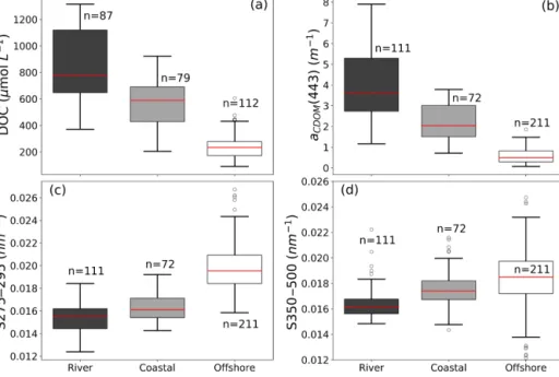
To better understand characteristics of DOC and a_CDOM(λ)in freshwater–marine waters, the compiled dataset was first classified into three water types according to salin- ity: (1) fresh river water with salinities from 0 to 0.2, (2) mesohaline coastal water with salinities from 0.2 to 16 and (3) offshore waters with salinities>16.

Overall, DOC concentrations tended to decrease from river to offshore. The same trend was also observed in aCDOM(443). In river water, DOC concentrations and aCDOM(443) ranged from 370 to 1315 µmol L⁻¹ (me- dian of 779 µmol L⁻¹) and 1.17 to 7.91 m⁻¹ (median of 3.61 m⁻¹), respectively (Fig. 2a and b). DOC concentra- tions and aCDOM(443) in coastal waters ranged from 205 to 923 µmol L⁻¹ (median of 590 µmol L⁻¹) and 0.71 to 3.79 m⁻¹ (median of 2.05 m⁻¹), respectively. Values in offshore water were the least variable of all three water types, with DOC concentrations from 91 to 606 µmol L⁻¹ (median of 234 µmol L⁻¹) and a_CDOM(443) from 0.077 to 1.86 m⁻¹ (median of 0.5 m⁻¹). Generally, observed DOC and a_CDOM(443) values were similar to reported findings

from the Lena River and Laptev Sea regions (Amon et al., 2012; Cauwet and Sidorov, 1996; Gonçalves-Araujo et al., 2015; Heim et al., 2014; Raymond et al., 2007; Stedmon et al., 2011).

The spectral UV slope (S275–295) (Fig. 2c) showed similar maximum and median values for river (max. of 0.0184 nm⁻¹, median of 0.0155 nm⁻¹) and coastal waters (max. of 0.0192 nm⁻¹, median of 0.0161 nm⁻¹). We ob- served the lowest S275–295 in the Lena River water dur- ing the spring freshet at the beginning of June (LD14, Ta- ble 1). Offshore water has significantly higher S275–295 values ranging from 0.0158 to 0.0267 nm⁻¹ (median of 0.195 nm⁻¹). For river and coastal water, S350–500 showed a similar variability to S275–295. The range of offshore wa- ter (S350–500), however, showed substantially higher varia- tion and covered a broad range (Fig. 2d).

In contrast to trends in DOC concentrations and aCDOM(443), aCDOM(λ) spectral slopes in two distinct spectral domains (S275–295 and S350–500) tended to in- crease from river to offshore (Fig. 2). While the spec- tral slopes between river (max. of 0.0184 nm⁻¹, median of 0.0155 nm⁻¹) and coastal waters (max. of 0.0184 nm⁻¹, me- dian of 0.0158 nm⁻¹) were not substantially different, those between the river and offshore were significantly different (p value≤10⁻⁸).

3.2 CDOM absorption characteristics

We compared salinity and aCDOM(443) for the compiled dataset. As in other river-influenced waters, there was a strong linear relationship betweenaCDOM(443) and salinity (r²=0.87,n=283) (Fig. 3), suggesting that physical mix- ing prevails and plays a role in near-conservative behaviour ofa_CDOM(λ). For this analysis, only coastal and offshore wa- ters were included since river water was constant in salin- ity but varied seasonally ina_CDOM(443) (LD14, Table 1). In coastal and offshore waters,a_CDOM(443) decreased gradu- ally with increasing salinity. The observed mixing line is sim- ilar to the reported mixing line for Laptev Sea shelf waters from Heim et al. (2014), which was developed using parts of this compiled dataset (LD10 and YS11). The reported rela- tionship from Matsuoka et al. (2012), however, shows gen- erally loweraCDOM(443) values in waters of the WAO along the salinity gradient. The S350–500 was very variable along the mixing line. However, lowaCDOM(443) along the mix- ing line had high S350–500 and higheraCDOM(443) had low S350–500.

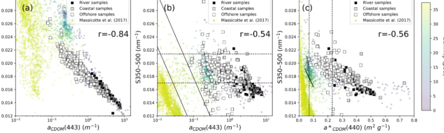
Bulk information, combined use of magnitudes and spec- tral slopes of CDOM absorption are useful for understand- ing sources and/or processes involved in the modification of dissolved organic matter, e.g. Fichot and Benner (2012) and Helms et al. (2008). The strongest correlation was ob- served betweena_CDOM(443) and the UV slope of S275–295 (Fig. 4a, Pearson correlation coefficient (r) of−0.84). Sim- ilar strong correlations were reported by Fichot and Ben-

B. Juhls et al.: Dissolved organic matter in the Laptev Sea 2699

Figure 2.Box plot of(a)DOC concentration,(b)a_CDOM(443), (c)S275–295 and(d)S350–500 for the three water types clustered by salinity (river<0.2, coastal<16, offshore>16); the red line indicates median of each water type.

Figure 3.Relationship betweena_CDOM(443) and salinity (n=283, r²=0.87) for all available water sampled from less than 10 m water depth and a salinity>0.2; colour of data points indicates S350–

500; red dashed line shows the linear fit representing the mixing line between salinity anda_CDOM(443) within this dataset. The solid black line shows the reported mixing line from Heim et al. (2014) and the dashed black line shows the one from Matsuoka et al. (2012) (adapted toa_CDOM(443) using Eq. 2 and a constant slope of 0.018).

ner (2011) between aCDOM(350) and S275–295 for coastal waters of the Beaufort Sea in the WAO. Here, we used a_CDOM(443) to make the findings useful for the OCRS com- munity, which usually retrievesa_CDOMat 443 nm. The spec- tral slope of S350–500 showed moderate correlation with a_CDOM(443) (Fig. 4b,r= −0.54). Furthermore, a high num- ber of S350–500 values were located outside the range of observed S350–500 values for coastal waters of the western Arctic (dashed lines, Fig. 4b).

We observed a moderate correlation betweena_CDOM^∗ (440) and S350–500 (Fig. 4c,r= −0.56). Most samples from this study are located above the a_CDOM^∗ (440) limits of oceanic water reported by Nelson and Siegel (2002), dashed lines in Fig. 4c, indicating that water samples from this study are pri- marily river influenced with higher aromaticity (Granskog et al., 2012; Helms et al., 2008; Weishaar et al., 2003). The reported relationship between a_CDOM^∗ (440) and S350–500 from Matsuoka et al. (2012), solid line in Fig. 4c, deviates strongly in slope of the regression and range ofa_CDOM^∗ (440) values from these data from the fluvial–marine transition zone of the Laptev Sea.

Compared to the global CDOM absorption characteristics from Massicotte et al. (2017) (Fig. 4a to c, coloured circles), samples from this study are within the range of freshwater- influenced samples with lower salinities and clearly differen- tiate from high saline oceanic waters.

3.3 DOC–CDOM relationship

Generally, retrieval of optical water properties and water con- stituents such as DOC from satellite data consists of three steps: (1) atmospheric correction of the top-of-atmosphere radiance to the water-leaving or the in-water reflectance, which is needed as input for the OCRS algorithms, (2) the retrieval ofa_CDOM(λ)^satfrom the atmospherically corrected reflectance received by satellite and (3) ifa_CDOM(λ)^satis re- trieved from OCRS, DOC can be calculated using an in situ DOC versus in situa_CDOM(λ)relationship. The direct valida- tion and evaluation of different atmospheric corrections (1) is beyond the scope of this study. In the following, we present

Figure 4. (a)Relationship betweena_CDOM(443) and S275–295;(b)a_CDOM(443) vs. S350–500 with 95 % confidence intervals of regressions of western Arctic coastal waters (dashed lines) and for western Arctic oceanic water (solid lines) reported by Matsuoka et al. (2011, 2012), (c)a*_CDOM(440) vs. S350–500 with dashed lines representing the borders ofa*_CDOM(440) for oceanic waters reported by Nelson and Siegel (2002), and the solid line shows the reported relationship betweena_CDOM^∗ (440) and S350–500 from Matsuoka et al. (2012). Circles show global data from Massicotte et al. (2017) where colours indicate the salinity.

a new regional DOC–a_CDOM(λ) relationship (3) from our compiled in situ dataset.

We observed a strong relationship between aCDOM(443) and DOC concentration for all water samples including river to marine waters (Fig. 5). Overall, 1 order of magnitude vari- ation in DOC corresponded to more than 2 orders of mag- nitude of variation in aCDOM(443) for this sample set and corresponded to the range from moderately absorbing waters (0.1–1.0 m⁻¹) to highly absorbing waters (>1.0 m⁻¹). After testing different regression models, the best fit was derived with a power function (Eq. 7, red line in Fig. 5):

DOC(µmol L⁻¹)=10^2.525·aCDOM(443)^0.659. (7) The agreement between model and data (r²=0.96,n=227) allowed estimation of DOC by a_CDOM(443) within a 50 % error range. The highest deviations from the fitted line cor- responded to the transition zone between offshore shelf wa- ters and coastal waters (a_CDOM(443) of 0.5–1.5 m⁻¹) and to the very low end of thea_CDOM(443) range (<0.5 m⁻¹). It is noted that the fitting model of this dataset using only offshore or river water samples would result in a lower slope (expo- nent of 0.617 for coastal and offshore water, 0.606 for off- shore water only) in the resulting DOC–aCDOM(443) model.

Including coastal and river samples substantially increased the slope of the fit, which results in higher DOC estimates for highaCDOM(443). The reported relationship from Mann et al. (2016) is similar for high-a_CDOM(443) river water but deviates for low-a_CDOM(443) river water and coastal and off- shore water. The model presented by Matsuoka et al. (2017) (blue line in Fig. 5) has a lower slope and results in the high- est differences for DOC estimation at higha_CDOM(443).

Model coefficients for other selected a_CDOM(λ) wave- lengths are presented in Table A1 (Appendix A). Further- more, the relationship between S275–295 and DOC had

Figure 5. Relationship between a_CDOM(443) and DOC (r²= 0.96). Red line shows the derived model from this dataset. The blue line shows the relationship from Matsuoka et al. (2017) for a pan- Arctic dataset for offshore and coastal waters. The green line shows the relationship for Lena River water from Mann et al. (2016). The filled grey area shows the 50 % error range. Note that the axes are displayed in log scale.

a slightly weaker correlation with DOC (r²=0.92) than a_CDOM(443).

3.4 Satellite-retrieved CDOM

To estimate the surface water DOC concentration with the presented DOC–a_CDOM(λ) model (Eq. 7, Fig. 5) and gen- erate DOC concentration maps for large scales, we need a robust and accurate retrieval ofa_CDOM(λ)^sat.

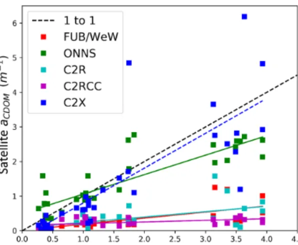
We examined the performance of five OCRS algorithms in terms ofa_CDOM(443)^satretrieval using Eqs. (3) to (6). For this purpose,a_CDOM(443)^satretrievals were compared to in situ data from within 10 d of the satellite retrievals. Our com- parisons showed highly varying results (Figs. 6, B1 in Ap-

B. Juhls et al.: Dissolved organic matter in the Laptev Sea 2701

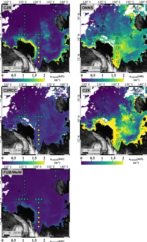
Figure 6.Surface watera_CDOM(λ)^satfrom MERIS mosaic from five scenes from September 2010 (scenes listed in Table 2) for all tested OCRS algorithms (C2R, ONNS, C2RCC, C2X, FUB/WeW). Squares show in situ a_CDOM(443) (a_CDOM(440) for ONNS) with colours according to the same colour scale as satellite data.

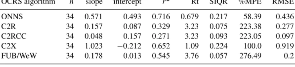
Table 3.Performance of tested OCRS algorithms for a_CDOM(λ)^satwith in situa_CDOM(443) ora_CDOM(440). Note that not all OCRS algorithms are developed for the highly absorbing waters (higha_CDOM(λ)) found in the Arctic coastal region.

OCRS algorithm n slope intercept r² Rt SIQR %MPE RMSE

ONNS 34 0.571 0.493 0.716 0.679 0.217 58.39 0.436

C2R 34 0.157 0.087 0.329 3.23 0.075 223.38 0.277

C2RCC 34 0.048 0.157 0.271 3.23 0.093 223.05 0.097

C2X 34 1.023 −0.212 0.652 1.09 0.224 100.0 0.919

FUB/WeW 34 0.178 0.013 0.545 3.76 0.057 276.49 0.2

pendix B, Table 3) and strong under- or overestimation of aCDOM(λ)^sat. Particularly in turbulent coastal waters, com- parison of aCDOM(443)^sat with in situ aCDOM(443) is chal- lenging, given the fact that the magnitude of CDOM ab- sorption can vary greatly over a short time for the loca- tion of a given pixel. ONNS-deriveda_CDOM(λ)^satperformed best (r²=0.716, Rt of 0.679, SIQR of 0.217, %MPE of 58.39, RMSE of 0.436). The C2X algorithm performed sim- ilarly with a lowerr²(0.65) and substantially higher %MPE (100.0) and RMSE (0.919). In addition to the comparison with in situ data, we evaluated the plausibility of the result- ing spatial distributions and observed extremely high C2X- derived aCDOM(443)^sat values in the Lena River mouth (up to 10 m⁻¹). Such values ofaCDOM(443) were not confirmed by any reported in situ data. ONNS-derived aCDOM(443)^sat showed values which are in the range of in situ observed aCDOM(443). Other algorithms show clear underestimations of aCDOM(443)^sat compared to in situ data (Fig. B1). Thus, ONNS was the only algorithm that produceda_CDOM(λ)val- ues in a similar range to in situ measureda_CDOM(440).

3.5 Surface water DOC concentrations in coastal waters of the Laptev Sea

Using the presented DOC–a_CDOM(λ)model, we generated satellite-derived images of surface water DOC concentra- tions for the Lena–Laptev region. All scenes were processed with the ONNS algorithm, anda_CDOM(440) was averaged for each mosaic. DOC concentrations for two mosaics (Fig. 7b, d) were calculated by using the adapted model from Eq. (7) with coefficients for aCDOM(440) instead of aCDOM(443).

The mean time difference between the two mosaics is 31 d.

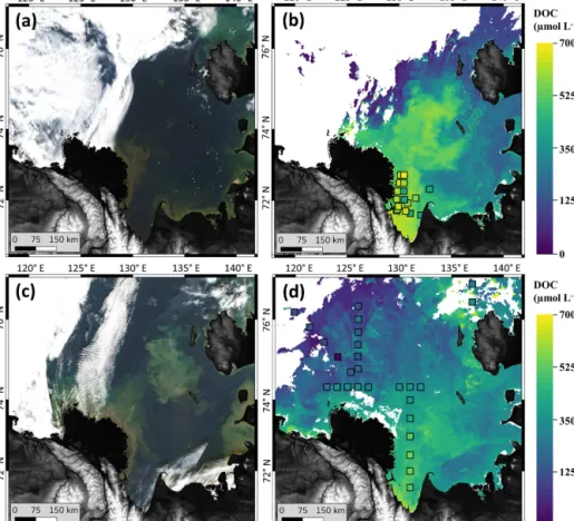
The DOC mosaic from early August 2010 (Fig. 7b) shows high DOC concentrations over large areas in the eastern Laptev Sea. Concentrations (>600 µmol L⁻¹) were highest in Buor-Khaya Bay east of the Lena River Delta where the Lena River exports most of its water. The plume of the Lena River with high DOC concentrations (∼500 µmol L⁻¹) had propagated northeastward in this scene. The DOC mosaic from September 2010 (Fig. 7d) shows generally lower DOC concentrations compared to the earlier scene. Highest con- centrations were found in the coastal areas in Buor-Khaya Bay (east of the Lena River Delta) and around the Olenek River Delta (west of the Lena River Delta). While ONNS per-

forms well in river-influenced waters, we note that DOC con- centrations at the northern edge can be influenced by cloud masking (patches of high DOC concentrations shown in the northeast corner of Fig. 7d).

Both quasi-true colour satellite images (Fig. 7a, c) show sediment-rich, strongly backscattering waters around the Lena River Delta resulting from fluvial transport. In the satel- lite image from 7 September 2010 (Fig. 7c), there is also a large strongly backscattering area in the eastern Laptev Sea, where resuspension events in shallow water (5–10 m, Fig. 1) occurred between both acquisition periods. These resuspen- sion events are not visible in the calculated DOC concentra- tion maps on the right (Fig. 7d).

In situ DOC vs. remotely sensed DOC

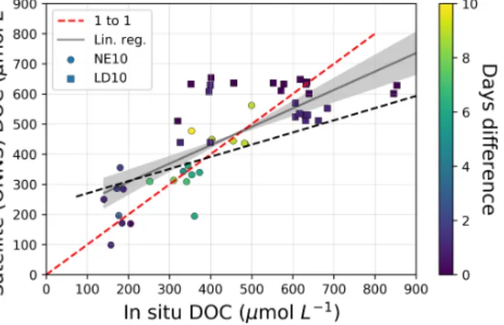
To evaluate the satellite-retrieved DOC concentrations, we compared in situ and ONNS-retrieved DOC concentrations (Fig. 8) using the presented DOC–aCDOM(λ)model (Eq. 7) and investigated the plausibility of the DOC value ranges and the derived spatial patterns (Fig. 7b, c). This evaluation re- vealed a moderate performance (r²=0.53, slope of 0.61) (Fig. 8) despite several days’ difference in sampling times between satellite and in situ sampling. The use of MERIS full-resolution data revealed a slightly better performance (r²=0.68, slope of 0.77). However, we preferred the use of reduced-resolution data due to the reported better qual- ity (Hu et al., 2012). This comparison constitutes an eval- uation and not a direct validation of the method. The latter is hampered by the lack of matching data and the time off- sets between satellite acquisition and in situ sampling dates.

The DOC–aCDOM(λ)model presented in this study improved satellite-derived estimates of DOC concentration compared to estimates using the DOC–aCDOM(λ)relationship reported by Matsuoka et al. (2017) (r²=0.46, Fig. 8).

To spare in situ data for this performance test, data from LD10 were not used to develop the DOC–a_CDOM(λ)model (Eq. 7). The DOC concentrations for NE10 were calculated from in situa_CDOM(443) measurements using Eq. (7), since no in situ DOC measurements were taken on NE10. These in situ DOC concentrations are therefore not independent but were derived from the DOC–a_CDOM(443) relationship for the entire dataset. However, samples from NE10 were not used for the development of the DOC–a_CDOM(λ) relation-

B. Juhls et al.: Dissolved organic matter in the Laptev Sea 2703

Figure 7. (a)Quasi-true colour image from 5 August 2010.(b)Surface water ONNS-DOC concentration from satellite mosaics from 3 to 5 August 2010.(c)Quasi-true colour image from 7 September 2010.(d)Surface water ONNS-DOC concentration from satellite mosaics from 7 September 2010 and 18 to 20 September 2010. Squares in panels(b)and(d)indicate in situ concentrations with the same colour scale as satellite data.

ship since in situ DOC was missing. We use the data to test the DOC retrieval for a wide range of concentrations. Fur- ther validation of the DOC retrieval will require additional in situ datasets collected simultaneously with cloud-free, open- water remote sensing acquisitions by using the MERIS suc- cessor OLCI.

4 Discussion

4.1 Sources and modification of DOM in the fluvial–marine transition

Our results showed that aCDOM(443) decreases as a func- tion of salinity (Fig. 3), indicating that river water is the main source of CDOM on the Laptev Sea shelf waters and in coastal waters and thus that most CDOM is of terrige- nous origin. Despite the tight relationship, some data points deviated from the mixing line in the salinity range from 2 to 24. Deviations from the mixing line can result from combined physical, chemical and biological processes that modify CDOM optical properties (Asmala et al., 2014; Mat- suoka et al., 2015, 2017). Helms et al. (2008) and Matsuoka

et al. (2012) suggested that higheraCDOM(443) and lower S350–500 can be used as a proxy indicating that microbial degradation is more important than photodegradation. In- deed, we observed higheraCDOM(443) associated with lower S350–500 within a similar salinity range (Fig. 3), pointing towards stronger microbial degradation than photodegrada- tion.

Flocculation can also modify CDOM optical properties by removing larger molecules once the river water encounters saline water. However, given the fact that this process oc- curs at low salinities (0 to 3) (Asmala et al., 2014), floccula- tion alone cannot explain the deviation ofa_CDOM(443) values apart from the mixing line.

S275–295 was strongly correlated with a_CDOM(443) (Fig. 4a), which is mainly associated with the high-content lignin chromophores in our samples (Fichot et al., 2013) and is partly explained by the long exposure of DOM to solar radiation and the resulting photodegradation (Hansen et al., 2016; Helms et al., 2008). Lena River water shows high lignin content and higher proportion of syringyl and vanylphenols relative to p-hydroxyphenols (Amon et al., 2012). Benner and Kaiser (2011) showed that this could

Figure 8. Comparison of in situ DOC and ONNS-derived DOC.

The dark grey line shows a linear regression (r²=0.53, slope of 0.61, n=50). The grey area represents the 95 % confidence in- terval. The red line indicates 1:1 correspondence. Day difference (symbol colour) shows the temporal offset between the satellite scene and in situ water sampling. The dashed black line shows the satellite DOC concentration calculated by using the DOC–

a_CDOM(443) relationship from Matsuoka et al. (2017).

make the DOM more subject to photodegradation, which might supports why such a high correlation was observed.

Compared to the strong relationship between S275–295 and aCDOM(443), a moderate correlation was observed for S350–500 versus aCDOM(443) relationship (Fig. 4b), sug- gesting different degradation mechanisms were involved dur- ing the transition from river to coastal and offshore waters.

Here, we use S350–500, which is often used in the OCRS community (Babin et al., 2003; Matsuoka et al., 2011, 2012), instead of S350–400, which is the wavelength range sug- gested by Helms et al. (2008). Note that the correlation be- tween S350–500 and S350–400 is very high (r=0.98), and thus both slopes can be used. The mean river endmember value of S350–500 at zero salinity was 0.0163 nm⁻¹. This value tends to be lower in the EAO (including Lena River mouth) than in the WAO (Matsuoka et al., 2017; Stedmon et al., 2011). The higher a_CDOM(443) associated with the lower spectral slope observed in our river and coastal wa- ters suggested more aromaticity in waters obtained from the Lena–Laptev region (Stedmon et al., 2011). This was further demonstrated by our highera_CDOM^∗ (443) (Fig. 4c).

The S350–500 versusaCDOM(443) relationship showed a moderate but significant negative correlation and most sam- ples were within a terrestrial range (dashed lines, Fig. 4b).

The fact that no samples were within the reported ranges of photodegradation for oceanic waters (solid lines, Fig. 4b) suggests that CDOM in coastal waters of the Laptev Sea would have been highly influenced by terrestrial inputs but with the least photodegradation effect compared to that in oceanic waters (Matsuoka et al., 2015, 2017). It is likely that high turbidity and thus less transparent water of coastal re-

gions in the Laptev Sea protects DOM from photodegrada- tion. Data points outside of the ranges might indicate either microbial degradation and/or sea-ice melt (Matsuoka et al., 2017). Given the only minor influence of ice melt waters during most of our field campaigns, microbial degradation is more likely for some of our samples, which is consistent with our explanation for deviated samples shown in Fig. 3.

The difference in optical properties ofa_CDOM(λ)observed between EAO and WAO is possibly caused by geological dif- ference rather than climatic influences (Gordeev et al., 1996).

This is partly supported by the chemical characterization of lignin phenols (Amon et al., 2012). Our results showed specificity of optical properties in the Lena River and Laptev Sea and underline the necessity of discussing spectral opti- cal properties whenaCDOM(443) and DOC concentration are estimated in this region.

4.2 Linking CDOM absorption to dissolved organic carbon concentration

Previous reported DOC–a_CDOM(λ) models such as Walker et al. (2013), Örek et al. (2013) and Mann et al. (2016) for Arctic rivers, Matsuoka et al. (2012) for WAO and Gonçalves-Araujo et al. (2015) for coastal waters are re- stricted in their use to the water type of samples. Our pre- sented DOC–a_CDOM(λ)relationship improves reported mod- els from Mann et al. (2016) and Matsuoka et al. (2017) for the estimation of DOC fromaCDOM(443) in DOC-rich waters in transition zones of river and seawater of the Lena–Laptev region. Matsuoka et al. (2017) provided satellite-retrieved DOC concentration maps for coastal waters of the Lena River Delta region, retrieved with a DOC–a_CDOM(443) re- lationship developed using a pan-Arctic in situ dataset. How- ever, the retrieved DOC concentrations were likely underes- timated compared to in situ measurements in the coastal re- gions of the Laptev Sea presented in this study. In coastal or a_CDOM(443)-rich, river-influenced water, the difference be- tween the two relationships is expected to be highest. Apply- ing the Matsuoka et al. (2017) relationship toa_CDOM(443)- rich waters outside its validity ranges (>3.3 m⁻¹) would re- sult in underestimation of DOC compared to the relationship presented in this study. Taking mean Lena RiveraCDOM(443) of 4.1 m⁻¹, which is similar to the highestaCDOM(443) val- ues in coastal waters, the difference in modelled DOC con- centration between both relationships is 186.8 µmol L⁻¹. The main reason for this underestimation is likely the lack of near-coastal and river water samples with high DOC for the development of their relationship. This hypothesis was con- firmed by testing the relationship of our dataset by removing coastal and river water. This decreased the slope of the fit- ting model and led to an underestimation of DOC in coastal and river waters (without coastal and river water: slope of 0.617). The slope of the reported fitting model from Mat- suoka et al. (2017) is lower (0.448), compared to the fitting model from this study (all samples: slope of 0.664). This dif-

B. Juhls et al.: Dissolved organic matter in the Laptev Sea 2705 ference highlights the importance of using a broad concen-

tration range to develop such relationships.

The broad concentration range of the relationship pre- sented here permits the generation of remotely sensed sur- face DOC concentration maps of the Laptev Sea across the fluvial–marine transition zone usinga_CDOM(443). The appli- cability of this relationship for other Arctic fluvial–marine transition regions (e.g. Yenisei, Ob, Kolyma, Mackenzie) is untested and the relationship may need to be extended with regionally specific data.

Previous studies usinga_CDOM(443) often focused on dif- ferent wavelengths for aCDOM(λ). The shape of the DOC–

aCDOM(λ)relationship is strongly dependent on the chosen aCDOM(λ)wavelength, whereas DOC–aCDOM(350) shows a linear relationship,aCDOM(443) can be better described with a power function (see Eq. 7). Table A1 provides coefficients for selectedaCDOM(λ)wavelengths. We encourage the data publication of all available wavelengths foraCDOM(λ)mea- surements in future studies to enable direct comparisons be- tween studies and regions.

ONNS-derived DOC

The evaluation of ONNS-derived a_CDOM(λ)^sat performed best when tested with in situ data (Table 3). Thus, we se- lected the ONNS-derived a_CDOM(440)^sat to calculate DOC concentration based on the Eq. (7). The evaluation of ONNS- derived DOC concentrations showed moderate performance (r²=0.53). We suggest that the only moderate agreement likely results from rapid movement of near-coastal water fronts. Fluvial–marine transition zones, as in this study area, are characterized by rapidly moving water fronts with large variations in DOC concentration. A spatial shift of a plume between in situ sampling and the satellite acquisition can cause large errors in the match-up performance. All samples from LD10 expedition are located in the near-coastal areas east of the Lena River Delta where rapid movements of water fronts are likely. This could partly explain deviations com- paring in situ measurements and the satellite-derived DOC at a given pixel. Taking this into account, the observed agree- ment shows an adequate retrieval of DOC by satellite using the OCRS ONNS algorithm.

Using satellite-retrieved surface water DOC concentration maps (Fig. 7b, d), we demonstrated rapid changes in DOC concentrations in the Laptev over 1 month in late summer.

The rapid DOC decrease can result from a combination of vertical mixing, dilution and microbial and photodegradation of the organic material in the surface water (Fichot et al., 2013; Holmes et al., 2008; Mann et al., 2012). OCRS could potentially be used to monitor the rapid removal of DOM by degradation from surface waters on Arctic shelves.

4.3 OCRS algorithms in shallow Arctic fluvial–marine transition zones

We observed specific problems ofa_CDOM(λ)^satretrievals for optically complex shallow shelf waters using different OCRS algorithms. The retrieveda_CDOM(λ)^satin shallow waters of- ten shows a co-variation with high TSM, which is a re- sult of high particle backscatter in the water such as sed- iments or some phytoplankton types. In our study, we ob- served that most OCRS algorithms show a strong coupling ofa_CDOM(λ)^satand TSM in all areas of high sediment con- centration (compare Figs. 7 and 9b).

Our study area, the Laptev Sea shelf, is characterized by extremely shallow waters with frequent resuspension of sed- iments from the seafloor, for example, during storm events.

In the Lena River plume, close to the river mouth, where large amounts of TSM and organic matter are transported to the Arctic Ocean, we expect DOC and TSM to co-vary.

Once exported by the Lena River, most particles quickly set- tle to the seafloor, whereas DOM concentration gradually de- creases with increasing physical mixing and ongoing degra- dation. In offshore resuspension areas with very high TSM concentration, DOC and TSM do not necessarily co-vary.

Large amounts of terrigenous organic matter can be miner- alized on short timescales (about 50 % within a year; Kaiser et al., 2017) and strongly degraded when deposited in sedi- ments (Bröder et al., 2016, 2019; Brüchert et al., 2018).

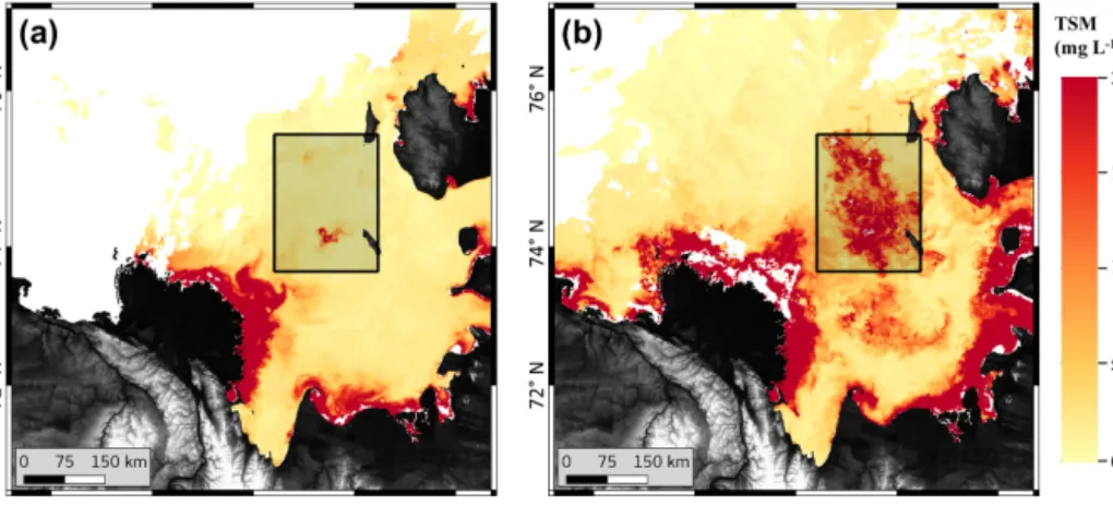
We observe a strong increase of TSM concentrations in the eastern Laptev Sea in September (Fig. 9b) compared to Au- gust (Fig. 9a), which is likely caused by differences in wind speed and resulting wave energy leading to resuspension.

During acquisitions in August, wind speeds were very low (NCEP reanalysis mean surface wind speed of 2.06 m s⁻¹for 75^◦N and 132.5^◦E from 1 to 5 August 2010), whereas in September winds were stronger (NCEP reanalysis mean sur- face wind speed of 6.54 m s⁻¹for 75^◦N and 132.5^◦E from 4 to 20 September 2010). A high TSM concentration in the near-coastal regions around the Lena River Delta, caused by the sediment export by the Lena River, is similar in both mo- saics.

The evaluation of OCRS algorithms with in situ data showed the generally good performance of the ONNS and the C2X algorithms (Table 3). However, shallow resuspension areas are not covered by in situ measurements. Thus, the per- formance of OCRS algorithms cannot be tested in these ar- eas. Whereas the C2X algorithm derives highaCDOM(443) in the resuspension areas in the eastern Laptev Sea, the ONNS algorithm derives loweraCDOM(440) (Fig. 6).

Including all pixels of each scene (Fig. 6), the ONNS- derived a_CDOM(440) does not show a linear relationship with TSM concentration (Fig. 10a). However, using only pixels proximal to the Lena River Delta, we observe a correlation (r=0.68), which is caused by the co-variation of TSM and a_CDOM(440) in the river plume. The C2X- derived a_CDOM(443) shows a linear relationship between

Figure 9.ONNS-derived TSM concentration for satellite mosaics from(a)August 2010 and(b)September 2010. The shallow water area is highlighted by the black square.

Figure 10.Relationship between(a)ONNS-retrieveda_CDOM(440) and TSM concentration and (b) C2X-retrieveda_CDOM(440) and TSM concentration for the MERIS scene from 7 September 2010.

The relationship, using other scenes from September, does not vary significantly (18 September 2010: ONNSr²=0.22 and C2Xr²= 0.55, 19 September 2010: ONNSr²=0.23 and C2Xr²=0.67, 20 September 2010: ONNSr²=0.03 and C2Xr²=0.66).

a_CDOM(443) and TSM (r=0.79). The correlation regimes of thea_CDOM(443) and TSM from river mouth regions and resuspension areas are visible (Fig. 10b). Thus, we show that C2X-derived a_CDOM(443) might vary with TSM. Fur- ther confirmation of these satellite-based observations with in situ data is currently not possible due to a lack of in situ data in shallow areas. A partial independence between ONNS-retrievedaCDOM(440) and TSM is of high importance in shallow Arctic shelf waters, such as the Laptev Sea. Us- ing C2X algorithm, resuspension events would result in erro- neous estimation ofaCDOM(443).

Furthermore, the C2X-derived TSM concentration is sub- stantially higher compared to TSM concentration derived by ONNS (Fig. 10). Örek et al. (2013) and Heim et al. (2014) report TSM concentrations between 10 and 70 mg L⁻¹ for Lena River water and up to 18 mg L⁻¹in coastal water near the Lena River Delta measured in situ in August 2010. These values are similar to TSM concentrations derived by the

ONNS algorithms but lower than C2X algorithm TSM. Con- sidering overestimation of C2X-derived a_CDOM(443) and TSM compared to in situ data, the use of neural networks trained for a broad range of constituent concentration likely leads to inaccurate results. The combination of neural net- works with narrow concentration ranges and a classification into distinct water types (results of classification shown in Fig. C1, Appendix C), as used in the ONNS algorithm, pro- vides more robust and accurate results in regions with a broad range of water types.

5 Conclusion

In this study, we demonstrate sources and modification of DOM by analysingaCDOM(λ)characteristics in the fluvial–

marine transition zone where the Lena River meets the Laptev Sea. Our results suggest that thea_CDOM(λ) spectral slope of S350–500 could be useful to identify and distinguish processes that degrade DOM at this transition. Comparisons of a_CDOM(λ) characteristics from this study with reported values from a global dataset and western Arctic waters iden- tify DOM sources as primarily terrigenous.

We demonstrate the strength of a large in situ dataset that covers multiple water types for deriving the relation- ship between the optical DOM properties and DOC con- centration in surface water of the Laptev Sea and Lena Delta region. The broad range of DOC concentrations and aCDOM(443) from river, coastal and offshore water used to develop this model enables the accurate estimation of DOC byaCDOM(λ) in the transition zone between river and sea- water. Comparing satellite-retrieveda_CDOM(440), using the OCRS ONNS algorithm, and in situ a_CDOM(440) demon- strates the performance of the algorithm for these optically complex waters. DOC concentrations calculated from satel- lite data moderately agreed with in situ DOC measurements (r²=0.53), demonstrating the applicability of the DOC–

a_CDOM(λ) relationship from our compiled dataset. ONNS-

B. Juhls et al.: Dissolved organic matter in the Laptev Sea 2707 derivedaCDOM(440) was found to be independent of the sus-

pended sediment concentration. Thus, resuspension events and resulting sediment-rich backscattering waters seem to have little or no influence on the accuracy of ONNS-derived a_CDOM(440).

The Arctic coastal waters of the Laptev Sea are a key re- gion for the fate of terrestrial DOM and can be monitored synoptically using optical remote sensing with a reasonable accuracy. MERIS-retrieved DOC concentrations presented in this study provide a detailed picture of the spatial distribution of the DOC-rich Lena River water on the Laptev Sea shelf and indicate the rapid changes in the magnitude of DOC con- centrations in the surface waters within short time periods.

If cloud distribution allows, optical remote sensing provides data of high spatial and temporal resolution to track freshwa- ter pathways in the Arctic Ocean, which are of high interest to the oceanographic community.

Data availability. Data have been made available through PAN- GAEA: https://doi.pangaea.de/10.1594/PANGAEA.898813 (Juhls et al., 2019).

Appendix A

The regression between DOC andaCDOM(λ)was performed for a number of selected wavelengths (λ)to enable compar- isons with other studies. Table A1 shows regression coeffi- cients dependent on wavelengths.

Table A1.Coefficients selected wavelengths fora_CDOM(λ)using the equationb·aCDOM(λ)^c.

λofa_CDOM(λ) b c

254 20.9462548427 0.8483590018983822 350 97.4272121688 0.7260394049434391

375 136.577758485 0.715114349676763

440 322.902097112 0.6667788739998305 443 333.695151626 0.6640204313768572

Appendix B

Performance of all tested OCRS algorithms is shown in Fig. B1. Whereas ONNS and C2X provide reasonable re- sults close to the 1:1 line compared to in situ data, other algorithms (C2R, C2RCC, FUB/WeW) underestimate a_CDOM(λ)^satstrongly.

Figure B1.Comparison of in situa_CDOM(443) ora_CDOM(440) witha_CDOM(λ)^satfrom different OCRS algorithms.

B. Juhls et al.: Dissolved organic matter in the Laptev Sea 2709 Appendix C

The percentage membership of each pixel is then used to cal- culate a weighted sum of different neural networks trained for different OWTs. Figure C1 shows the OWTs of the pro- cessed scenes from Figs. 6 and 7. It is visible that Lena River plume in the coastal waters was classified as OWT 1 (see

“1” in Fig. C1) which indicates optically complex, extreme absorbing and high scattering water. The plume between the Lena Delta and the New Siberian Island is characterized by OWT 5 (see “2” in Fig. C1a, b), which indicated a mixture of high-absorbing and scattering waters. The Lena River wa- ter plume with generally Case 2 optically complex waters is sharply delineated to the west, where different water types occur (see “3” in Fig. C1a). Waters west of this plume were classified as OWT 11, displaying Case 1 waters (generally optically deep waters) with a small fraction of absorbing wa- ters.

Figure C1.Optical water types from ONNS fuzzy logic classification for(a)average of 3–5 August 2010 and(b)average of 7 and 18–

20 September 2010.