Microwave and Optical Remote Sensing Data
Mapping of Land Use / Land Cover, Crop - Type, and Crop Traits
I n a u g u r a l - D i s s e r t a t i o n zur
Erlangung des Doktorgrades
der Mathematisch-Naturwissenschaftlichen Fakultät
der Universität zu Köln
vorgelegt von Christoph Hütt aus Ludwigshafen
Köln
2019
Berichterstatter: Prof. Dr. Georg Bareth Prof. Dr. Karl Schneider
Tag der letzten mündlichen Prüfung: 8. Mai 2019
Abstract
Humanity has changed the earth’s surface to a dramatic extent. This is especially true for the area used for agricultural production. Against the background of a growing world population and the associated increased demand for food, it is precisely this area that will become even more important in the future. In order not to have to allocate even more land to agricultural use, optimization and intensification is the only way out of the dilemma. In this context, precise Geoin- formation of the agriculturally used area is of central importance. It is utilized for improving land use, producing yield forecasts for more stable food security, and optimizing agricultural management. Rapid developments in the field of satellite-based remote sensing sensors make it possible to monitor agricultural areas with increased spatial, spectral and temporal resolution. However, to retrieve the needed information from this data, new methods are needed. Furthermore, the quality of the data has to be verified. Only then can the presented geodata help to grow crops more sustainably and more efficiently.
This thesis develops new approaches for monitoring agricultural areas using the technology of microwave remote sensing in combination with optical remote sensing and existing geodata. It is framed by the overall objective to obtain knowledge on how this combination of data can provide the necessary geoinformation for land use studies, precision farming, and agricultural monitoring systems. Hundreds of remote sensing images from more than eight different satellites were analyzed in six research studies from two different Areas of Interest (AOIs).
The studies guide through various spatial scales. First, the general
Land Use / Land Cover (LULC) on a regional level in a multi-sensor
scenario is derived, evaluating different sensor combinations of varying
resolutions. Next, an innovative method is proposed, through which the high geometric accuracy of radar-imaging satellite sensors is exploited to update the spatial accuracy of any external geodata of lower spatial accuracy. Such external data is then used in the next two studies, which focus on cost-effective crop type mapping using Synthetic Aperture Radar (SAR) images. The resulting enhanced LULC maps present the annually changing crop types of the region alongside external, official geoinformation that is not retrievable from remote sensing sensors. The last two research studies deal with a single maize field, on which high resolution optical WorldView-2 images and experimental bistatic SAR observations from TanDEM-X are assessed and combined with ground measurements.
As a result, this thesis shows that, depending on the AOI and the application, different resolution demands need to be fulfilled before LULC, crop type, and crop traits mapping can be performed with adequate accuracy. The spatial resolution needs to be adapted to the particularities of the AOI. Evaluation of the sensors showed that SAR sensors proved beneficial for the study objective. Processing the SAR images is complicated, and the images are unintuitive at first sight. However, the advantage of SAR sensors is that they work even in cloudy conditions. This results in an increased temporal resolution, which is particularly important for monitoring the highly dynamic agricultural area. Furthermore, the high geometric accuracy of the SAR images proved ideal for implementing the Multi-Data Approach (MDA). Thus information-rich external geodata could be used to lower the remote sensing resolution needs, improve the accuracy of the LULC-maps, and to provide enhanced LULC-maps. The first study of the maize field demonstrates the potential of the WorldView-2 data in predicting in-field biomass variations, and its increased accuracy when fused with plant height measurements. The second study shows the potential of the TanDEM-X Constellation (TDM) to retrieve plant height from space.
LULC, crop type and information on the spatial distribution of
biomass can thus be derived efficiently and with high accuracy from
the combination of SAR, optical satellites and external geodata. The
shown analyses for acquiring such geoinformation represent a high
potential for helping to solve the future challenges of agricultural
production.
Zusammenfassung
Die Menschheit hat die Erdoberfläche in dramatischem Maße ver- ändert. Dies gilt insbesondere für die durch landwirtschaftliche Pro- duktion genutzte Fläche. Vor dem Hintergrund einer wachsenden Weltbevölkerung und dem damit verbundenen erhöhten Bedarf nach Nahrungsmitteln werden gerade diese Gebiete in Zukunft weiter an Bedeutung zunehmen. Um nicht noch mehr Flächen für die land- wirtschaftliche Nutzung bereitstellen zu müssen, ist Optimierung und Intensivierung der einzige Ausweg aus dem Dilemma. Von zen- traler Bedeutung sind dabei Geoinformationen der landwirtschaft- lich genutzten Fläche. Sie werden eingesetzt zur Verbesserung der Landnutzung, zur Erstellung von Ertragsprognosen für eine stabilere Ernährungssicherheit und zur Optimierung des Agrarmanagements.
Rasante Entwicklungen auf dem Gebiet der satellitengestützten Fern- erkundungssensoren ermöglichen es, landwirtschaftliche Flächen mit erhöhter spektraler, räumlicher und zeitlicher Auflösung abzubilden.
Um jedoch die benötigten Informationen aus den Daten zu gewinnen, bedarf es neuer Methoden. Zusätzlich muss die Qualität der Daten verifiziert werden, nur dann können die präsentierten Geodaten da- zu beitragen, den Nutzpflanzenanbau nachhaltiger und effizienter zu gestalten.
In dieser Arbeit werden neue Ansätze für die Beobachtung land-
wirtschaftlicher Flächen entwickelt. Dazu wird die Technologie der
satellitengestützten Synthetic Aperture Radar (SAR) Mikrowellenfern-
erkundung mit optischer Satelittenfernerkundung und bestehenden
Geodaten kombiniert. Das übergeordnete Ziel der Arbeit ist es, Er-
kenntnisse darüber zu gewinnen, wie diese Datenkombination die
notwendigen Geoinformationen für Landnutzungsstudien, Präzisions-
landwirtschaft und landwirtschaftliche Überwachungssysteme liefern
kann. Hunderte Fernerkundungsbilder von mehr als acht unterschied- lichen Satellitensystemen wurden in sechs Forschungsstudien aus zwei verschiedenen Untersuchungsgebieten analysiert. Die Studien leiten durch die verschiedenen berücksichtigten räumlichen Skalen. Zu Be- ginn wird die allgemeine Landnutzung auf regionaler Ebene in einem Multisensor-Szenario abgeleitet, dabei werden verschiedene Sensorkom- binationen mit unterschiedlichen Auflösungen bewertet. Als nächstes wird ein innovatives Verfahren vorgestellt, durch das die hohe geome- trische Genauigkeit der SAR-Satelliten genutzt wird, um die räumliche Lagegenauigkeit externer Geodaten mit geringerer Genauigkeit zu verbessern. Solche externen Geodaten sind ein Fokus der nächsten beiden Studien, die kosteneffiziente Feldfruchtkartierung mithilfe von SAR-Bildern demonstrieren. Die daraus resultierenden verbesserten Landnutzungskarten zeigen die jährlich wechselnden Feldfrüchte der Region in Kombination mit externen, offiziellen Geoinformationen, die normalerweise nicht von Fernerkundungssensoren ermittelt werden können. Die letzten beiden Forschungsarbeiten befassen sich mit einem Maisfeld, auf dem hochauflösende optische WorldView-2-Bilder und experimentelle bistatische SAR Beobachtungen von TanDEM-X, mit Bodenmessungen bewertet und kombiniert werden.
Die Ergebnisse der Arbeit zeigen, dass je nach Untersuchungsge-
biet unterschiedliche Auflösungsanforderungen erfüllt sein müssen,
bevor Landnutzung, Feldfrüchte und Pflanzeneigenschaften mit aus-
reichender Genauigkeit kartiert werden können. Es zeigte sich, dass
die räumliche Auflösung an die Besonderheiten der Untersuchungs-
region angepasst werden muss. In einer weiteren Sensorbewertung
erwiesen sich die eingesetzten SAR Sensoren als vorteilhaft für das
Studienziel. Obwohl die Bearbeitung der SAR Bilder kompliziert
ist, und die Bilder auf den ersten Blick ungewohnt wirken, wurde
der Vorteil der SAR Sensoren deutlich: auch bei bewölktem Himmel
werden Daten geliefert. Diese Eigenschaft führt zu einer erhöhten
zeitlichen Auflösung, die sich als essentiell für die Überwachung der
hochdynamischen landwirtschaftlichen Flächen herausstellte. Darüber
hinaus erwies sich die hohe geometrische Genauigkeit der SAR Bilder
als ideal für die Implementierung des Multi-Data Approach (MDA).
Somit konnten informationsreiche externe Geodaten verwendet wer- den, um die Auflösungsanforderungen an die Fernerkundungsdaten zu senken, die Genauigkeit der Landnutzungskarten zu verbessern und um verbesserte, mit externen Geoinformationen angereicherte Landnutzungskarten zu erstellen. Die erste der beiden Maisfeldstudien zeigte das Potenzial des optischen Satellitensystems WorldView-2 für die Detektion von Biomassevariationen innerhalb eines Feldes und eine erhöhte Genauigkeit der Biomasseschätzung bei der Hinzunahme von Pflanzenhöhenmessungen. Die zweite Maisfeldstudie demonstrierte das Potenzial der TanDEM-X Konstellation, die Pflanzenhöhe auch aus dem Weltraum zu messen.
Landnutzung, Feldfruchtkartierungen und Informationen über die
räumliche Verteilung von Biomasse lassen sich also aus der Kombi-
nation von SAR und optischen Satelliten und externen Geodaten
effizient und mit hoher Genauigkeit ableiten. Die gezeigten Analysen
zur Gewinnung der Geoinformation stellen ein großes Potential dar
und können helfen, die zukünftigen Herausforderungen landwirtschaft-
licher Produktion zu meistern.
Acknowledgements
I owe my sincere gratitude to Prof. Dr. Bareth, who supervised this dissertation. He introduced me to the wonderful field of remote sensing
& GIS, and made this dissertation possible. His inspiring thoughts and ideas, and his ability to understand, sort, and promote my ideas were second to none. Thank you!
I also want to thank Prof. Dr. Karl Schneider for acting as second supervisor of this dissertation. Furthermore, I want to thank him for many fruitful discussions, thoughts, and support.
I am most grateful to all the members of the working group GIS
& Remote Sensing, in particular, Dr. Andreas Bolten, Dr. Nora Tilly, Sebastian Brocks, and Dr. Guido Waldhoff. It was and is a pleasure working with you. I want to thank Thomas Busche from DLR TanDEM-X science team, for the great support during the TanDEM-X acquisition planning.
Thanks also go to the various anonymous peer reviewers for their open, and motivating comments.
Finally, my daughter Emilia, my son Anton, and of course my wife
Nina mean everything to me. This work is dedicated to you.
Contents
Abstract i
Zusammenfassung v
Acknowledgements ix
Contents x
List of Figures xix
List of Tables xxiii
Abbreviations xxv
1 Introduction 1
1.1 Preface . . . . 1
1.2 Overall Objective and Research Questions . . . . 4
1.3 Outline . . . . 6
2 Basics 9 2.1 Remote Sensing . . . . 9
2.1.1 Optical Remote Sensing . . . 10
2.1.2 Microwave Remote Sensing . . . 11
2.1.3 Spectral Resolution . . . 13
2.1.4 Spatial Resolution . . . 14
2.1.5 Temporal Resolution . . . 15
2.1.6 Dilemma of Swath Width/Extent, Spatial Res- olution and Temporal Resolution . . . 17
2.1.7 Remote Sensing Image Classification . . . 18
2.2 Application of Remote Sensing . . . 19
2.2.1 Land Use / Land Cover Mapping . . . 19
2.2.2 Crop Type Mapping . . . 20
2.2.3 Mapping of Crop Traits . . . 21
2.3 Data Demand for Agricultural Systems . . . 22
2.3.1 Agricultural Monitoring Systems . . . 22
2.3.2 Precision Agriculture . . . 23
2.4 Study Sites . . . 24
2.4.1 Qixing Farm, Sanjiang Plain, China . . . 25
2.4.2 Rur Catchment, Germany . . . 27
3 Best Accuracy Land Use / Land Cover (LULC) Classifica- tion to Derive Crop Types Using Multitemporal, Multi- sensor, and Multi-Polarization SAR Satellite Images 29 3.1 Abstract . . . 30
3.2 Introduction . . . 30
3.3 Study Area and Data . . . 33
3.4 Methods . . . 36
3.4.1 Retrieval of Polarimetric Features . . . 37
3.4.2 Preprocessing of the Remote Sensing Data . . . 37
3.4.3 Supervised LULC Classification Using Remote Sensing Images . . . 39
3.4.4 Maximum Likelihood Classification and Opti- mization . . . 40
3.4.5 Random Forest Classification . . . 41
3.5 Results . . . 42
3.6 Discussion . . . 48
3.7 Conclusions . . . 51
3.8 Acknowledgments . . . 52
3.9 References . . . 52
4 Georeferencing Multi-source Geospatial Data Using Multi-
temporal TerraSAR-X Imagery: a Case Study in Qixing
Farm, Northeast China 59
4.1 Summary . . . 60
Contents
4.2 Zusammenfassung . . . 61
4.3 Introduction . . . 62
4.4 Study Area and Data . . . 64
4.4.1 Study Area . . . 64
4.4.2 Data Description . . . 65
4.5 Methods . . . 67
4.5.1 Workflow of Georeferencing Multi-source Datasets 67 4.5.2 Creation of the Reference Image from TerraSAR- X Stripmap Acquisitions . . . 68
4.5.3 Georeferencing of TopographicVector Data . . 69
4.5.4 Georeferencing of Optical remote sensing Data 70 4.6 Results . . . 71
4.6.1 Georeferencing Results of Topographic Vector Data . . . 71
4.6.2 Georeferencing results of optical remote sensing data . . . 72
4.6.3 Spatial accuracies of the georeferenced optical remote sensing data . . . 73
4.7 Discussion . . . 73
4.7.1 Analysis of the Anticipated Spatial Error in the Processed TerraSAR-X Reference Image . . . . 73
4.7.2 Quantified Spatial Accuracy of the Georefer- enced Datasets . . . 75
4.7.3 Feasibility of the Approach . . . 76
4.8 Conclusions . . . 78
4.9 Acknowledgements . . . 78
4.10 References . . . 79
5 Multi-data approach for crop classification using multi- temporal, dual-polarimetric TerraSAR-X data, and offi- cial geodata 85 5.1 Abstract . . . 85
5.2 Introduction . . . 86
5.3 Study Site and Data . . . 89
5.3.1 Rur Catchment . . . 89
5.3.2 TerraSAR-X radar data . . . 90 5.3.3 Field campaign and collection of ground data . 91 5.3.4 Ancillary and official geodata for the MDA . . 91 5.4 Methods . . . 92 5.4.1 Separation of crops using acquisition windows . 92 5.4.2 Preprocessing of the TerraSAR-X images . . . 93 5.4.3 Supervised single-date and multitemporal clas-
sification . . . 95 5.4.4 Software packages used . . . 96 5.5 Results . . . 96
5.5.1 Single-date classifications and optimal point in time to separate the crops . . . 96 5.5.2 Class accuracies of the multitemporal super-
vised crop classification . . . 98 5.5.3 Comparison of the multitemporal classification
approaches . . . 101 5.5.4 Fusion of the classifications with external geo-
data ATKIS and PB . . . 101 5.6 Discussion . . . 102
5.6.1 Objective I: optimizing the acquisition plan based on the findings of this study . . . 102 5.6.2 Objective II: crop differentiation potential of
multitemporal and dual-polarimetric TerraSAR- X data . . . 104 5.6.3 Objective III: fusion of the SAR classifications
with external geodata to produce crop type
enriched LULC maps . . . 106
5.6.4 Study results in an operationalization context . 106
5.7 Conclusion . . . 107
5.8 Acknowledgements . . . 108
5.9 References . . . 108
Contents 6 An Open Data and Open Source Approach for Crop Type
Mapping with Sentinel-1 SAR Satellite Images, Geodata
from Open.NRW, and FOSS 117
6.1 Abstract . . . 117
6.2 Introduction . . . 118
6.3 Study Site and Data . . . 122
6.3.1 Rur Catchment . . . 122
6.3.2 Sentinel-1 Open SAR data . . . 122
6.3.3 Crop Distribution Mapping of 2017 . . . 124
6.3.4 Authorative official data from Open.NRW . . . 125
6.4 Methods . . . 126
6.4.1 Preprocessing of the Sentinel-1 Radar data us- ing the SNAP toolbox . . . 126
6.4.2 Supervised Random Forest Classification . . . 127
6.4.3 Real estate cadastre and post-classification fil- tering . . . 128
6.4.4 Open Source Software used in this study . . . . 128
6.5 Results . . . 129
6.6 Discussion . . . 132
6.7 Conclusion . . . 135
6.8 Acknowledgements . . . 136
6.9 References . . . 136
7 Fusion of High Resolution Remote Sensing Images and Terrestrial Laser Scanning for Improved Biomass Estima- tion of Maize 145 7.1 Abstract . . . 146
7.2 Introduction . . . 146
7.3 Methods . . . 147
7.3.1 Remote Sensing of Biomass . . . 147
7.3.2 Study Site and Data acquisition . . . 148
7.3.3 Satellite data processing . . . 150
7.3.4 Statistical Analysis . . . 151
7.4 Results . . . 152
7.4.1 Positional Accuracy of the orthorectified WorldView- 2 images . . . 152
7.4.2 Statistical analysis . . . 154
7.4.3 Spatial analysis . . . 155
7.5 Discussion . . . 157
7.6 Conclusion an Outlook . . . 158
7.7 References . . . 159
8 Potential of Multitemporal TanDEM-X Derived Crop Sur- face Models for Maize Growth Monitoring 163 8.1 Abstract . . . 163
8.2 Introduction . . . 164
8.3 Study site and data sets . . . 166
8.4 Methods . . . 167
8.4.1 Interferometric Processing of the TDM acquisi- tions . . . 167
8.4.2 Using crop surface models for plant height cal- culation . . . 170
8.5 Results . . . 171
8.6 Discussion . . . 174
8.7 Conclusions and Outlook . . . 176
8.8 Acknowledgments . . . 177
8.9 References . . . 177
9 Overall Discussion 181 9.1 Overall Discussion of the Study Objectives . . . 181
9.1.1 Objective 1: Determining LULC in Agricultural Landscapes . . . 181
9.1.2 Objective 2: Mapping Crop Types, especially the Annually Changing Cultivated Crops . . . 183
9.1.3 Objective 3: Detecting the In-Field Variability
of Crop Traits such as Plant Vitality, Height,
and Biomass. . . 187
Contents
9.2 Putting the Results in a Scientific Context . . . 188
9.2.1 Improving LULC-mapping by Combining SAR and Optical Remote Sensing Data . . . 189
9.2.2 Crop Type Mapping with Increased Efficiency and Accuracy . . . 190
9.2.3 Crop Traits Mapping with Increased Accuracy using SAR Satellite Measurements . . . 191
9.3 Limitations and Possible Research Extensions . . . 193
10 Conclusion 195 11 References of chapters 1, 2 and 9 197 A Appendix 215 A.1 Eigenanteile . . . 215
A.1.1 Eigenanteil Kapitel 3 . . . 215
A.1.2 Eigenanteil Kapitel 4 . . . 216
A.1.3 Eigenanteil Kapitel 5 . . . 217
A.1.4 Eigenanteil Kapitel 6 . . . 218
A.1.5 Eigenanteil Kapitel 7 . . . 219
A.1.6 Eigenanteil Kapitel 8 . . . 220
2 Erklärung . . . 221
List of Figures
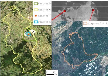
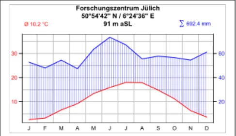
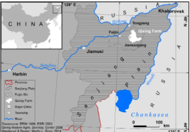
1.1 Concept of increasing spatial and temporal resolution 6 2.1 Schematics of active and passive satellite remote sensing 9 2.2 Overview of the study sites. . . 25 2.3 Walter Lieth climate diagram for Fujin, China. . . 26 2.4 Walter-Lieth Climate diagram for Jülich, Germany. . . 28 3.1 Location of the study site. . . 34 3.2 Workflow to optimize the Maximum Likelihood clas-
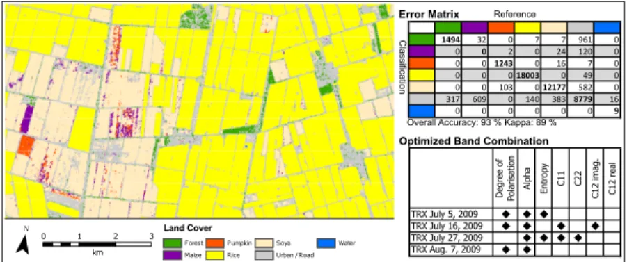
sification and find the input features resulting in the highest classification accuracy. . . 41 3.3 Comparison of the classifications of the smaller extent. 43 3.4 Optimized Maximum Likelihood Classification from all
radar data covering the smaller subset. . . 43 3.5 Optimized Maximum Likelihood Classification from all
data covering the smaller subset. . . 45 3.6 Best combination of one single radar acquisition with
the optical FORMOSAT2 image over the smaller area. 45 3.7 Accuracy comparison of the classifications from acqui-
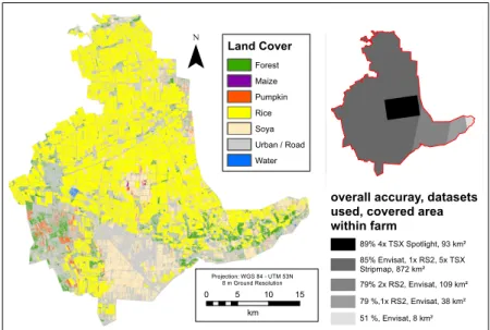
sitions with a wider coverage. . . 46 3.8 Combination of the best classifications from all mi-
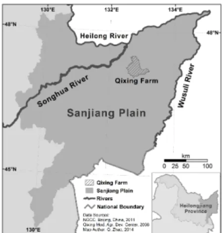
crowave images involved in this study to classify the whole area of the farm with the best possible accuracy. 47 4.1 Location of the study area Qixing Farm in Northeast
China. . . 65 4.2 Georeferencing workflow of the multi-source geospatial
data. . . 68
4.3 Field boundary data, before and after the georeferencing 72 4.4 Example of georeferenced multi-source remote sensing
images in comparison to the TerraSAR-X image. . . . 74 4.5 Georeferenced multi-source data for the study area of
Qixing Farm. . . 77 5.1 Location of the study site. . . 90 5.2 Workflow diagram to create the final LULC map from
TerraSAR-X images, the ground survey, and the exter- nal geodata. . . 94 5.3 Mean OA of the single dates and the multitemporal
approaches. . . 97 5.4 F1-scores of the classes in the single-date classifications
and the multitemporal accuracy. . . 98 5.5 Map of the final classification. . . 99 5.6 Mean error matrices of the two multitemporal methods.100 6.1 Location of the study region Rur Catchment and LULC
analysis of 2017. . . 120 6.2 Final Classification with a two times post classification
majority filter of the whole AOI covering about 2500 km
2129 7.1 Overview of the four acquired WorldView-2 Scenes . . 149 7.2 Overview of the area of interest on the four satellite
scenes. . . 149 7.3 Southwest looking photo of the maize field. . . 149 7.4 Northeast looking photo of the maize field. . . 149 7.5 Accuracy checkpoint 5 and its position in the 4 satellite
scenes. . . 153 7.6 Correlation of NDVI from WV-2 and CSM-derived
plant height, beginning of July . . . 155 7.7 Correlation of NDVI from WV-2 and CSM-derived
plant height, beginning of August . . . 155 7.8 Regression of the CSM-derived plant height from July
3rd and dry biomass. . . 156
List of Figures 7.9 Regression of the NDVI from WorldView-2 acquisition
from the 6th July and the dry biomass taken on 3rd July.156 7.10 Regression of the linear combination of CSM-derived
plant height and NDVI from WorldView-2 with the dry biomass. . . 156 7.11 Final dry biomass Map for the 2nd date, calculated
from WorldView-2 NDVI and CSM derived plant height using formula 7.1. . . 156 8.1 Cherry Picker with Riegl Scanner next to the maize field.168 8.2 Interferogram generated from the TDM pair of July
15, 2014 . . . 169 8.3 Multilooked Interferogram generated from the TDM
pair of July 15, 2014 . . . 170 8.4 Unwrapped Phase generated from the TDM pair of
July 15, 2014. . . 171 8.5 Geocoded DTM, generated from the TDM pair from
15.07.2014 (HH-Polarization images only) . . . 172 8.6 Heigth difference between June 1st and July 15th,
derived from TDM. . . 173 8.7 Heigth difference between June 1 st and July 26th,
derived from TDM. . . 174 8.8 Mean height values from HH- and VV-Polarisations
over of the maize fields of the region . . . 175 8.9 All pixel-wise extracted plant heights of the maize field
at two different dates. . . 176 9.1 Comparison of the resolutions of the remote sensing
input data of chapters 3, 5, and 6. . . 184
List of Tables
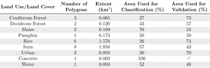
1.1 Overview of the different sensors and datasets that were combined, evaluated or analyzed in the different chapters . . . . 7 3.1 Field data collected during the 2009 growing season
that is covered by all remote sensing images. . . 35 3.2 Remote Sensing acquisitions that were used in this study. 35 3.3 Importance of input features for the smaller subset,
following the Maximum Likelihood optimization. . . . 48 4.1 Characteristics of the remote sensing images used for
chapter 4 . . . 67 4.2 Accuracy of the selected GCPs. . . 73 4.3 Accuracy of the independent check points. . . 75 5.1 Radar remote-sensing image statistics. . . 91 5.2 Overview of collected reference data. . . 92 5.3 Acquisition windows (AW) for optimal crop separation
in the Rur area. . . 93 5.4 Comparison of the two multitemporal approaches. . . 102 6.1 Metadata of the Sentinel-1, A and B, acquisitions used
in this study . . . 123 6.2 Sentinel-1a and Sentinel-1b acquisitions of the study
period. . . 124 6.3 Collected field data of crop distribution during the
growing season 2017 . . . 125
6.4 Error Matrix of the open data MDA classification shown in Figure 6.2. . . 130 6.5 Error Matrix of the MDA LULC classification with
optical data . . . 131 6.6 Comparison of the Producer’s Accuracy and User’s
Accuracy of crop classes of the study carried out by Bargiel (2017) and of the present study. . . 134 7.1 Absolute positional error of the WorldView-2 images. . 153 8.1 TanDEM-X Constellation (TDM) acquisitions that
were used in this study. . . 167
Abbreviations
AOI Area of Interest . . . 10 ALKIS German Authoritative Real Estate Cadastre
Information System . . . 125 ATKIS German Authoritative Topographic-Cartographic
Information System . . . 21 AW Acquisition Window . . . 87 CSM Crop Surface Model . . . 146 DEM Digital Elevation Model . . . 12 DLM Digital Landscape Model . . . 91 DLR German Aerospace Center. . . .167 DTM Digital Terrain Model . . . 164 EU European Union. . . .19 ESA European Space Agency . . . 36 FOSS Free and Open-Source Software . . . 118 GCP Ground Control Point . . . 60 GIS Geographic Information System . . . 12 GPS Global Positioning System . . . 152 GRD Ground Range Detected. . . .123 HRWS High Resolution Wide Swath . . . 18 ICASD International Center for Agro-Informatics and
Sustainable Development . . . 24
LULC Land Use / Land Cover . . . 1
LULCC Land Use / Land Cover Change . . . 1
LPIS Land Parcel Identification System . . . 21
MDA Multi-Data Approach . . . 19
NEST Next ESA SAR Toolbox. . . .36
NRW North Rhine-Westphalia . . . 27
NDVI Normalized Difference Vegetation Index . . . 146
NNI Nitrogen Nutrition Index . . . 147
OA Overall Accuracy . . . 33
PB Physical Blocks . . . 86
RF Random Forest. . . .18
SAR Synthetic Aperture Radar . . . 4
SNAP Sentinel Application Toolbox . . . 118
SI Sustainable Intensification . . . 1
SRTM Shuttle Radar Topography Mission . . . 13
TDM TanDEM-X Constellation . . . 8
TLS Terrestrial Laser Scanning . . . 8
TR32 Transregional Collaborative Research Centre 32 24
USGS United States Geological Survey . . . 10
1 Introduction
After almost a decade of declining world hunger, the number of undernourished people has been on the rise since 2014, reaching an estimated 821 million in 2017 (FAO et al. 2017). Additionally, more and wealthier people on planet earth are demanding more food and a more resource-intensive diet such as dairy products and meat (Godfray et al. 2018). This chapter provides an introduction into the challenges associated with agricultural production, Land Use / Land Cover Change (LULCC), discusses the need for Sustainable Intensification (SI) in agriculture, and identifies the role of remote sensing for LULCC, precision agriculture, and agricultural monitoring systems. Based on the data needs of those sectors, the overall objective of the study and the research questions are presented. Furthermore, an outline guides through the thesis.
1.1 Preface
There is immense pressure on global agricultural production to provide
sufficient food (Tilman et al. 2002). Agriculture already is and will
be threatened further by the implications of climate change (Wiebe
et al. 2015) and the scarcity of land (Lambin & Meyfroidt 2011),
the latter indicating the strong link of agricultural production to
Land Use / Land Cover (LULC) and LULCC. Global agriculture is
responsible for significant environmental issues as it directly accounts
for 14 % of global greenhouse gas emissions (IPCC 2014: 88), 70 % of
global freshwater usage (Rost et al. 2008), soil degradation (Parr
et al. 1992), and altering the global nitrogen cycle with many global
negative impacts (Vitousek et al. 1997). The latter being connected
to the release of heavy metals into the environment, pesticides, and fungicide abuse.
Not included in the statistics mentioned above is an indirect conse- quence that more land has been attributed to agricultural production over the last decades (Alexander et al. 2015). This increase is alarming as the global LULCC is the second highest contributor to the rising CO
2-concentration levels in the atmosphere, after the com- bustion of fossil fuels. Furthermore, current LULCC intensifies the conflict over land (Lambin & Meyfroidt 2011), leaving less space for nature (Tilman et al. 2002).
Rockström et al. (2017) claim for a SI in agriculture (Garnett et al. 2013), which aims to achieve future food security and solve the environmental issues of agriculture. SI is a complex challenge that can only be solved by a multitude of objectives and actions (McCarthy et al. 2018). One favorable principle is land sparing, which means increasing production through higher yields on already farmed land.
The alternative way of increasing production by using new land for farming would worsen the environmental impacts (Phalan et al.
2011).
Solving such social and environmental problems is strongly con- nected to land change science, which tackles environmental and soci- etal problems by understanding the dynamics of LULC as a coupled human-environment system (Turner et al. 2007). The initial crucial step to performing any land change science is observation and monitor- ing (Turner et al. 2007). However, global LULC- and LULCC-maps of adequate resolution in high quality are not available (Prestele et al. 2016), yet urgently needed, especially in the context of global food production (See et al. 2015).
Precision agriculture suits the described aims of SI, being described as an information technology used to improve production management and minimize environmental impacts (Whelan & Taylor 2013: 1).
This technology helps to fulfill SI by higher yields per area and also improves the environmental quality (Gebbers & Adamchuk 2010).
Most commonly, and especially when considering cropping systems,
the term precision agriculture is used synonymously for site-specific
1.1 Preface crop management (Whelan & Taylor 2013: 2). That term, however, refers more specifically to adopting the agronomic practices to the specific resource needs depending on the location. Those needs vary considerably not only from one field to another but also within fields.
Hence, through knowledge about the growing conditions at each location within the field, farming machines can apply site-specific management, such as fertilizer applications (Carr et al. 1991) or plant protection actions (Mahlein et al. 2012).
In addition to precision agriculture techniques, agricultural monitor- ing systems provide information about food production (Fritz et al.
2018). Such systems allow forecasting of commodity prices enabling preparation for food-market variations. Risks in the food supply chain can thereby be identified, resulting in greater food security (Wu et al.
2014).
Land change science, precision farming and agricultural monitoring Systems depend on the quality and availability of the input data to provide reliable results (Jones et al. 2017). Furthermore, Jones et al.
(2017) conclude that the limitations of current systems are due to a lack of available and usable data. The most prominent tool to acquire the needed data is remote sensing (Zhang et al. 2002; Pinter Jr et al.
2003). It can provide information about the environment, LULC, crop type, and the status of crops (Vinciková et al. 2010), which could not be generated with other methods because traditional methods, such as field surveys, are too time-consuming and expensive (Xie et al.
2008). Summaries of applications of remote sensing can be found in McNairn & Shang (2016) for crop tpe mapping, in Atzberger (2013) for agricultural monitoring systems, and in Mulla (2013) for
precision farming.
The ongoing development of optical and especially of radar remote sensing systems have created new potentials for dealing with the future challenges described above. The development of new sensors mainly provides increased resolution over larger areas. Advanced information processing is, however, needed to fully exploit the potential of such systems (Benediktsson et al. 2012).
One such actively researched remote sensing sensor category consists
of radar or microwave remote sensors. They have the advantage of providing images even at night, and can penetrate through clouds (Curlander & McDonough 1991a). Surprisingly, Whelan &
Taylor (2013) and Atzberger (2013) omit Synthetic Aperture Radar (SAR) remote sensing for precision farming and agricultural monitoring, respectively. Furthermore, as shown by Fritz et al.
(2018), only three out the eight most important global agricultural monitoring systems use active radar data. The reasons for that lack of tapping the full potential of SAR could lie in the complexity of the radar signal, limited radar sensor capabilities (Schmullius et al.
2015), and limited knowledge of how microwaves interact with surfaces (Woodhouse 2015: 28).
1.2 Overall Objective and Research Questions
This study is based on the need for high-quality, frequently updated LULC maps, including information about crop type, and on a gen- eral lack of available and usable geoinformation about agricultural production. Furthermore, it is framed by the opportunities of sensor developments, especially in the domain of microwave remote sensing, where case studies are urgently needed to demonstrate and evaluate the potential of the technology. Hence, this research’s objective is to obtain knowledge on how the combination of radar remote sensing, optical remote sensing, and other geodata can provide such necessary geoinformation for land use studies, precision farming, and agricultural monitoring systems.
This overall objective is subdivided into the following smaller ob-
jectives, which are sorted according to the principle of increasing
temporal and spatial resolution. Furthermore, the second and third
objectives presuppose the objectives one and two, respectively. All
objectives are under the assumption of using satellite remote sensing
data.
1.2 Overall Objective and Research Questions
1. Determining of LULC in agricultural landscapes.
2. Mapping crop types, especially the annually changing cultivated crops.
3. Detecting the in-field variability of crop traits such as plant vitality, height, and biomass.
For all of the objectives, the research interest is to acquire the geoinformation itself, but the fundamental research goal is to find, and if necessary to develop, the most opportune method to achieve the desired output. Based on these objectives described above, the following research questions are derived:
• Which methods are best suited to achieving the objectives 1–3 from different remote-sensing image products in appropriate quality?
• How can existing external geodata be incorporated in the pro- cess? What is its benefit?
• Can the results be improved by incorporating existing geographic data, such as existing cadastral data about the agricultural land?
• How can radar remote sensing be used alone and in combination with optical remote sensing and external geodata to obtain LULC, crop type and crop traits?
• What are the most crucial remote sensing data characteristics for those objectives and what is their effect on the quality of the output?
• What are the essential characteristics of radar remote sensing images for those objectives?
• Which data characteristics are useful for evaluating the results?
• How can the desired outputs be generated cost-effectively and
efficiently?
1.3 Outline
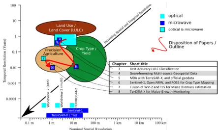
After the Introduction (1), the chapter Basics (2) focuses on the main concept of remote sensing for introducing the different kinds of data and their characteristics. A short introduction to the study sites is given next. Following that, the research papers are given in the chapters 3 to 8. They are organized based on the concept of increasing temporal and spatial resolution for selected applications from coarse to high, as shown in Figure 1.1. Table 1.1 demonstrates the different sensors and other datasets used in the chapters, including the research objective that is primarily pursued.
WorldView-
FORMOSAT-2
Crop Type / Yield Precision
Agriculture Land Use / Land Cover (LULC)
TerraSAR-X / Tnd Sentinel-1
Worldview-2 (multi)
WorldView-2 (pan)
optical microwave optical & microwave 4 3
5
6 7
8
Disposition of Papers / Outline
Figure 1.1: Concept of increasing spatial and temporal resolution, modified according to the relevant applications of this study. Modified after Jensen (2007).
The first research study, presented in chapter 3, introduces an
innovative method to obtain general LULC, including crop type, from
1.3 Outline
Satellite Images Diverse Geodata
X-band
SAR C-band
SAR Optical Elevation
Models In Situ
Data
Chapter
Short title Study site TerraSAR-X TanDEM-X EnvisatASAR Radarsat-2 Sentinel-1 FORMOSAT-2 WorldView-2 S.R.T.M. DGM-1 OfficialGeodata CropDistribution TLS Biomass ResearchObjective
3 Best Accuracy
LULC Classification Qixing
China ı ı ı ı ı ı 1+2
4 Georeferencing Multi-source
Geospatial Data Qixing
China ı ı ı ı 2
5 MDA with TerraSAR-X
and official geodata Subset of
the TR32 ı ı ı ı 1+2
6 Sentinel-1, Open.NRW, and FOSS for Crop Type Mapping Whole
TR32 area ı ı ı ı 1+2
7 Fusion of WV-2 and TLS for Maize Biomass Estimation Selhausen
TR32 ı ı ı ı 3
8 TanDEM-X for Maize
Growth Monitoring Selhausen
TR32 ı ı ı ı 3
Table 1.1: Overview of the different sensors and datasets that were combined, evaluated or analyzed in the different chapters
SAR and optical data in the study site Qixing farm, Heilongjiang, China. Chapter 4 introduces the novel idea of using the high geometric accuracy of the SAR satellite TerraSAR-X to produce a high-resolution geometric reference image for the diverse geospatial data of different scales and resolutions, thus making it possible to include any externally available data into the classification process, especially such data with a non-ideal geometric accuracy. Chapter 5 demonstrates the fusion of SAR remote sensing with such external data. The result is an enriched LULC map, containing the annual crop distribution obtained from the SAR data, as well as the LULC classes from the external data.
In chapter 6, this idea is extended by relying on open data and open
software only, making the approach much more low-cost. Once the
annual crop distribution is available, additional analysis of the field
crop status can be performed. Innovative examples of crop status
monitoring are demonstrated in chapters 7 and 8. As can be seen
in Figure 1.1, the resolution needs are greatly increased for such
applications. Chapter 7 is based on high-resolution optical images
from WorldView-2, which have a spatial resolution and accuracy high
enough to allow monitoring of within-field crop variances. Chapter
8 introduces the new innovative method of how to determine the
plant height parameter from multitemporal satellite acquisitions from
the TanDEM-X Constellation (TDM). The images had to be gained
in the experimental, high-resolution, spotlight mode. Validation is
performed using highly precise field measurement from Terrestrial
Laser Scanning (TLS). In chapter 9, an overall discussion across the
chapters and a discussion about putting the conclusions gained from
the research in a scientific context are pursued. A conclusion is given
in chapter 10.
2 Basics
2.1 Remote Sensing
Remote sensing is defined as "the art and the science of obtaining information about an object without being in direct physical contact with an object" (Jensen 2007: Preface). Typically the sensors are mounted onto aircrafts, satellites (Emery & Camps 2017) and nowa- days also drones (Bendig et al. 2012). Also, ground-based sensors are possible, sometimes called proximal remote sensing. The present work focuses mainly on sensors mounted on board satellites flying in low earth orbit (LEO). Depending on the underlying principle, the sensors used can be divided into passive, optical, and active, mostly microwave, sensors (compare Figure 2.1. The concept of resolution – spatial, temporal, and spectral – guides the reader deeper into the
topic of satellite-based remote sensing.
(A) (B)
Figure 2.1: Schematics of passive (A) and active (B) satellite re-
mote sensing, own representation, inspired by Albertz
(2009: 10)
2.1.1 Optical Remote Sensing
The basic measurement principle of optical remote sensing is the de- tection of sunlight reflected from the earth’s surface to create images (Emery & Camps 2017: 85). Depending on the sensor type, the intensity of electromagnetic waves in the visible and infrared part of the spectrum is measured. As depicted in Figure 2.1 (A), the radiation travels through the atmosphere before interacting with the earth’s surface and again on the way towards the sensor. Conse- quently, such systems rely on an undisturbed path of the radiation through the atmosphere, which can be blocked by clouds (Emery
& Camps 2017: 86). Additionally, the radiation interacts with the atmosphere while traveling through it. Atmospheric corrections are hence mandatory when accounting for such atmospheric effects in the imagery (Liang 2005: 197).
Under a clear sky, optical systems can retrieve spectral signals from the earth’s surface. This spectral signature depends mainly on the chemical properties of an imaged land surface, and many characteristics can be retrieved.
The numerous deployed optical satellite systems differ quite consid- erable concerning their different scanning principles (Heipke 2017: 12- 13). They either scan a long strip along their travel path or are tasked to acquired images over a specific Areas of Interest (AOIs).
Among the ones that provide a long strip, the Landsat system, oper-
ated by the United States Geological Survey (USGS), is by far the
most prominent. It provides the longest temporal record of satellite
images. Most locations on earth were successfully imaged at least
annually for the last 40 years (Roy et al. 2014). Although the current
Landsat-8 system is technically superior to the first Landsat-1, its
flight path is still the same, allowing time series analysis over the last
four decades. Other satellite systems being tasked to take images
are often company-owned, and monitoring of an AOI is usually done
per request, which can be expensive. Such systems can be usually be
turned towards the AOI once it is in sight. They generally allow a
higher resolution (temporal, spectral and spatial) (Benediktsson
2.1 Remote Sensing et al. 2012). A complete introduction into optical remote sensing is given by Heipke (2017), Campbell & Wynne (2011), Albertz (2009), Jensen (2007), and Lillesand et al. (2004).
2.1.2 Microwave Remote Sensing
The fundamental basis of microwave or radar remote sensing is the send and receive principle. An impulse of electromagnetic radiation is sent and received. The time delay between sending and receiving the signal is measured along with the intensity of the returned signal.
The measured intensity of the signal depends on a complex electro- magnetic interaction between the radar waves and the scene, and scattering depends on morphological and dielectric properties of the investigated medium (Emery & Camps 2017: 298). By combining multiple measurements of the intensity of the backscattered signal, it is possible to create a radar image of the observed surface. The modern, most widespread imaging radar technique is the Synthetic Aperture Radar (SAR) (Ulaby & Long 2014: 3).
Radar wavelengths used for remote sensing are divided into bands (Jutzi et al. 2017: 87). The shortest wavelength used by satellites is the X-band with a wavelength of about 3 cm. It is characterized by a small to no penetration depth into the examined medium; this is then characterized as surface remote sensing. The waves of the C-band are approximately 5 cm large and show a higher penetration depth. Penetration is further maximized with longer waves such as the ones from L-band (7.5 – 15 cm). Under the conditions of complete penetration into the medium, the process is described as volume scattering. The waves shorter than the X-band and longer than the L- band do not play a significant role for satellite remote sensing because they are significantly influenced by the atmosphere. However, the most important rule of thumb when choosing the wavelength for an application is that the dimensions of the structures under investigation should be roughly the same size as the wavelength (Emery & Camps 2017: 299).
Using polarimetric methods, the primary scattering processes within
a resolution cell can be determined (Lee & Pottier 2009). A first distinction can be made between surface and volume scattering. In the case of surface scattering, it can also be determined whether the number of scattering processes is odd or even. Double, i.e., an even number of reflections, is typical for urban areas. Typical for urban environments is also the occurrence of singular strong backscatterers, which manifest themselves as bright points in the radar image. The backscatter from rural areas is usually characterized by several so-called distributed scatterers per dissolution cell. Such distributed scatterers within one resolution cell are the cause of one major drawback of microwave images: – the grainy "salt and pepper"- like noise in all SAR images, which is called speckle. It makes visual interpretation more difficult and adds additional difficulty for image processing. Different techniques exist to deal with speckle:
• Multilooking: Neighbouring pixels are treated as individual radar measurements, and a new image that has a lower spatial resolution but contains less speckle is computed.
• Temporal Averaging: Images from SAR time-series are partic- ularly well suited to temporal averaging. In a time series, all images are made from almost the same satellite position. That means that the geometric distortions induced by relief are the same in all images.
• Speckle Filters: Mostly focal filters with moving windows are developed to preprocess the SAR images specifically for different applications. In general, they seek to obtain the image character- istics with bright scatterers and spatially average homogeneous areas.
A central processing of the images captured by radar sensors is the
conversion into a map projection. It is a prerequisite of further analysis,
e.g., using a Geographic Information System (GIS). A common
methodology for the projection is the range-doppler terrain correction
and involves using a Digital Elevation Model (DEM) (Curlander
2.1 Remote Sensing
& McDonough 1991a). During this process, the height error of the DEM translates into a horizontal error of the processed radar image.
Inaccurate elevation data can therefore be a source of error for the correct georeferencing of radar data. In addition to this correctable error, SAR images also exhibit relief-induced distortions due to their sideways viewing direction. While foreshortening is mainly corrected during the projection process, areas with radar shadow and layover contain no usable information (Richards 2009: 111).
Interestingly, elevation data is not only used to process SAR data but can also be generated by SAR sensors. The acquisition of SAR images from several acquisition positions allows interferometric analy- ses (Richards 2009: 183). Single pass and repeat-pass interferometry are the two alternative here. Single-pass interferometry is particularly well-suited to large-area topographic mapping. Famous examples are the global elevation models created by the Shuttle Radar Topography Mission (SRTM) (Rodriguez et al. 2006) and the TDM (Krieger et al. 2007). Repeat-pass interferometry is mainly used for detecting changes of the surface elevation between the acquisitions, such as in the mapping of earthquakes (Massonnet et al. 1993).
An extension to interferometry is tomography, in which SAR images from several positions are combined to obtain the vertical structure of the features in a scene. SAR sensor development is actively researched with awaited improvement from multifrequency SAR (Rosen et al.
2015), digital beamforming (Younis et al. 2003), multistatic sensor constellations (Kraus et al. 2017), and improved orbit constellations (Moreira et al. 2013) such as High Orbit SAR.
For a more complete description of radar remote sensing, its varied applications, and the historical development of the discipline, the interested reader is referred to the excellent textbooks by Woodhouse (2015), Ulaby & Long (2014), and Richards (2009).
2.1.3 Spectral Resolution
The spectral resolution is the number of different bands captured by
remote sensing systems. In optical imaging systems, a distinction is
made between multispectral and hyperspectral systems, depending on the number of used bands. Multispectral systems sense the amount of energy in approximately 3–15 bands in particularly suitable areas of the optical, infrared, and thermal range. Hyperspectral systems scan the spectrum in specific areas with a continuous sequence of bands. Depending on sensor performance, several hundred bands can be scanned simultaneously.
With radar sensors, the concept of spectral resolution has to be widened. Due to technical limitations on satellites, only systems with one wavelength are currently in use (Ulaby & Long 2014). However, additional information about the examined surface is acquired by measuring the single frequency radar signal in different polarizations (Cloude 2010). Four different polarization combinations can be ob- tained by sending and measuring the radar signal horizontally and vertically. Polarimetric decompositions, such as the Pauli analysis, allow determination of the dominant scattering process on the ground.
Odd (mostly single), even (mostly double) bounces and volume scat- tering can be distinguished. The polarimetric capabilities of SAR sensors increase the information content of the measurement, as dif- ferent bands do in the optical domain. Hence, in the context of this work, not only the different radar wavelengths but also the amount of measured polarizations are considered when assessing the spectral resolution of the SAR images.
2.1.4 Spatial Resolution
The spatial resolution is the ability of a sensor system to separate signals from two adjacent objects (Emery & Camps 2017: 295). In most remote sensing scenarios, the size of a pixel of the analyzed images is understood as the spatial resolution. For most analyses based on optical data, this principle is sufficient. The optical sensors are often designed in such a way that one resolution cell of the sensor (Instantaneous Field of View) covers one pixel in the produced image.
The size of a pixel, in reality, is then given as the spatial resolution of
the sensor. To a certain extent, it depends on the viewing angle, with a
2.1 Remote Sensing better resolution below the center of the sensors. However, the spatial resolution is mainly determined by the sensor design. Typical spatial resolution of space-borne imaging systems are MODIS (250–500 m) (Chen, Fedosejevs, et al. 2006), Landsat (15–30 m) (Roy et al.
2014), Sentinel-2 (10–60 m) (Drusch et al. 2012), or WorldView-2 (0.5–2 m) (Updike & Comp 2010).
For SAR sensors, it is important to keep the original definition of spatial resolution as the ability to separate two objects. The side- looking geometry of SAR imaging makes determining the resolution more complex. First, a distinction must be made between azimuth (along-track) and range (cross-track) resolution. The range resolution depends on the available bandwidth of the system and the incidence angle (◊). Contrary to optical systems, the range resolution is better, the steeper the angle. In consequence, SAR images have an increasing resolution the further away the sensor is (Woodhouse 2015: 269).
Even more surprising is the determination of the azimuthal resolution of SAR images: The maximum possible resolution is equal to half of the length of the antenna (Woodhouse 2015: 274). Neither the wavelength nor the distance of the sensor from the target plays a role here (Emery & Camps 2017: 295).
SAR sensors offer the possibility to operate in different modes.
During Spotlight operation, the antenna is steered during the overflight in such a way that the target is sensed for a longer time. This has the advantage of an increased azimuthal resolution, but the disadvantage of a reduced swath width (Woodhouse 2015: 287). To cover vast areas, the spatial resolution can also be reduced for the benefit of a very wide swath using the ScanSAR mode. This mode is suited for regional to global scale monitoring as it provides the necessary coverage (Woodhouse 2015: 287).
2.1.5 Temporal Resolution
Temporal resolution is the time it takes a sensor system to monitor
the same area again. It is an essential consideration in all remote
sensing applications (Campbell & Wynne 2011: 286). The temporal
resolution required depends on the specific application (Jensen 2014).
Apparently, in the case of a disaster such as a flood, it is most important to gain information about the AOI as quickly as possible while, for planning purposes, an acquisition dating a couple of months back might be sufficient.
For satellite remote sensors, the available temporal resolution de- pends on the orbit and the scanning pattern of the satellite (Njoku 2013: 146). Continuous optical monitoring systems usually have a lim- ited temporal resolution as it depends on the revisit time, which is the time until the satellite reaches the same position in orbit. Landsat-8, for example, has a revisit time of 16 days (Roy et al. 2014). Only in these precisely scheduled time windows is it possible for these sensors to take images. If clouds obscure a clear view on the earth’s surface during these time windows, no information can be gained from the surfaces. The optical systems with steering capabilities potentially have a much higher temporal resolution. WorldView-2
1, for example, is equipped with extreme steering capabilities, giving the satellite an almost daily chance to acquire an image (Updike & Comp 2010).
However, to get an analyzable image, the AOI has to be cloud-free, and the image is only taken per request. As each acquisition has a high price, a high temporal resolution is expensive. Furthermore, the steerable satellite scan the earth’s surface at varying off-nadir angles.
Analyzing these images needs consideration of the bidirectional re- flectance distribution function (Leroy & Roujean 1994), resulting in increased analysis complexity.
In the case of clouds, SAR imaging is the only alternative, as the microwaves can penetrate clouds (Ulaby & Long 2014; Woodhouse 2015). There is less difference between the potential and the actual imaging capabilities of SAR sensors, giving them an increased tempo- ral resolution. The recently deployed Sentinel-1 constellation (Torres et al. 2012), for example, has a continuous monitoring principle with a revisit time, from the same satellite orbit, of 6 days. As the swaths of
1Images of the WorldView-2 Satellite system are used in the study described in chapter 7