Accepted Article
Solar Signals in CMIP-5 Simulations: The Ozone Response
L. L. Hood,
a∗S. Misios,
bD. M. Mitchell,
cE. Rozanov,
d,eL. J. Gray,
c,fK. Tourpali,
bK. Matthes,
g,hH. Schmidt,
iG. Chiodo,
j,kR. Thi´eblemont,
gD. Shindell,
lA. Krivolutsky,
maLunar and Planetary Laboratory, University of Arizona, Tucson, Arizona, USA.
bLaboratory of Atmospheric Physics, Aristotle University of Thessaloniki, Thessaloniki, Greece.
cAtmospheric, Oceanic and Planetary Physics, University of Oxford, Oxford, UK.
dPhysikalisch-Meteorologisches Observatorium, World Radiation Center, Davos Dorf, Switzerland.
eInstitute for Atmospheric and Climate Science, ETH, Zurich, Switzerland.
fNERC, National Centre for Atmospheric Science (NCAS), UK.
gGEOMAR Helmholtz Centre for Ocean Research Kiel, Kiel, Germany.
hChristian-Albrechts Universit¨at zu Kiel, Kiel, Germany.
iMax Planck Institute for Meteorology, Hamburg, Germany.
jDepartamento Fisica de la Tierra II, Universidad Complutense de Madrid, Madrid, Spain.
kApplied Physics and Applied Mathematics, Columbia University, New York, New York, USA.
lNicholas School of the Environment, Duke University, Durham, North Carolina, USA.
mLaboratory for Atmospheric Chemistry and Dynamics, Central Aerological Observatory, Moscow, Russia.
∗Correspondence to: LPL, Univ. of Arizona, 1629 E. University Blvd., Tucson, Arizona 85721 USA. E-mail:lon@lpl.arizona.edu
A multiple linear regression statistical method is applied to model data taken from the Coupled Model Intercomparison Project, phase 5 (CMIP-5) to estimate the 11-yr solar cycle responses of stratospheric ozone, temperature, and zonal wind during the 1979-2005 period. The analysis is limited to the six CMIP-5 models that resolve the stratosphere (high-top models) and that include interactive ozone chemistry. All simulations assumed a conservative 11-yr solar spectral irradiance (SSI) variation based on the NRL model. These model responses are then compared to corresponding observational estimates derived from two independent satellite ozone profile data sets and from ERA Interim Reanalysis meteorological data. The models exhibit a range of 11-yr responses with three models (CESM1-WACCM, MIROC-ESM-CHEM, and MRI-ESM1) yielding substantial solar-induced ozone changes in the upper stratosphere that compare favorably with available observations. The remaining three models do not, apparently because of differences in the details of their radiation and photolysis rate codes.
During winter in both hemispheres, the three models with stronger upper stratospheric ozone responses produce relatively strong latitudinal gradients of ozone and temperature in the upper stratosphere that are associated with accelerations of the polar night jet under solar maximum conditions. This behavior is similar to that found in the satellite ozone and ERA Interim data except that the latitudinal gradients tend to occur at somewhat higher latitudes in the models. The sharp ozone gradients are dynamical in origin and assist in radiatively enhancing the temperature gradients, leading to a stronger zonal wind response. These results suggest that simulation of a realistic solar-induced variation of upper stratospheric ozone, temperature and zonal wind in winter is possible for at least some coupled climate models even if a conservative SSI variation is adopted.
Key Words: SolarMIP, solar, stratosphere, ozone, CMIP-5, natural variability
c 2013 Royal Meteorological Society Prepared usingqjrms4.cls
This article has been accepted for publication and undergone full peer review but has not been through the copyediting, typesetting, pagination and proofreading process, which may lead to differences between this version and the Version of Record. Please cite this article as doi:
10.1002/qj.2553
Accepted Article
1. Introduction
As reviewed by Mitchell et al. (2014a) (hereafter referred to as Paper 1), the stratosphere containing the ozone layer represents a key link through which solar variability can produce perturbations of tropospheric circulation. Solar influences on surface climate
5
can, in principle, be due either to solar irradiance variations or changes in corpuscular radiation (energetic charged particles), or both (see, e.g., section 4 of the review by Gray et al. 2010).
Influences of solar irradiance variability can be further divided into a so-called “bottom-up” category, involving direct penetration
10
of solar radiation at wavelengths greater than about 300 nm to the lower troposphere, and a “top-down” category, involving effects of solar ultraviolet (UV) radiation on the upper atmosphere with indirect dynamical effects at lower levels. Because of the important role of ozone, which is mainly produced by solar UV
15
radiation, in radiatively heating the stratosphere and because solar UV variability is relatively large (up to ∼ 6% near 200 nm over an 11-yr cycle compared to∼0.1% at wavelengths >300 nm), top-down solar irradiance forcing is believed to be a non- negligible component of solar-induced climate variability (Haigh
20
1994; 2003; Kodera and Kuroda 2002; Matthes et al. 2006; Meehl et al. 2009; Hood et al. 2013; Gray et al. 2013).
There are a number of sources of uncertainty in designing a general circulation model (GCM) that is able to simulate the observed top-down component of solar irradiance-induced climate
25
change. These include uncertainties in solar spectral irradiance (SSI) variability itself, uncertainties in observational estimates for the solar-induced stratospheric and surface climate response, and uncertainties in the model formulation (see section 2.2 below).
The nature and magnitude of SSI variability has been a topic
30
of increased attention during the last decade. Due to a lack of direct, long-term measurements of SSI, proxy-based models have previously been developed by several groups using indirect measurements such as sunspot area, the solar 10.7 cm radio flux (F10.7), and the solar Mg II core-to-wing ratio (see the review
35
by Ermolli et al. 2013). These SSI models have been extensively employed in climate model simulations. For example, the SSI model developed at the U.S. Naval Research Laboratory (NRL SSI; Lean et al. 1995; Lean 2000; Wang et al. 2005) has been
adopted for use by most models in the most recent Coupled Model
40
Intercomparison Project (CMIP-5) (Taylor et al. 2012).
New direct satellite-based measurements of SSI began to be obtained in 2003 by the SORCE (SOlar Radiation and Climate Experiment) (e.g., Harder et al. 2009). As reviewed by Ermolli et al. (2013), the SORCE measurements differ in major ways from
45
the proxy-based models and some of these differences may be a consequence of instrument degradation with time (e.g., Lean and DeLand 2012). In particular, a large SSI decrease in the 200 to 320 nm range was measured by SORCE during the decline of solar cycle 23 that was four to six times larger than estimated by proxy-
50
based models. Ermolli et al. (2013) conclude that a lower limit on the magnitude of the SSI solar cycle variation is represented by the NRL SSI model while the SORCE measurements may represent an upper limit. However, results of recent efforts to account for and correct instrument degradation effects in the SORCE SSI data
55
(e.g., Woods 2012) suggest that the measured upper limit will be revised downward considerably.
This is the second in a series of analyses performed as part of the SPARC SOLARIS-HEPPA SolarMIP project (Solar Model Intercomparison Project). In Paper 1 (Mitchell et al. 2014a),
60
multiple linear regression (MLR) was applied to assess the 11- yr solar cycle component of both stratospheric and surface climate variability in the full suite of more than 30 models that contributed to the CMIP-5 comparison study. The analysis focused on the 13 models that resolve the stratosphere (high-top models) and
65
some evidence was obtained that these models are able to simulate better the surface response during northern winter than are low- top models. However, as a whole, most of the high-top models did not reproduce either the magnitude or latitudinal gradients of solar-induced temperature responses in the upper stratosphere
70
that are estimated using most meteorological reanalyses (see also Mitchell et al. 2014b). For this reason, the high-latitude dynamical responses that lead to significant top-down forcing of regional surface climate were also not well simulated in most of the high- top models.
75
In this paper, the model characteristics that yield a reasonable agreement of solar signals with available observations of the stratosphere are examined further. Specifically, multiple linear regression (MLR) is applied to compare in more detail solar
Accepted Article
signals in a subset of the 13 high-top CMIP-5 models considered
80
in Paper 1, i.e., the 6 models that included coupled interactive ozone chemistry (as opposed to those whose stratospheric ozone variability was prescribeda priori). Attention is focused especially on the model response of stratospheric ozone (which was not considered in Paper 1), as well as those of temperature and
85
zonal wind, and comparisons are made to selected observational estimates for the time period after 1979 when continuous global satellite remote sensing measurements began.
In many respects, this study builds on a previous work by Austin et al. (2008; see also Chapter 8 of SPARC-CCMVal
90
2010). The latter authors analyzed solar cycle signals of ozone and temperature in a series of simulations of coupled chemistry climate models (i.e., general circulation models with coupled interactive chemistry) over various periods during the last half of the 20th century. The employed models did not have coupled
95
oceans but were forced at their lower boundaries using observed sea surface temperatures (SSTs). It was shown that the model ozone results were generally in agreement with observations at tropical latitudes (e.g., Soukharev and Hood 2006), yielding a double-peaked vertical structure with a maximum response
100
near 3-4 hPa of two to three per cent over a solar cycle, a minimum near 20 hPa, and a secondary maximum in the lower stratosphere. The upper stratospheric response is primarily a consequence of increased photolytic ozone production while the lower stratospheric response is believed to have a transport origin,
105
resulting mainly from a slowing of the upwelling branch of the mean meridional (Brewer-Dobson) circulation near solar maxima (Kodera and Kuroda 2002; Hood and Soukharev 2012).
However, a long-standing issue is whether part or all of the tropical lower stratospheric 11-yr response derived from
110
observations during the satellite era may be a consequence of aliasing from the aerosol effects of two major volcanic eruptions, El Chich`on and Pinatubo, that fortuitously occurred following solar maxima in 1982 and 1991 (Solomon et al. 1996; Lee and Smith 2003; Chiodo et al. 2014). Austin et al. (2008) tested this
115
by comparing solar regression results with and without including an aerosol term in the MLR statistical model. They found little impact when analyzing model data over the 1960-2005 model period.
But some model chemistry schemes may be more sensitive
120
to volcanic aerosol injections than others. For example, Dhomse et al. (2011) analyzed transient simulations using the SLIMCAT chemical transport model developed at the University of Leeds (Chipperfield 1999; 2006) over 1979-2005 and found that the modeled ozone solar response in the tropical lower stratosphere
125
is amplified by aliasing from the volcanic eruptions. This was apparently because the model overestimates ozone losses during high aerosol loading periods. Further investigation of the volcanic aerosol aliasing issue in coupled climate models is therefore needed.
130
In section 2, the 6 high-top CMIP-5 models with interactive ozone chemistry are described and the MLR statistical method that is applied to the model data is summarized. Results of the analysis for annually averaged monthly solar regression coefficients for stratospheric ozone and temperature over the
135
1979-2005 period are presented and compared for the 6 models in section 2.5. Annual mean MLR analyses of model data are also carried out for time periods prior to 1979 when there were no major volcanic eruptions to assess further the sensitivity of the different model MLR results to volcanic aerosol aliasing during
140
the 1979-2005 period. In section 3, previous efforts to estimate observationally the 11-yr solar-induced responses of stratospheric ozone, temperature, and zonal wind using data acquired after the initiation of continuous global satellite measurements in 1979 are first briefly reviewed. Then, selected observations-based estimates
145
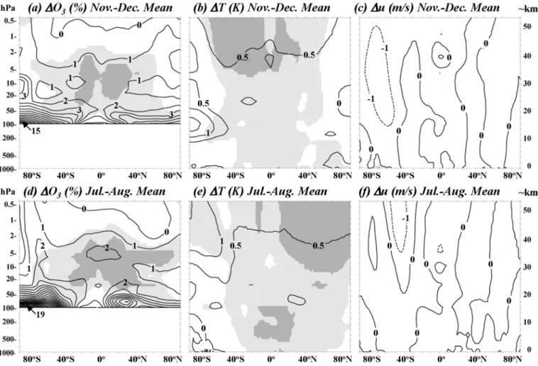
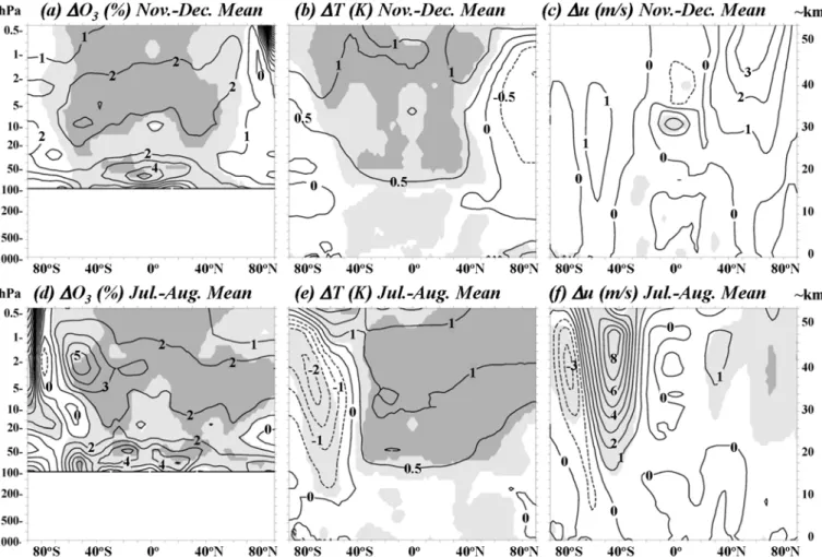
for these responses are presented for comparison with the model results. Next, the 11-yr solar signals in ozone, temperature, and zonal wind for the 6 models are examined in more detail for the northern early winter (Nov.-Dec.) and southern mid-winter (Jul.-Aug.) periods when observations indicate the strongest solar-
150
induced latitudinal gradients in ozone/temperature and the largest enhancements of the polar night jet in both hemispheres. A summary and further discussion are given in section 4.
2. Models, Statistical Method, and Annual Mean Results
2.1. Models
155
Table 1 lists the 6 high-top CMIP-5 models with interactive chemistry that are considered here. The institutes that were mainly
Accepted Article
responsible for producing these models are as follows: CESM1- WACCM - U.S. National Center for Atmospheric Research, Boulder, Colorado; MIROC-ESM-CHEM - University of Tokyo,
160
NIES, and JAMSTEC, Japan; MRI-ESM1 - Meteorological Research Institute of Japan, Tsukuba City, Japan; GFDL- CM3 - U.S. National Oceanic and Atmospheric Administration, Geophysical Fluid Dynamics Laboratory, Princeton, New Jersey;
GISS-E2-H and GISS-E2-R - U.S. National Aeronautics and
165
Space Administration, Goddard Institute for Space Studies, New York, New York. The two GISS models differ only in the nature of the coupled ocean model (Shindell et al. 2013). The GISS-E2- R model used the “Russell” ocean (Russell et al. 1995) while the GISS-E2-H model used the Hybrid Coordinate Ocean Model (Sun
170
and Bleck 2006). All models were required to produce at least one “historical” simulation over the 1850 to 2005 period with observed forcing consisting of solar spectral irradiance variations, volcanic sulfate aerosol, and greenhouse gas emissions (Taylor et al. 2012). Effects of energetic charged particle precipitation
175
were generally not included, except for WACCM, which has a parameterization for increased odd nitrogen production in the thermosphere as a function of the geomagnetic Kp index (Marsh et al. 2007). All of the models considered here adopted the NRL SSI model (Wang et al. 2005). Two of the models (CESM1-WACCM
180
and GFDL-CM3) also scaled the total solar irradiance (TSI) by a constant factor of 0.9965 to agree with SORCE Total Irradiance Monitor measurements (Kopp et al. 2005).
In the table, column 2 lists the number of ensemble members that were available for analysis for the period after 1979. Three
185
of the models (GFDL-CM3, GISS-E2-H, and GISS-E2-R) were applied to produce an ensemble of 5 historical simulations each.
The remaining three (CESM1-WACCM, MIROC-ESM-CHEM, and MRI-ESM1) performed one historical simulation each. In addition, CESM1-WACCM carried out three shorter simulations
190
for the 1955-2005 period with initial conditions taken from the single historical run (Marsh et al. 2013). Therefore, a total of 4 members are available for CESM1-WACCM for the period after 1979 when continuous global satellite observations became available. Columns 3 and 4 list the approximate vertical and
195
horizontal spatial resolutions of each model in the stratosphere (∼3 hPa). The vertical resolutions at this level are comparable
(∼ 2-3 km) for all models except for MIROC-ESM-CHEM, which has a resolution near 1 km. The horizontal resolutions are also comparable (several degrees of latitude or longitude at low
200
latitudes) except for MRI-ESM1, which has a higher resolution near 1 degree. Column 5 lists the approximate model tops in km.
These range from∼140 km for CESM1-WACCM to∼66 km for the two GISS models. Column 6 indicates whether each model simulates a QBO and whether the modeled QBO is internally
205
generated (spontaneous) or whether it is forced (nudged) to agree with observational constraints. Four of the models have no QBO while MIROC-ESM-CHEM has a spontaneous QBO and CESM1-WACCM has a nudged QBO. Finally, column 7 lists at least one recent reference for each model.
210
2.2. Model Radiation and Photolysis Rate Codes
According to published descriptions, all of the 6 coupled climate models considered here used up-to-date interactive chemistry schemes. The main characteristics of the chemistry schemes for 5 of the 6 models (CESM1-WACCM, MIROC-ESM-CHEM,
215
GFDL-CM3, GISS-E2-R, and GISS-E2-H) have been previously described in detail by Eyring et al. (2013; see their Appendix A). The chemistry scheme used in the MRI-ESM1 model, which provided data to the CMIP-5 archive at a later time, has been summarized by Yukimoto et al. (2011; see also Shibata et al. 2005
220
and Deushi and Shibata 2010). In addition, the model radiation codes, including methods for simulating heating from volcanic aerosols in the lower stratosphere, are described in detail in the references listed in Table 1.
However, the modeled response of stratospheric ozone and
225
temperature to 11-yr SSI forcing depends strongly on the detailed treatment of the solar UV irradiance in the 120-300 nm spectral range. Experiments using a 1-D radiative-convective-chemical model presented by Shapiro et al. (2013; see their Figure 2) are helpful for demonstrating that this is the case. In particular, they
230
showed using the NRL SSI data set that the increase in ozone mixing ratio in the stratosphere caused by an increase in solar UV radiation is mainly due to enhanced ozone production by O2
photolysis with a maximum near 40 km altitude. The increase in the 40-60 km layer is related to O2 absorption in the 121-200
235
nm interval (Schumann-Runge bands), while below 40 km the
Accepted Article
main spectral contribution is from the Herzberg continuum (200- 242 nm). A negative ozone response is expected in the middle mesosphere, driven by the increase of hydrogen radicals resulting from water vapor photolysis by SSI in the SRB and at the Lyman-
240
αline. Both the positive ozone response centered near 40 km and the negative response peaking in the middle mesosphere (∼68 km) have been confirmed observationally using satellite remote sensing measurements on the solar rotational (∼ 27-day) time scale (e.g., Hood 1986, Keating et al. 1987, Hood et al. 1991). The
245
absorption at the Lyman-αwavelength by O2is also responsible for a strong expected ozone increase in the upper mesosphere.
Ozone photolysis in the 240-300 nm spectral range leads to ozone loss partly compensating the influence of enhanced O2photolysis above 30 km.
250
The expected temperature response to an enhancement of solar UV radiation is always positive and has two maxima at the stratopause and mesopause (e.g., Shapiro et al. 2013). The mesopause maximum is defined mostly by oxygen absorption in the SRB and in the Lyman-αline. In the 50-70 km layer, the SRB
255
and Herzberg continuum contribution dominates, while below 50 km, ozone absorption in the Herzberg continuum and Hartley bands (200-300 nm) is the main contributor to the overall heating.
For regions where the influence of dynamics is not crucial (e.g., the tropical middle to upper stratosphere and lower mesosphere),
260
differences in modeled ozone and temperature responses to increases in SSI can potentially be explained by different representations of the photolysis and radiative heating responses.
Therefore, a detailed consideration of the individual model codes is necessary. It should be noted however that the magnitude of the
265
thermal response depends not only on the details of the shortwave radiation codes but also on the quality of the long-wave part of the codes because the net temperature change is a balance between solar heating and infrared cooling.
CESM1-WACCM
270
The model version participating in CMIP-5 is described by Marsh et al. (2013). For wavelengths>200 nm and at altitudes below 65 km, the heating rates are calculated using the scheme of Briegleb (1992), which is based on the two-stream delta- Eddington approximation (see also Briegleb and Light 2007). The
275
solar visible and UV (200-700 nm) spectrum is divided into 8 spectral intervals. At UV wavelengths (200-350 nm), only ozone absorption is taken into account to calculate heating rates. At altitudes above 65 km, the WACCM radiation code also directly calculates the heating rates due to ozone and molecular oxygen
280
absorption in the UV (124-400 nm). The employed spectral resolution in this case is much higher and the UV interval is divided into 40 spectral bins. At 65 km, the two sets of heating rates are merged. The photolysis rates are calculated using a look-up table which consists of photolysis rates pre-calculated
285
with the Stratospheric and Tropospheric Ultraviolet and Visible (STUV) radiative transfer model as a function of solar zenith angle, column overhead ozone, surface albedo, temperature, and pressure (SPARC-CCMVal 2010, Table 6s-4). The model applies a 4-stream discrete ordinate approach for calculations in the
290
spectral interval 120-750 nm, divided into 100 spectral bins.
The WACCM also includes photolysis rates in the Schumann- Runge bands (Koppers and Murtaugh 1996; Minschwaner and Siskind 1993) and Lyman-αline (Chabrillat and Kockarts 1997).
A possible minor weakness of the applied codes is neglect of
295
molecular oxygen absorption in the UV below 65 km. However, the effect of this on the heating rate response for a nominal solar cycle SSI change is essentially negligible at these altitudes (see Figure 3 of Sukhodolov et al. 2014).
MIROC-ESM-CHEM
300
Radiative heating and photolysis rates are calculated using the radiation code described by Sekiguchi and Nakajima (2008). The radiative transfer solver is based on the two-stream approximation in the form of a discrete-ordinate/adding method and allows treatment of multiple scattering and absorption/emission. The
305
absorption is treated using a correlated k-distribution (CKD) approach. The entire solar spectrum is divided into 23 intervals but the most important ones for the stratosphere/mesosphere solar UV spectrum (185-300 nm) consists of 6 intervals where the absorption by O3 and O2 is included. Photolysis rates
310
are calculated on-line using temperature and radiation fluxes computed in the radiation code considering absorption and multiple scattering (Watanabe et al. 2011). The cross-sections and
Accepted Article
quantum yields of the atmospheric species for each spectral bin are calculated using optimized averaging.
315
Weaknesses of the applied code include absence of the Lyman- α line and water vapor photolysis. This could potentially lead to some overestimation of the ozone response in the upper stratosphere due to absence of H2O photolysis in the SRB. At altitudes above 60 km, the neglect of the Lyman-αline would
320
result in problems in the simulation of both the ozone and temperature responses.
MRI-ESM1
The model version participating in CMIP-5 is described by Adachi et al. (2011). The calculation of heating rates in
325
this version is performed with the two-stream delta-Eddington approximation with the entire solar spectrum divided into 22 spectral intervals (Yukimoto et al. 2011, 2012). The absorption of solar UV radiation by O2 and O3 is included following Freidenreich and Ramaswamy (1999), which divides the spectrum
330
from 173 to 400 nm into 11 intervals. Absorption in the molecular lines is treated using a CKD approach. The photolysis rate calculation is based on the scheme applied in the NCAR 2-D model SOCRATES (Huang et al. 1998) and includes all reactions important for the stratosphere and mesosphere. The only obvious
335
weakness of the radiation code is the absence of the Lyman-αline.
GFDL-CM3
The model version participating in CMIP-5 is described by Donner et al. (2011). The applied radiation code is based on an original algorithm presented by Freidenreich and Ramaswamy
340
(1999). To improve performance, the code was slightly simplified by reducing the total number of spectral intervals covering the solar spectrum from 25 to 18. However, in the UV range (173-300 nm), the number of intervals remains the same as in the original scheme (Anderson et al. 2004). Clear-sky photolysis rates are
345
calculated using a multivariate interpolation table derived from the TUV model of Madronich and Flocke (1998), with an adjustment applied for the effects of large-scale clouds. As in MRI-ESM1, the only obvious weakness of the radiation code is the absence of the Lyman-αline. However, it appears that the applied photolysis
350
rate calculation scheme was designed mostly for tropospheric
applications so it is possible that some aspects of O2 photolysis could be incompletely represented because this reaction is not important in the troposphere.
GISS-E2-H and GISS-E2-R
355
The model versions participating in CMIP-5 are described by Schmidt et al. (2014). As noted in section 2.1, the H and R versions differ only in the nature of the coupled ocean model.
The calculation of heating rates is based on the Lacis and Hansen (1974) parameterization, which considers solar UV absorption
360
only by ozone. The photolysis rates are calculated using the Fast J2 code of Bian and Prather (2002), which takes into account the model distribution of clouds, aerosols, and ozone. The scheme was improved by adding photolysis of water and NO at high altitudes. The weakness of the applied radiation code is absence
365
of oxygen absorption, which is very important in the upper stratosphere/mesosphere. Possible incomplete representation of the SRB and Lyman-αline in the Fast J2 code could also lead to an underestimation of the positive ozone and temperature response above 40 km. This underestimation could be enhanced by the
370
added photolysis of water vapor, which provides additional active hydrogen during solar maximum years.
2.3. Long-Term Mean Ozone, Temperature, and Zonal Wind
Prior to discussing the 11-year solar signals in the models, it is first useful to compare long-term mean ozone, temperature, and
375
zonal winds for the individual models to available observations- based estimates. Figure S1a of the supplementary material shows the annual and zonal mean ozone at latitudes up to 80◦ derived from observations over 1980-1991 by Fortuin and Kelder (1998).
Specifically, zonal mean climatological ozone profiles were
380
estimated using a combination of balloon (ozonesonde) data at levels below 10 hPa and satellite observations from the Solar Backscattered Ultraviolet (SBUV) and Total Ozone Mapping Spectrometer (TOMS) instruments on Nimbus 7. A peak annual mean volume mixing ratio of∼9.5 ppmV occurs in the equatorial
385
middle stratosphere at 32-35 km altitude. Figure S1b shows the annual mean temperature calculated from the ERA-Interim Reanalysis data set over the 1979-2012 period after adjustment to minimize artificial discontinuities as described in the Appendix.
Accepted Article
Results are shown up to 1 hPa, which is the highest level available
390
for public access. The cold tropical tropopause has a mean temperature of less than 195 K while the stratopause temperature is more than 265 K. Finally, Figures S1c,d show the mean zonal wind for the months of December and July calculated from the same reanalysis data set. Near 1 hPa, the polar night jet peaks at
395
more than 55 m/s near 45◦N in December and reaches more than 95 m/s near 45◦S in July.
Figures S2-S5 contain corresponding model results for comparison to Figure S1. Figure S2 shows the annual mean ozone volume mixing ratio for the 6 models of Table 1, as
400
calculated from the first archived historical simulation for each model. All of the models produce a reasonable annual mean ozone distribution, although the maximum in the middle stratosphere is noticeably more extended in latitude for the two GISS models.
In the upper stratosphere near 1 hPa, the mean ozone mixing
405
ratios according to the MIROC-ESM-CHEM and GFDL models are up to 30% larger than is estimated observationally in Figure S1a (∼ 4 ppmV versus ∼ 3 ppmV). Figure S3 shows the annual mean temperatures for the 6 models. All distributions are again reasonable up to the stratopause. Above the stratopause,
410
the MIROC-ESM-CHEM mean temperature drops rapidly with altitude, despite the larger ozone concentrations seen in Figure S2b. The stratopause temperatures for all models are comparable to those estimated from ERA-Interim data in Figure S1b. Figure S4 shows the December mean zonal wind for the 6 models
415
while Figure S5 shows the July mean zonal wind. Comparing the December model winds with the corresponding ERA-Interim winds of Figure S1c, all model wind distributions are reasonable.
However, the peak wind near the stratopause for the two GISS models has a somewhat low amplitude (∼ 35 m/s versus ∼50
420
m/s) and is shifted equatorward compared to most of the other models. Similarly, the July mean zonal wind for the two GISS models has a maximum amplitude of about half (∼45 m/s) that estimated from observations in Figure S1d (∼95 m/s). Peak July zonal winds for the remaining models are near 90 m/s except for
425
CESM1-WACCM, which is somewhat high at∼130 m/s. Possible reasons for these differences are briefly discussed in section 6.
2.4. Method of Analysis
As in Paper 1, in order to estimate the 11-yr solar component of variability in the model ozone, temperature, and zonal wind
430
monthly mean time series, we adopt a multiple linear regression (MLR) statistical approach. Because the solar signal evolves significantly as a function of season, monthly solar regression coefficients are calculated for comparison to corresponding observational estimates described in section 3. The MLR model
435
applied here differs from that applied in Paper 1 only in that the adopted solar predictor (basis function) is the solar Mg II core- to-wing ratio (or Mg II UV index), which is available since 1979 when continuous satellite measurements of SSI began. This index, which consists of a ratio that is insensitive to instrument-related
440
drifts, is a measure of solar UV variations at wavelengths near 200 nm that are important for ozone production in the upper stratosphere (Heath and Schlesinger 1986; Viereck and Puga 1999). For example, the correlation coefficient between the Mg II index and the NRL SSI at 205 nm is 0.995. It is demonstrably
445
more effective (see below and Figure S12) in representing solar- induced signals in observational stratospheric ozone data than other proxies such as total solar irradiance (TSI), F10.7, or sunspot number. In Paper 1, for the purpose of analyzing model stratospheric temperature and zonal wind data, the NRL model
450
TSI was adopted as the solar basis function because it, unlike Mg II, is available for the full historical period (1850-2005) and because the UV component of SSI was not represented uniformly in all of the CMIP-5 models.
Specifically, the adopted MLR model for a given atmospheric
455
variable and monthX(i, t)is of the form:
X(i, t) =µ(i) +βsolarMgII(i, t) +βvolcanicSATO(i, t) +βQBO1QBO1(i, t) +βQBO2QBO2(i, t)
460
+βENSON3.4(i, t) +βtrendGHG(i, t) + r(i, t) (1)
where i is the month of the year (i = 1, 2, ..., 12), t is the time in increments of years, µ(i) is the long-term mean for the ith month, Mg II(i, t) is the corresponding value of the Mg II UV index, available from the Laboratory for
465
Atmospheric and Space Physics at the University of Colorado (http://lasp.colorado.edu/lisird/mgii), SATO(i, t)is a measure of
Accepted Article
the volcanic aerosol concentration (updated from Sato et al. 1993), QBO1(i, t) and QBO2(i, t) are the first and second Empirical Orthogonal Functions of the model equatorial (5◦S to 5◦N) zonal
470
mean zonal wind at levels from 5 to 70 hPa in the stratosphere, N3.4(i, t)is the Ni˜no 3.4 index (defined as the model sea surface temperature anomalies in the region from 5◦S to 5◦N and from 120◦W to 170◦W), GHG(i, t) is a time series representative of the concentration of well-mixed greenhouse gases, and r(i, t)is
475
the residual noise term. The coefficientsβsolar,βvolcanic,βQBO1, βQBO2,βENSO, andβtrendare determined by linear least squares regression. Note that the QBO1, QBO2, and N3.4 basis function time series must be calculated from the model data for each individual model prior to application of (1). For models with
480
no QBO, the QBO terms are set to zero. As described in more detail in Paper 1, to correct for autocorrelation of the model data residuals after applying (1), we use the method of Tiao et al.
(1990) (see also Cochrane and Orcutt 1949 and Garny et al. 2007).
However, the correction is relatively minor since the year-to-year
485
autocorrelation of the monthly residuals is not large.
2.5. Annual Mean Model Results
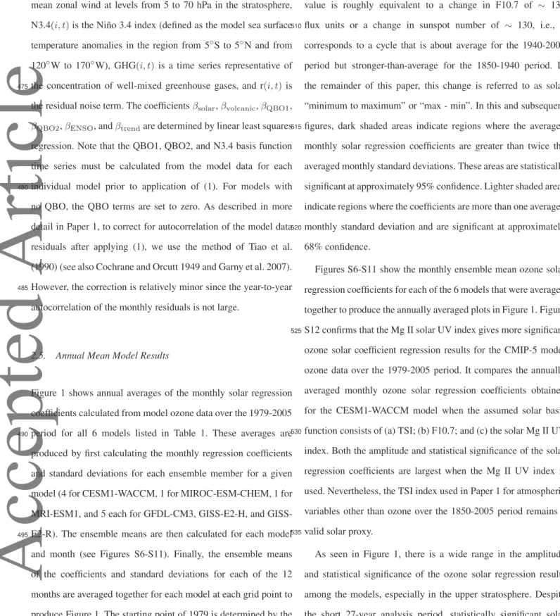
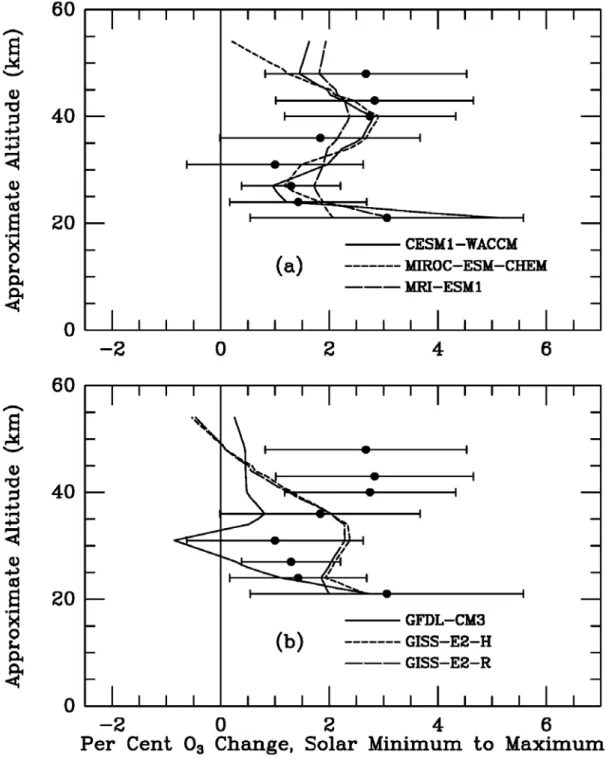
Figure 1 shows annual averages of the monthly solar regression coefficients calculated from model ozone data over the 1979-2005 period for all 6 models listed in Table 1. These averages are
490
produced by first calculating the monthly regression coefficients and standard deviations for each ensemble member for a given model (4 for CESM1-WACCM, 1 for MIROC-ESM-CHEM, 1 for MRI-ESM1, and 5 each for GFDL-CM3, GISS-E2-H, and GISS- E2-R). The ensemble means are then calculated for each model
495
and month (see Figures S6-S11). Finally, the ensemble means of the coefficients and standard deviations for each of the 12 months are averaged together for each model at each grid point to produce Figure 1. The starting point of 1979 is determined by the beginning of continuous satellite observations (section 3) while
500
the end point of 2005 is determined by the final year of the CMIP- 5 simulations. Ozone regression results are only shown at altitudes above 16 km since the vast majority of the ozone column is in the stratosphere. Results are not shown above 54 km since for 4 of the 6 models output is only provided to approximately this level.
505
Ozone solar regression coefficients are expressed as the per cent change in ozone concentration or mixing ratio for a change in the Mg II core-to-wing ratio of 0.0169. The latter value is roughly equivalent to a change in F10.7 of ∼ 130 flux units or a change in sunspot number of ∼ 130, i.e., it
510
corresponds to a cycle that is about average for the 1940-2000 period but stronger-than-average for the 1850-1940 period. In the remainder of this paper, this change is referred to as solar
“minimum to maximum” or “max - min”. In this and subsequent figures, dark shaded areas indicate regions where the averaged
515
monthly solar regression coefficients are greater than twice the averaged monthly standard deviations. These areas are statistically significant at approximately 95% confidence. Lighter shaded areas indicate regions where the coefficients are more than one averaged monthly standard deviation and are significant at approximately
520
68% confidence.
Figures S6-S11 show the monthly ensemble mean ozone solar regression coefficients for each of the 6 models that were averaged together to produce the annually averaged plots in Figure 1. Figure S12 confirms that the Mg II solar UV index gives more significant
525
ozone solar coefficient regression results for the CMIP-5 model ozone data over the 1979-2005 period. It compares the annually averaged monthly ozone solar regression coefficients obtained for the CESM1-WACCM model when the assumed solar basis function consists of (a) TSI; (b) F10.7; and (c) the solar Mg II UV
530
index. Both the amplitude and statistical significance of the solar regression coefficients are largest when the Mg II UV index is used. Nevertheless, the TSI index used in Paper 1 for atmospheric variables other than ozone over the 1850-2005 period remains a valid solar proxy.
535
As seen in Figure 1, there is a wide range in the amplitude and statistical significance of the ozone solar regression results among the models, especially in the upper stratosphere. Despite the short 27-year analysis period, statistically significant solar coefficients are obtained for 5 of the 6 models. Results for
540
models with little or no response in the upper stratosphere are shown in the lower panel (Figure 1 d, e, and f). Overall, the least significant coefficients were obtained for GFDL-CM3 while the most significant coefficients were obtained for MRI-ESM1.
The GFDL-CM3 results are not significant at the 2σ level with
545
Accepted Article
only marginally significant (1σ) values obtained in the lower stratosphere. The two GISS-E2 models produce a significant ozone response with maximum averaged amplitude of∼2% that is centered in the middle stratosphere near 10 hPa (∼32 km) while the response above 2 hPa is nearly zero.
550
The three models that do produce a significant averaged upper stratospheric response yield results shown in the top panel of Figure 1. The CESM1-WACCM response is centered at roughly 4 hPa (∼38 km) while the MIROC-ESM-CHEM and MRI-ESM1 responses are centered at a slightly higher level of 3 hPa or∼40
555
km. In all three cases, the peak amplitude averaged over all months is near 3%. Above the stratopause (∼1 hPa), the MRI-ESM1 response is largest (>2%) at high latitudes in both hemispheres.
As also seen in Figure 1, several models (CESM1-WACCM and GISS-E2-H) produce strong and apparently significant ozone
560
responses in the lower stratosphere (∼ 50 hPa). On the other hand, MIROC-ESM-CHEM and MRI-ESM1 produce reduced and much less significant responses at this level, indicating that the modeled lower stratospheric ozone response could be sensitive to details of the model formulation. In particular, because
565
the time period considered here includes two major volcanic eruptions (El Chich`on in 1982 and Pinatubo in 1991) that followed solar maxima in 1980 and 1989, it is possible that the lower stratospheric ozone signal in many of the models of Figure 1 is affected by aliasing, i.e., lack of complete orthogonality between
570
the solar and volcanic aerosol basis function time series (Solomon et al. 1996; Lee and Smith 2003). If so, then the magnitude of the apparent lower stratospheric 11-yr ozone response in many of the models of Figure 1 could be a function of how sensitive the simulated lower stratospheric chemistry and dynamics are to
575
volcanic aerosol effects (e.g., enhanced heterogeneous chemical ozone losses or radiative heating).
The extent to which aliasing between the solar and volcanic aerosol regression coefficients may occur in a version of WACCM (WACCM3.5) without a coupled ocean (forced using observed
580
SSTs and sea ice concentrations) has recently been investigated by Chiodo et al. (2014). By carrying out simulations over the 1960- 2004 period with and without including volcanic aerosol forcing, it was found that most of the apparent solar-induced variation of tropical lower stratospheric ozone and temperature in the model
585
is due to the two major volcanic events mentioned above. It was therefore inferred that the part of decadal variability in tropical lower stratospheric observations that can be attributed to solar variability may be smaller than previously believed. This may indeed be the case (see the next section).
590
However, the results of Figure 1 also suggest that any conclusions drawn from model simulations about the extent of volcanic aerosol aliasing in observations over the 1979-2005 period may depend on the model that is employed. To examine this possibility further, Figure S30 shows results of an MLR analysis
595
of the same model ozone data over the 1955-1981 period (prior to the El Chich`on eruption). The 11-yr ozone responses for all models are somewhat weaker at most altitudes than that shown in Figure 1, possibly because of a relatively weak solar cycle 20, which peaked near 1970. But the most dramatic reduction
600
in the response occurs in the lower stratosphere for 4 of the 6 models, CESM1-WACCM, GFDL-CM3, and the two GISS models. The remaining two models, MIROC-ESM-CHEM and MRI-ESM1, continue to show a lower stratospheric response that is proportionally of the same magnitude as obtained for the 1979-
605
2005 period (i.e., the ratio of the lower stratospheric response to the upper stratospheric response is nearly the same). From the combination of Figures 1 and S25, it can be inferred that the former four models produce an 11-yr lower stratospheric ozone response that is clearly affected by aliasing from the two volcanic
610
aerosol injection events while the responses for the latter two are not so strongly affected. Based only on this comparison of model results, however, it is difficult to evaluate which set of models is best able to simulate the lower stratospheric response, the former four or the latter two.
615
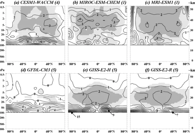
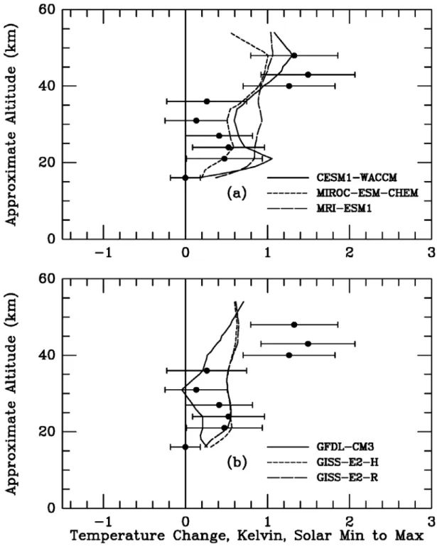
Figure 2 shows corresponding results for the annually averaged monthly temperature solar regression coefficients, expressed as the change in Kelvin from solar minimum to maximum (defined above). The individual ensemble mean monthly temperature solar regression coefficients are plotted in Figures S13-S18 for the 6
620
models. The annual mean results of Figure 2 are not very different from those shown in Paper 1, which used TSI rather than Mg II as the solar predictor and which analyzed the full suite of CMIP-5 models. Nevertheless, we show them here for completeness. As seen in the figure, the annual mean temperature results resemble
625
Accepted Article
the ozone results of Figure 1 since the ozone change contributes significantly to the radiative heating change from solar minimum to maximum in the stratosphere (e.g., Gray et al. 2009).
In the upper stratosphere, the three models in the top panel of Figure 2 produce the strongest responses, exceeding 1 K near the
630
stratopause. The GFDL-CM3 model produces the least significant results with amplitudes of∼0.5 K near the stratopause at most latitudes while the MRI-ESM1 model produces the strongest and most significant temperature response throughout the low-latitude stratosphere, exceeding 1 K above the 2 hPa level. The two
635
GISS-E2 models produce a significant temperature response of intermediate amplitude (>0.5 K) at most levels above∼30 hPa.
In the lower stratosphere at levels between 20 and 50 hPa, all models except GFDL-CM3 produce an apparently significant response of order 0.5 K or more from solar minimum to
640
maximum. However, as discussed above for ozone, it is likely that 11-yr signals in the lower stratosphere for many of these models are affected by aliasing from volcanic aerosol injections during the 1979-2005 period. To test this possibility, Figure S31 shows results of a similar analysis for the 1955-1981 period. The
645
apparently significant subtropical CESM1-WACCM responses at the 50 hPa level seen in Figure 2 are not present in Figure S31 and are replaced by a weakly significant equatorial response centered at about 20 hPa. The lower stratospheric responses for the MRI- ESM1 model and the two GISS-E2 models seen in Figure 2 are
650
no longer present in Figure S31. Only in the case of the MIROC- ESM-CHEM model does a weak lower stratospheric response remain in the 20-50 hPa tropical region. Thus, only MIROC-ESM- CHEM and possibly CESM1-WACCM could be simulating a true solar-induced tropical lower stratospheric temperature response.
655
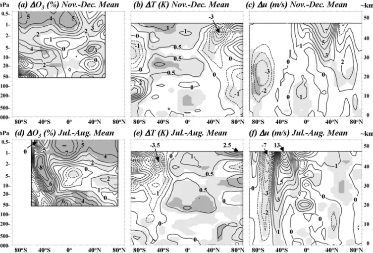
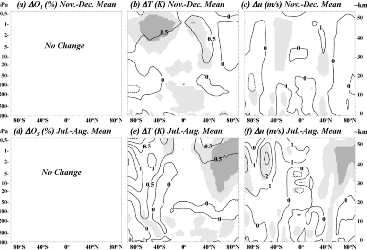
Turning to the monthly model ozone and temperature solar coefficients plotted in Figures S6-S11 and S13-S18, a seasonal evolution of the solar-induced signal is clearly present. In the summer hemisphere for all models, the thermal response in the upper stratosphere tends to shift toward higher latitudes, reflecting
660
the reduced solar-zenith angle during that season and the longer duration of daily solar heating at polar latitudes (midnight sun).
However, for the models in the top panels of Figures 1 and 2 with a relatively large upper stratospheric ozone and temperature
response (CESM1-WACCM, MIROC-ESM-CHEM, and MRI-
665
ESM1), there is also a tendency for large negative latitudinal ozone and temperature gradients to develop at high latitudes in the winter hemisphere. A similar tendency for temperature averaged over all high-top models during northern winter was also shown in Figure 7 of paper 1. Averaged over all 4 of the CESM1-WACCM
670
ensemble members, the large negative ozone and temperature gradients are mainly seen in the southern hemisphere in June and July but are also present in the northern hemisphere winter for 2 of the 4 members (not shown). In the case of the single MIROC- ESM-CHEM simulation, it occurs in December at high northern
675
latitudes and in July/August at high southern latitudes for both ozone and temperature. The same is true for the single MRI-ESM1 simulation. For the latter two models, the negative latitudinal gradients are noticeably larger in the southern hemisphere winter.
3. Comparisons With Observational Estimates
680
3.1. Ozone
Continuous global satellite remote sensing measurements of stratospheric ozone have been obtained since late 1978 (WMO 2007). These measurements, like those of SSI, are subject to uncertainties including degradation with time and intercalibration
685
offsets between different instruments. The longest continuous record of stratospheric ozone concentrations by a single instrument was obtained by the Stratospheric Aerosol and Gas Experiment (SAGE) II, beginning in November of 1984 and ending in August, 2005. The solar occultation measurement
690
technique employed by SAGE yields a relatively good vertical resolution approaching 1 km (e.g., McCormick et al. 1989).
Analyses of these data indicate substantial variations of 2 to 4%
from solar minimum to maximum extending from ∼ 5 hPa to and above the stratopause at low latitudes (e.g., Soukharev and
695
Hood 2006; Randel and Wu 2007; Kyr¨ol¨a et al. 2013; Remsberg 2014; see Figure 3c below). However, due to the sparse sampling of the SAGE solar occultation measurements, only annual mean regression coefficients can be accurately estimated.
A second long-term data set with more complete sampling
700
but less continuity and less vertical resolution (∼ 8 km) has been constructed at the U.S. Goddard Space Flight Center by
Accepted Article
merging together vertical ozone soundings by a series of SBUV instruments on Nimbus 7 (late 1978 to 1990) and subsequent U.S. National Oceanic and Atmospheric Administration (NOAA)
705
operational satellites (McPeters et al. 2013; Kramarova et al.
2013). The data obtained by the Nimbus 7 SBUV instrument were at a nearly constant local time while data acquired with SBUV/2 instruments on the NOAA satellites beginning with NOAA 11 in 1989 were more affected by orbital drifts that caused the local
710
time of measurement to vary during many of these missions. In the upper stratosphere (∼2 hPa and above), this can introduce artificial trends since there is a significant diurnal variation of ozone at these levels. Multiple linear regression (MLR) analyses of the merged SBUV data through 2003 yield a substantial annual
715
mean solar cycle variation of 3 to 4% at∼2 hPa and above in the upper stratosphere at low latitudes (Soukharev and Hood 2006;
Tourpali et al. 2007). As shown in the latter references, seasonal (e.g., northern winter and summer) mean regression coefficients can also be estimated using the more densely sampled, merged
720
SBUV data set. However, as discussed further below, the SBUV results have significant uncertainties imposed by the shortness of the data record (no more than 3.5 solar cycles) and the low vertical resolution of the individual profile measurements.
A third data set of interest is that obtained by the Halogen
725
Occultation Experiment (HALOE) on the Upper Atmosphere Research Satellite (UARS). Like SAGE, this experiment used the solar occultation technique but operated only from late 1991 to late 2005. HALOE retrieved ozone profiles on a pressure coordinate while SAGE ozone was retrieved on height levels,
730
which requires adoption of a long-term temperature record in order to convert the measurements to mixing ratios on pressure surfaces. Analyses of the HALOE ozone profile dataset yield somewhat reduced solar regression coefficients in the upper stratosphere compared to those estimated from the longer SAGE
735
and merged SBUV records (Soukharev and Hood 2006; Remsberg 2008). As discussed in the latter references, these reduced coefficients appear to agree better with model estimates near and above the stratopause than those derived from SAGE or SBUV.
However, it is unclear whether the reduced coefficients are a
740
consequence of the more direct HALOE retrieval technique or of the shorter record length (14 years).
To allow a more direct comparison with the annually averaged monthly model ozone solar regression coefficients of Figure 1 and the monthly coefficients of Figures S6-S11, the analysis
745
of Soukharev and Hood (2006) was extended to calculate monthly merged SBUV ozone regression coefficients using the same MLR model (1) that was applied to the CMIP-5 model data. Specifically, the monthly mean Version 8 merged SBUV ozone profile data set covering 1979-2003 was reanalyzed to
750
calculate individual monthly solar regression coefficients using the updated statistical model (1), including the more conservative autocorrelation correction described in section 2 and Paper 1. The ENSO basis function in this case is the observed Ni˜no 3.4 index and the two QBO empirical orthogonal functions are calculated
755
from the ERA Interim reanalysis data as described in Paper 1.
The N3.4 time series is lagged by 3 months to account for the observed delay in the stratospheric response to surface ENSO variability (e.g., Hood et al. 2010). The analysis is limited to the period prior to 2004 to allow direct comparisons with the results
760
of Soukharev and Hood (2006) and Tourpali et al. (2007) and to avoid any effects of a drift in the NOAA 16 orbit, which began in early 2004.
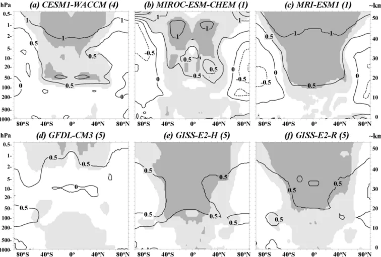
Figure 3a shows the annually averaged SBUV monthly solar regression coefficients to allow a direct comparison to the model
765
annually averaged coefficients of Figure 1. Specifically, Figure 3a was produced by averaging together the 12 monthly SBUV ozone solar regression coefficients and the corresponding standard deviations at each grid point. The individual monthly SBUV solar regression coefficients are plotted in Figure S19. Regression
770
coefficients and standard deviations at a given grid point were calculated from the 25 monthly means over 1979-2003. Figure 3b shows the annual mean SBUV solar regression coefficients obtained by considering each monthly anomaly (monthly mean minus long-term monthly mean) as an independent data point
775
(25 × 12 = 300). The annual mean coefficients of Figure 3b are more statistically significant than the annually averaged monthly coefficients of Figure 3a, as would be expected from the increased number of data points. In both cases, the per cent change in ozone from solar minimum to maximum is largest
780
in the uppermost stratosphere, especially in the tropics and at high latitudes in both hemispheres. In the tropical middle
Accepted Article
stratosphere (∼ 4 hPa), the response is a minimum and is statistically insignificant. Positive responses are also obtained in the extratropical middle stratosphere and in the lower stratosphere
785
near 50 hPa. The annually averaged monthly and annual mean ozone solar regression coefficients in Figures 3a,b are only marginally significant in the lower stratosphere. This differs from the results of Soukharev and Hood (2006) and Tourpali et al. (2007), who found apparently significant annual mean
790
coefficients in much of the lower stratosphere. The reduced significance obtained here is probably due to the use of alternate basis functions for volcanic aerosol and the QBO, as well as to the more conservative autocorrelation correction. However, the monthly regression coefficients remain statistically significant
795
during certain months, especially July and August as seen in Figure S19. Also, analyses of column ozone, which is dominated by lower stratospheric ozone, as a function of longitude and latitude yield significant solar regression coefficients at low latitudes during the northern summer and winter seasons (Hood
800
and Soukharev 2012).
Comparing the annually averaged monthly SBUV ozone solar regression coefficients of Figure 3a with the corresponding model coefficients of Figure 1, none of the models appears to yield an ozone response that agrees to first order with that derived from
805
the SBUV observations. None of the models produces a relative minimum in the tropical response near 4 hPa, although CESM1- WACCM produces a tropical minimum near the 20 hPa level.
The averaged monthly SBUV coefficients yield maxima near the stratopause exceeding 6% in the tropics, decreasing to∼4% at
810
middle latitudes, and increasing again to more than 6% at high latitudes. None of the models produces a response that maximizes near the tropical stratopause with reductions at midlatitudes. The 3 models in the top panel of Figure 1 do produce relatively large (>2%) ozone responses in the upper stratosphere but they are
815
centered near 4, 3, and 3 hPa, respectively, while the SBUV response is centered above 1 hPa. The 3 models in the bottom panel of Figure 1 produce responses at even lower levels (centered at or below the 10 hPa level).
However, some of the disagreements between Figure 3a and
820
Figure 1 may be a consequence of measurement uncertainties.
Although the merged SBUV data set is the only available record
with sufficient sampling and length to allow reasonable estimation of seasonally resolved ozone solar regression coefficients, there could be an artificial bias in these data toward higher altitudes.
825
Evidence that this may be the case comes from a consideration of the annual mean solar regression coefficients obtained from SAGE data, which have much better vertical resolution (∼1 km vs.∼8 km for SBUV). Figure 3c shows the result of an analysis of Version 6 SAGE II data (updated from Soukharev and Hood
830
2006) using the improved MLR model (1) and autocorrelation correction. In agreement with previous analyses (e.g., Randel and Wu 2007), the region of minimum tropical response based on SAGE data is centered near 10 hPa (∼31 km) while that of Figure 3b based on SBUV data is centered near 4 hPa (∼38 km). The
835
SAGE-derived ozone solar regression coefficients exceed 2% and are statistically significant at all levels above 5 hPa (∼36 km) continuing up to at least 0.5 hPa (∼54 km). On the other hand, the annual mean SBUV coefficients of Figure 3b exceed 2% in the tropics only at levels above 2 hPa (∼42 km).
840
Independent evidence that the ozone 11-yr solar regression coefficients derived from merged SBUV data are underestimated at levels below 2 hPa in the tropics has also been presented by Fioletov (2009). He predicted 11-yr ozone variations at low latitudes using the observed ozone response to short-term solar
845
rotational (∼ 27-day) UV variations and then compared these projected variations to observed decadal variations in data from the individual SBUV instruments. It was found (see his Figure 12) that the projected variation remained significant down to altitudes as low as 33 km even though no response was detectable
850
in the combined SBUV time series. Also, the SBUV data from the Nimbus 7 time period (1979-1990) contained an anomalously large 11-yr variation at altitudes above 44 km compared to the projected variation and to that recorded during later solar cycles.
Accepting the possibility that the actual observed ozone
855
response extends downward to at least the 5 hPa level in the tropics, the three modeled ozone responses in the top panel of Figure 1 compare more favorably with the observations. To illustrate this, Figure 4 plots tropical (25◦S to 25◦N) area- weighted averages of the SAGE II results from Figure 3c at a
860
series of pressure levels up to 1 hPa (∼ 48 km) together with corresponding averages of the model results of Figure 1. As
Accepted Article
seen in Figure 4a, the three models in the top panel of Figure 1 yield ozone response profiles that fall well within the 2σ error bars of the tropical mean SAGE II solar coefficients. As seen in
865
Figure 4b, the remaining models produce tropical mean upper stratospheric ozone responses that are outside of the 2σerror bars at altitudes above 40 km. Also, the altitude dependence of the solar ozone response for the latter models differs noticeably from that estimated from the SAGE II data.
870
3.2. Temperature
Continuous global satellite remote sensing measurements of atmospheric temperature also began in the late 1970’s. In Paper 1, model temperature solar responses were compared to estimates derived from the three most recent reanalysis meteorological
875
data sets, MERRA, ERA-Interim, and JRA-55 (Mitchell et al.
2014b). As discussed in Paper 1, a maximum solar-induced temperature response in the reanalyses of several Kelvin is obtained at low latitudes well above the stratopause (∼0.5 hPa), whereas the maximum expected theoretical response is about
880
half this amplitude and is centered near the stratopause (Gray et al. 2009). It was therefore suggested that increased errors in the reanalyses at levels above 1 hPa where data assimilation is poorly constrained by observations may be responsible for the unexpectedly large apparent solar signal. A comparison of
885
direct satellite Stratospheric Sounding Unit (SSU) measurements with reanalysis temperature time series supported this inference (Mitchell et al. 2014b).
Here, we consider specifically temperature and zonal wind data from one of the reanalyses, ERA Interim (Dee et al.
890
2011), which are publicly available to a level of 1 hPa (http://apps.ecmwf.int/datasets). As described in the Appendix (see also McLandress et al. 2014), at least one source of errors in this data set, step changes in upper stratospheric temperature occurring near the times of major changes in instrumentation or
895
processing of assimilated data, can be empirically minimized to produce an “adjusted” ERA Interim zonal mean temperature data set. Such an empirical minimization procedure is not generally applicable to other reanalyses (e.g., MERRA) because step changes were usually replaced with ramp functions in the archived
900
data sets.
Figure 5a shows the annually averaged monthly solar temperature regression coefficient derived from the adjusted ERA data over the 1979-2012 period, expressed as the change in Kelvin from solar minimum to maximum as defined in section 2.5. The
905
entire available 34-year record is considered rather than only the 1979-2005 period because the results change only slightly as compared to the shorter record and the statistical significance is improved. The individual monthly ERA Interim solar temperature regression coefficients are plotted in Figure S20. Figure 5b shows
910
the corresponding annual mean coefficient obtained when all available data points (12×34 = 408) are analyzed. The annual mean tropical upper stratospheric response is larger in peak amplitude (≥1.5 K) and is formally significant while the annually averaged monthly response of Figure 5a has a peak amplitude of
915
≥1 K and is only marginally significant. Overall, Figure 5b agrees well with previous studies, which analyzed the ERA-40 reanalysis data set through 2001 or extensions thereof (e.g., Crooks and Gray 2005; Frame and Gray 2010). It also agrees well with an alternate analysis of ERA Interim data by Mitchell et al. (2014b). As shown
920
in their Figure 7, the peak response in the tropics occurs near 2 hPa and the high-latitude maxima at 1 hPa in Figure 5b extend up to 0.3 hPa (∼55 km).
Comparing the annual ERA temperature results of Figure 5 with the annual observational ozone results of Figure 3, several
925
similarities are notable. First, in the tropics, the ozone response is largest in the upper stratosphere (down to∼2 hPa for SBUV and down to∼5 hPa for SAGE) while the temperature response is also largest in the tropical upper stratosphere (1 to 3 hPa).
Second, at high latitudes near the 1 hPa level, the temperature
930
response maxima of order 2 K compare favorably with the SBUV ozone response maxima of order 5-6%. A comparison of the monthly ERA temperature results of Figure S20 with the corresponding SBUV ozone results of Figure S19 shows that the high-latitude responses of both ozone and temperature occur
935
in the summer hemisphere. They are therefore presumably a consequence of the enhanced photolytic and radiative effects of more continuous solar radiation at reduced solar-zenith angles in the polar regions during the summer season. Third, the lower stratospheric subtropical temperature response maxima
940
agree qualitatively with responses seen in the SBUV data
c
Accepted Article
at comparable pressure levels, especially when the individual monthly responses are examined. Specifically, as seen in Figure 3a for the annually averaged SBUV monthly coefficients, marginally significant ozone response maxima of order 3% are present in the
945
subtropical lower stratosphere near 50 hPa. These coefficients are formally significant with larger amplitudes (up to 8%) during July and August (Figure S19). Similarly, the ERA Interim monthly coefficients are formally significant with amplitudes>0.5 K near 50 hPa only during June, July, and August (Figure S20).
950
Comparing the annual temperature responses of Figure 5 with the corresponding model responses of Figure 2, it is first apparent that the three models in the top panel of Figure 2 yield statistically significant minimum-to-maximum temperature changes in the tropical upper stratosphere that are closer in magnitude (>1 K) to
955
those obtained from the adjusted ERA data. This is further shown in Figure 6, which compares tropical averages of the ERA Interim temperature solar regression coefficients to similar averages of the model solar coefficients, analogous to the tropical ozone comparison in Figure 4. None of the models, however, produces
960
secondary temperature response maxima at high polar latitudes that are similar to those obtained in the ERA Interim data. The observationally estimated maxima are likely to be real because they are seen in both hemispheres in summer and correspond to similar polar ozone maxima found in SBUV data. An examination
965
of Figures S13-S18 shows that most of the models (except GFDL- CM3) produce broad maxima in the temperature response at high summer latitudes near the stratopause but the amplitudes are in the range of 1.0-1.5 K, which is less than obtained from the reanalysis data.
970
As discussed in section 2.5 in relation to Figures 2 and 6, many of the models produce broad positive responses in the tropical lower stratosphere that appear to be statistically significant but are probably influenced by aliasing from the effects of the El Chich`on and Pinatubo volcanic aerosol injection events (and
975
possibly ENSO events). In particular, CESM1-WACCM produces localized subtropical response maxima that are qualitatively similar to those obtained from the ERA Interim data. It is therefore entirely possible that some of the lower stratospheric thermal response in the ERA Interim results is also influenced by volcanic
980
aerosol and ENSO aliasing effects. However, the peak amplitudes
in the lower stratosphere for CESM1-WACCM (∼ 1 K) are nearly a factor of two larger than those in Figure 5b (∼ 0.6 K). Also, as seen in Figure S13, the monthly model temperature responses in this location are significant during most months
985
while, as seen in Figure S20, the corresponding observational monthly temperature responses near 50 hPa are significant only during NH summer. Similarly, as seen in Figure S6, the CESM1- WACCM 11-yr ozone response in the lower stratosphere is large and significant during nearly all months while, as seen in Figure
990
S19, the observationally estimated tropical ozone response near 50 hPa is significant only during NH summer. Hence, the aliasing effects in the observations could be less than is the case for CESM1-WACCM. Consistent with this possibility, at least one model, MIROC-ESM-CHEM, produces lower stratospheric 11-
995
yr ozone and temperature responses with amplitudes during the non-volcanic 1955-1981 period that are comparable to those during the volcanically-affected 1979-2005 period (Figures S30b and S31b). However, as already stated in section 2.5 above, without further information (e.g., investigation of the accuracies
1000
of different model sensitivities of lower stratospheric ozone and temperature to aerosol forcing), it is difficult to evaluate which model, CESM1-WACCM or MIROC-ESM-CHEM, is better able to simulate aliasing effects on observational solar regression coefficients in the lower stratosphere.
1005
3.3. Zonal Wind
The apparent offset errors found in ERA Interim temperature data in the upper stratosphere should be less problematic for the derived zonal wind field since the latter depends primarily on latitudinal temperature gradients, which are less sensitive to
1010
sudden steps in mean temperatures. The MLR model (1) was therefore applied to the ERA Interim zonal wind data over 1979- 2012 to obtain the monthly solar regression coefficients plotted in Figure S21. Again, we consider the extended time period because the results are very similar to those obtained for 1979-2005 and
1015
the statistical significance is slightly increased. The regression coefficients are expressed as the change in the zonal wind in meters/second from solar minimum to maximum, as defined in section 2.5.