An electrokinetic LB based model for ion transport and macromolecular electrophoresis

An electrokinetic LB based model for ion transport and macromolecular electrophoresis

Raffael Pecoroni Supervisor: Michael Kuron

July 8, 2016

1 Introduction & Motivation

So far an mesoscopic coarse-grained model for DNA transport through nanopores has been discussed. But we have taken no account of the solvent in that the DNA has been suspended. Additionally the solvent usually contain charged solutes due to dissociation of molecules at boundary surfaces or simply by autoprotolysis of water.

Thus we will have a closer look on electrolytes and its behaviour in motion. We will derive the underlying equations and furthermore solve them.

2 Electrokinetic Equations

The dynamics of charged solutes in a fluid is described by the electrokinetic equations which form a coupled nonlinear system of differential equations. One must take into account

• hydrodynamics of the solvent,

• the solute dynamics and

• electrostatics (ionic solutes or charged boundaries).

In the following this equation system is derived.

2.1 Hydrodynamics

We assume an incompressible fluid, so the velocity field is free of divergence which gives us the restriction

∇ · ~ u = 0 . (1)

The dynamics of the solvent is specified by the Navier-Stokes-Equation (NSE) which provides momentum conser- vation and takes then the following form [4]

ρ ∂

∂t ~ u + ρ~ u · ∇~ u = η∇ ² ~ u − ∇p + f ~ ext . (2)

ρ(~ r) is here the density of the solvent, ~ u(~ r) the velocity field at each point, η the dynamic viscosity, p the hydrostatic

pressure, and f ~ _ext is the external force. In our case moving solutes interact with the fluid and therefore cause a

momentum transfer. So this external force term couples the solvent to the solute behaviour. Both equations

describe hydrodynamics entirely so we can dedicate ourselves to the solute dynamics.

2.2 Dynamics of solute species

Conservation of mass is stated by the continuity conservation law with the density of species ρ _k (~ r, t)

∂

∂t ρ k + ∇~j k = 0 . (3)

Each species k has to be treated on its own if there are more than one solute species suspended in a fluid.

Two different phenomena contribute to the transport flux of species in a solvent: diffusion and advection (~j k =

~j _k ^diff + ~j _k ^adv ). We will consider them separately deriving the equations and eventually merge them.

2.2.1 Diffusion

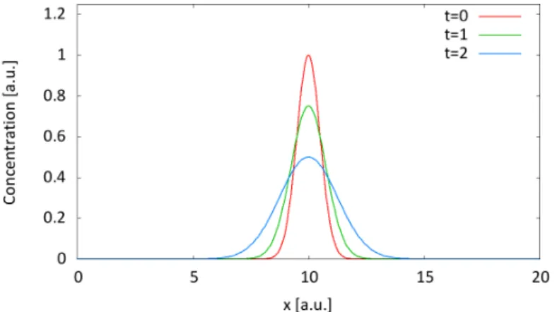
A varying concentration of the solute in a solvent leads to a flux from regions of higher concentration towards regions lower concentration like depicted in figure 1.

Figure 1: Diffusive behaviour of a gaussian distributed concentration plotting different points in time. The maximum decreases as the concentration distribution broadens. The integral under the curve keeps constant that implies mass conservation.

The diffusive term is determined by Fick’s law [3, 4]

~j _k ^diff = −D k ∇ρ k (4)

with the diffusion coefficient D _k that describes how fast the solute spreads. If the species are charged or an electric field E = −∇φ exists, Fick’s law is extended by a term depending on the ratio of electric potential and thermal energy

~j ^diff _k = −D k ∇ρ k − D k z k e k B T ρ k ∇φ

| {z }

due to electric field

(5)

with the valency z _k of the k-th species.

2.3 Advection

Solute species are also moving due to the fluid flow ~ u that has to be obtained from NSE. This phenomena is called advection and is displayed in figure 2. In contrast to diffusion the concentration moves here in space but does not broaden. The flux is defined by

~j _k ^adv = ~ uρ _k . (6)

Inserting both diffusive flux and advective flux into equation (3) we result in Poisson-Nernst-Planck Equation (PNP) that is the fundamental equation of the solute behaviour.

∂

∂t ρ k = −∇(~j _k ^diff + ~j _k ^adv )

= ∇

D k ∇ − ~ uρ k + D k z k e k B T ρ k ∇φ

. (7)

Figure 2: Advective behaviour of a gaussian distributed concentration. Due to the fluid velocity ~ u the concen- tration moves in space [5]

This equation is essential for electrokinetic phenomena like electrophoresis or electro-osmotic flow. The coupling between PNP equation (7) and NSE (2) is obviously involved by the velocity field ~ u in PNP and f ~ ext in NSE. But the electrostatic potential needs to be considered still.

2.4 Electrostatics

The electrostatic potential φ that is necessary to solve the PNP is obtained by Poisson’s equation. We assume that the dielectric permittivity is constant and end up with

∇ ² φ = − ρ(~ r)

= −4πλ B k B T ρ k (8)

with the Bjerrum length λ B = _4πk ^e

B

T indicating at which distance between two charged particles the electrostatic potential is comparable to the thermal energy. This Poisson equation couples to PNP through ρ k . [4]

So far the hydrodynamic NSE describing the solvent, the PNP equation that represents the motion of ions and the electrostatic Poisson equation has been derived. Together ((1),(2),(7),(8)) they form the full set of electrokinetic equations that has to be solved.

3 Numerical scheme for solving electrokinetic equations

This Equation system is nonlinear and has several coupling terms. Analytic solutions can be found only in very simple geometries or in specific cases like stationarity. For time evolution and processes that are far from equilibrium the electrokinetic equations has to be solved numerically.

For hydrodynamics there already exist an powerful method.

3.1 Lattice Boltzmann method (LBM)

The most intuitive way is to discretize Navier-Stokes Equation. But solving it is complicated because it is not local and therefore hardly can parallelized.

On mesoscopic length scales the Lattice Boltzmann method is the most suitable way for simulation. It is based on Boltzmann equation

∂

∂t f(~ r, ~ v, t) + ∇f (~ r, ~ v, t) = C(f (~ r, ~ v, t), t) (9) with the probability distribution function f (~ r, ~ v, t) that describes the probability of how many particles with velocity

~

v are located at place ~ r. On the right hand side the collision operator describes the behaviour of interacting particles.

Assuming an exponential relaxation towards equilibrium we can rewrite the collisional term with the so called BGK

approximation _τ ¹ (f ^eq −f ) with the equilibrium distribution function f ^eq and the specific time scale of the relaxation

τ .

Discretizing the Boltzmann equation in time and space a lattice is introduced (figure 3) with the base vectors

~ c i connecting the nodes. In the figure the common D3Q19 lattice is used standing for 3-dimensional and 19 connectivity links.

Figure 3: Lattice that is introduced in order to discretize Boltzmann equation. {~ c i } are the connection links between neighbouring nodes [8]

We result finally in the LB equation

f _i (~ r + ~ c _i dt, t + dt) − f _i (~ r, t) = 1

τ (f _i ^eq (~ r, t) − f _i (~ r, t)) . (10) This scheme is easy to implement and suitable for parallel computation. Moreover it is momentum and mass conserving and in the continuity limit it corresponds to NSE. The right hand side of (10) is called collison step that performs the interaction of particles at each node. Afterwards the streaming step on the left hand side is performed that shifts the distribution function after collision to the next node. Then again the collision step is executed and so on. [7, 1]

Thus we are able to solve the fluid dynamics of the solvent with the conventional LB method.

3.2 Discretizing Diffusion and Advection

In 1997 Warren proposed a technique to numerically solve the solute dynamics. He used the underlying grid of Lattice Boltzmann for hydrodynamics and discretized the PNP equation the same way. Capuani in 2004 improved this technique. Instead of considering the solute population on the lattice cells he computed the fluxes between two neighbouring cells.

3.2.1 Diffusion

In order to discretize the diffusive flux we assume ~ u = 0. The continuity equation (3) yields after integrating it over the volume V 0 of a cell

∂

∂t Z

V

ρ _k dV = − I

A

~j _k ^diff · ~ n dA (11)

with the normal surface vector ~ n. Discretizing this equation end up in V 0 ρ k (~ r, t + 1) − V 0 ρ k (~ r, t) = −A 0

X

i

~j _ki ^diff (~ r) (12)

with the flux ~j ki of species k in direction ~ c i . A 0 is here not the surface of the cell but it contains information about the connectivity between two neighbouring cells and is therefore defined by the geometry of the lattice.

But still the fluxes need to be discretized. This is achieved by the following form

~j _ki ^diff = D _k (ρ _k (~ r) − ρ _k (~ r + ~ c _i )) − D _k z _k e A 0 k B T

ρ _k (~ r) + ρ _k (~ r + ~ c _i )

2 (φ(~ r) − φ(~ r + ~ c _i )) . (13) In particular the discretization expression of the flux has to be chosen carefully. Capuani et al. [1] used a different expression that was computationally more expensive and suffered off artifacts in special cases.

Considering the fluxes provides automatically mass conservation down to machine accuracy. Moreover boundary

conditions can be implemented simply because the flux into the boundary vanishes (~j ki = 0). [1, 4]

3.2.2 Advection

It is possible to discretize the advective flux the same way. The fluid velocity ~ u is interpolated onto the links.

Basically discretization accompany with errors, thus arising artifacts in simulation.

Capuani used a different ansatz. The flow velocity ~ u(~ r) in a cell is determined at first. Then this cell is virtually displaced by ~ r → ~ r + ~ udt resulting in an overlap of the virtual cell with the neighbouring cells. The fraction of the overlap and the cell volume is computed. Finally the solutes flowing into that cell are assigned according to the ratio. (figure 4).

Figure 4: Method for calculating the discrete advection flux. Virtual displacement of the origin cell ~ r → ~ r +~ udt leads to an overlap of the virtual cell with the neighbouring cells. The fraction of this overlap over the cell volume yields the amount of solutes moving into that cell.

3.3 Electrostatics

So far hydrodynamics and solute dynamics have been treated. For solving the electrostatic Poisson equation a successive over-relaxation scheme (SOR) is applied. We therefore have to discretize space. The 3-dimensional laplacian operator has to be discretized too. For sake of convenience this is depicted here for a 1-dimensional laplacian.

∇ ² φ = ∂ ²

∂x ² φ(x) = 1

h ² [φ(x − 1) − 2φ(x) + φ(x + 1)] (14)

Now the Poisson equation rewrites to a linear system of equations Aφ(~ x) = ρ(~ x) with the matrix A that is populated with the coefficients of equation (14) and ~ x the vector that counts off the grid nodes.

Finally A has to be inverted in order to compute the electrostatic potential. Gaussian algorithm is the simplest method for inverting but it scales unfavourable with O(N ³ ) and does not obligatory converge. Hence SOR is applied which is an iterative scheme. It incorporates the solution from the step before and also an additional parameter that has to be adapted for an considerable increase of convergence. [4, 1]

3.4 Spurious fluxes

As mentioned above one has to take care when the diffusive is discretized. Furthermore the discrete advection scheme suffers of artifacts if the fluid motion is interpolated onto the links. These artifacts are called spurious fluxes. They arise due to discretization errors and may lead to unphysical behaviour of the system, for instance a finite solute flow along a boundary in equilibrium.

We can get rid of these spurious fluxes if the grid resolution is increased. However, computation time increases rapidly. Beyond the choice of an appropriate diffusive and advective flux, G. Rempfer additionally reduced the spurious fluxes by a modified external force. Both improvements reduce the flux by several orders of magnitude.

[6, 1]

4 Electrophoresis

Until now we have dealt with the derivation and discretization of the electrokinetic equation. Electrophoresis is a

phenomena that can be simulated with the presented numerical scheme.

Figure 5: A negatively charged colloid at rest with surface charge σ and radius R is located in an electrolyte with two species. Counterions are attracted and form a electrical double layer (EDL). Within the EDL the electric potential decays exponentially, the Debye length λ D is assigned to the decay. [10]

Electrophoresis describes the motion of a charged colloid in a solvent under the influence of an electric field. The colloid is simulated as boundary condition. The surrounding of the colloid contains counterions getting attracted by the colloid forming a cloud around it whereas co-ions are repelled like depicted in figure 5. The counterion cloud mostly screens the surface charge within the so called electrical double layer (EDL). Latter decreases exponentially within the Debye length λ D .

An applied electric field on the one hand directly exerts an electrostatic force onto the colloid while a viscous force is decelerating it on the other hand (figure 6) since the counterions move to the opposite side dragging water that retards the colloid.

Figure 6: Positively charged colloid with a distorted EDL in an electric field. The accelerating force is due to electrostatics, the friction force originates from the counterion motion to the opposite direction [9]

In steady-state and for weak electric field the colloid velocity ~ v is proportional to an applied electric field ~ v = µ ~ E with mobility µ as proportional constant. O’Brien and White derived an analytical expression for the mobility [5]

assuming low salt concentration c _s and sufficiently low surface charges. In this regime they discovered a maximum in mobility that arises if c _s is large enough.

With LB based model it is possible to simulate this electrophoretic phenomena and compare it to the theoretical

predictions of O’Brien and White. In figure 7 the reduced mobility is plotted over the reduced ζ-potential indicating

the surface charge of the colloid. For low c _s and in the linear regime the simulation result fits exactly to the

theory. At the nonlinear regime ζ > ˜ 4 deviations increase. A maximum mobility is found here in contrary to the

predictions of O’Brien and White underlying the restrictions of the analytic solution. High salt concentration results

in a deviation even in linear regime. In this restricted range of validity (low c s and low ζ-potential) the simulation

coincide with the analytical solution of O’Brien and White. [5] This shows that the derived LB based method

Figure 7: Reduced Mobility of the colloid is plotted over the reduced ζ-potential that is proportional to the surface charge of the colloid. Comparison of simulation (filled symbols) to theoretical predictions of O’Brien and White (empty symbols) for an electrolyte with high (blue) and low (red) salt concen- tration. It coincides for the case of low salt concentration and low ζ-potentials [2]

reproduces theory and is a useful method if electrolytes within complex geometries are simulated.

5 Conclusion

Within this handout we have discussed the electrokinetic equations and a powerful discretization method that is able to simulate a wide range of electrolytes, that can be composed of multiple ionic solutes. There already exist several methods reducing spurious fluxes which are a result of discretization errors. Moreover we benchmarked this method by reproducing electrophoresis.

References

[1] F. Capuani, I. Pagonabarraga, and D. Frenkel. Discrete solution of the electrokinetic equations. Journal of Chemical Physics, 121(2):973–986, 2004.

[2] G. Giupponi and I. Pagonabarraga. Colloid electrophoresis for strong and weak ion diffusivity. Physical Review Letters, 106(24):2–5, 2011.

[3] B. J. Kirby. Micro- and Nanoscale Fluid Mechanics: Transport in Microfluidic Devices. Cambridge University Press, 2010.

[4] M. Kuron. Efficient Lattice Boltzmann Algorithms for Colloids Undergoing Electrophoresis. Master thesis, Stuttgart, 2015.

[5] R. W. O’Brien and L. R. White. Electrophoretic mobility of a spherical colloidal particle. Journal of the Chemical Society, Faraday Transactions 2: Molecular and Chemical Physics, 74(0):1607–1626, 1978.

[6] G. Rempfer, G. B. Davies, C. Holm, and J. de Graaf. Limiting Spurious Flow in Simulations of Electrokinetic Phenomena. arxiv:1604.02054, apr 2016.

[7] U. D. Schiller. Thermal fluctuations and boundary conditions in the lattice Boltzmann method. Dissertation, Johannes Gutenberg-University Mainz, 2008.

[8] A. Schneider, D. Conrad, and M. B¨ ohle. Lattice Boltzmann Simulation of the Flow Field in Pump Intakes—A New Approach. Journal of Fluids Engineering, 137(3).

[9] Wikipedia:. Electrophoresis. online, retrieved 2016-06-23.

[10] Wikipedia:. Zeta Potential. online, retrieved 2016-06-20.